3902 wileyonlinelibrary.comjournalmec Molecular Ecology.docx

3902 | wileyonlinelibrary.com/journal/mec Molecular
Ecology. 2019;28:3902–3914.© 2019 John Wiley & Sons Ltd
1 | I N T R O D U C T I O N
Maynard‐Smith and Haig (1974) recognized the influence of
selection
on linked neutral sites, proposing that strong positive selection
could
reduce genetic diversity at nearby sites. This process is now
referred
to as a ‘selective sweep’. Much later, Charlesworth, Morgan,
and
Charlesworth (1993) proposed that deleterious mutations could
also
affect genetic diversity at nearby sites, because some haplotypes
would be removed from the population as selection acts against
linked deleterious alleles. They named this process background
se‐
lection (BGS). Both selective sweeps and background selection
af‐
fect genetic diversity; they both reduce the effective population
size
and distort the site frequency spectrum (SFS) of linked loci.
Empirical
evidence of a positive correlation between genetic diversity and
recombination rate has been reported in several species (Cutter
&
Payseur, 2013), including Drosophila melanogaster (Begun &
Aquadro,
1992; Elyashiv et al., 2016), humans (Spencer et al., 2006),

collared
flycatchers, hooded crows and Darwin's finches (Dutoit et al.,
2017;
see also Vijay et al., 2017).
BGS is also expected to affect FST (Charlesworth, Nordborg, &
Charlesworth, 1997; Cruickshank & Hahn, 2014; Cutter &
Payseur,
2013; Hoban et al., 2016). The negative relationship between
effec‐
tive population size Ne and FST is captured in Wright's
classical in‐
finite island result; FST =
1
1+4Ne(m+�)
(Wright, 1943), where m is the
migration rate and µ is the mutation rate. One might therefore
ex‐
pect that loci under stronger BGS would show higher FST.
Many authors have also argued that, because BGS reduces the
within‐population diversity, it should lead to high FST
(Cruickshank
Received: 20 May 2018 | Revised: 19 June 2019 |
Accepted: 3 July 2019
DOI: 10.1111/mec.15197
O R I G I N A L A R T I C L E
Background selection and FST: Consequences for detecting
local adaptation

Remi Matthey‐Doret | Michael C. Whitlock
Department of Zoology and Biodiversity
Research Centre, University of British
Columbia, Vancouver, BC, Canada
Correspondence
Remi Matthey‐Doret, Department of
Zoology and Biodiversity Research Centre,
University of British Columbia, Vancouver,
BC V6T 1Z4, Canada.
Email: [email protected]
Funding information
The work was funded by NSERC
Discovery Grant RGPIN‐2016‐03779 to
MCW and by the Swiss National Science
Foundation via the fellowship Doc.Mobility
P1SKP3_168393 to RMD.
Abstract
Background selection is a process whereby recurrent deleterious
mutations cause a
decrease in the effective population size and genetic diversity at
linked loci. Several
authors have suggested that variation in the intensity of
background selection could
cause variation in FST across the genome, which could
confound signals of local ad‐
aptation in genome scans. We performed realistic simulations of
DNA sequences,
using recombination maps from humans and sticklebacks, to
investigate how varia‐
tion in the intensity of background selection affects FST and
other statistics of popu‐
lation differentiation in sexual, outcrossing species. We show

that, in populations
connected by gene flow, Weir and Cockerham's (1984;
Evolution, 38, 1358) estimator
of FST is largely insensitive to locus‐to‐locus variation in the
intensity of background
selection. Unlike FST, however, dXY is negatively correlated
with background selec‐
tion. Moreover, background selection does not greatly affect the
false‐positive rate
in FST outlier studies in populations connected by gene flow.
Overall, our study in‐
dicates that background selection will not greatly interfere with
finding the variants
responsible for local adaptation.
K E Y W O R D S
adaptation, evolutionary theory, local adaptation, population
genetics—theoretical,
population structure
mailto:
https://orcid.org/0000-0001-5614-5629
https://orcid.org/0000-0002-0782-1843
mailto:[email protected]
| 3903MATTHEY‐DORET AnD WHITLOCK
& Hahn, 2014; Cutter & Payseur, 2013; Hoban et al., 2016).
Expressed in terms of heterozygosities, FST =
HT−HS
HT
=1−

HS
HT
, where
HT is the expected heterozygosity in the entire population and
HS
is the average expected heterozygosity within subpopulations
(HS
and HT are also sometimes called πS and πT, e.g. Charlesworth,
1998). All else being equal, a decrease in HS would indeed lead
to
an increase in FST. However, all else is not equal; HT is also
affected
by BGS (Charlesworth et al., 1997). Therefore, in order to
under‐
stand the effects of BGS on FST, we must understand the
relative
impact of BGS on both HS and HT. (This paragraph has
expressed
FST by one definition that mirrors Nei's GST, but Weir and
Cockerham's (1984) θ estimates a similar quantity, FST =
�D
�S+�D
,
where �D =
d−1
d
(

�T −�S
)
and d is the number of populations sam‐
pled. For the majority of this paper, we consider this more
broadly
used measure from Weir and Cockerham.) By either measure of
FST, if HS and HT are changed in the same proportion by BGS,
there
would be no effect on FST.
Charlesworth et al. (1997) as well as Zeng and Corcoran (2015)
have performed more sophisticated analysis measuring the
effect
of BGS on FST through numerical simulations. Charlesworth et
al.
(1997) reported that BGS reduces the within‐population hetero‐
zygosity HS slightly more than it reduces the total
heterozygosity
HT, causing a net increase in FST. The effect on FST reported
is quite
substantial, but, importantly, their simulations were not meant
to be
realistic. The authors highlighted their goal in the methods:
The simulations were intended to show the quali‐
tative effects of the various forces studied […], so
we did not choose biologically plausible values […].
Rather, we used values that would produce clear‐cut
effects.
For example, talking about their choice for the deleterious
muta‐
tion rate of 8 × 10−4 per site:
This unrealistically high value was used in order for

background selection to produce large effects [...]
Much of the literature on the effect of BGS on FST is based
on the results in Charlesworth et al. (1997), even though they
only intended to provide a proof of concept (see also Zeng &
Charlesworth, 2011 and Zeng & Corcoran, 2015). They did not
at‐
tempt to estimate how strong of an effect BGS has on FST in
real
genomes.
The intensity of BGS varies throughout the genome as a conse‐
quence of variation in recombination rate, selection pressures
and
mutation rates. Therefore, if BGS significantly affects FST, we
should
expect that baseline FST to vary throughout the genome. It is
im‐
portant to distinguish two separate questions when discussing
the
effect of BGS on FST: (a) How does BGS affect the average
genome‐
wide FST? and (b) How does locus‐to‐locus variation in the
intensity
of BGS affect locus‐to‐locus variation in FST? The second
question is
of particular interest to those trying to identify loci under
positive
selection (local selection or selective sweep). Locus‐to‐locus
varia‐
tion in FST due to BGS potentially could be confounded with
the FST
peaks created by positive selection. In this paper, we focus on
this
second question.

The identification of loci involved in local adaptation is often
performed via FST outlier tests (Hoban et al., 2016; Lotterhos
&
Whitlock, 2014). Other tests exist to identify highly divergent
loci
such as cross‐population extended haplotype homozygosity (XP‐
EHH; Sabeti et al., 2007), comparative haplotype identity
(Lange
& Pool, 2016) and cross‐population composite likelihood ratio
(XP‐
CLR; Chen, Patterson, & Reich, 2010). FST outlier tests, such
as fdist2
(Beaumont & Nichols, 1996), bayescan (Foll & Gaggiotti, 2008)
or flk
(Bonhomme et al., 2010), look for genomic regions showing
par‐
ticularly high FST values to find candidates for local
adaptation. If
BGS can affect FST unevenly across the genome, then regions
with
a high intensity of BGS could potentially have high FST values
that
could be confounded with the pattern caused by local selection
(Charlesworth et al., 1997; Cruickshank & Hahn, 2014). BGS
could
therefore inflate the false‐positive rate when trying to detect
loci
under local selection.
The potential confounding effect of BGS on signals of local ad‐
aptation has led to an intense effort trying to find solutions to
this
problem (Aeschbacher, Selby, Willis, & Coop, 2017; Bank,
Ewing,
Ferrer‐Admettla, Foll, & Jensen, 2014; Huber, Degiorgio,

Hellmann,
& Nielsen, 2016). Many authors have understood from
Cruickshank
and Hahn (2014) that dXY should be used instead FST in outlier
tests
(e.g. McGee, Neches, & Seehausen, 2015; Yeaman, 2015;
Whitlock
& Lotterhos, 2015; Brousseau et al., 2016; Picq, Mcmillan, &
Puebla,
2016; Payseur & Rieseberg, 2016; Hoban et al., 2016; Vijay et
al.,
2017; see also Nachman & Payseur, 2012). FST is a measure of
pop‐
ulation divergence relative to the total genetic diversity, while
dXY is
an absolute measure of population divergence defined as the
prob‐
ability of nonidentity by descent of two alleles drawn in the two
different populations averaged over all loci (Nei, 1987; Nei,
1987
originally called it DXY but, here, we follow Cruickshank &
Hahn's,
2014 terminology by calling it dXY ). The argument is that
because
FST is a measure of divergence relative to the genetic diversity
and
dXY an absolute measure of divergence and because BGS
reduces
genetic diversity (Cruickshank & Hahn, 2014; Hoban et al.,
2016),
then BGS must affect FST but not dXY, a claim that we will
investigate
in this paper.
Whether BGS can affect genome‐wide FST under some con‐
ditions is not in doubt (Charlesworth et al., 1997), but whether

locus‐to‐locus variation in the intensity of BGS present in
natural
populations substantially affects variation in FST throughout
the
genome is very much unknown. Empirically speaking, it has
been
very difficult to measure how much of the genome‐wide varia‐
tion in genetic diversity is caused by BGS, as opposed to
selective
sweeps or variation in mutation rates (Cutter & Payseur, 2013;
see also attempts in humans by Cai, Macpherson, Sella, &
Petrov,
2009, McVicker, Gordon, Davis, & Green, 2009 and Elyashiv et
al., 2016). We are therefore in need of realistic simulations that
3904 | MATTHEY‐DORET AnD WHITLOCK
can give us more insight into how BGS affects genetic diversity
among populations and how it affects the statistics of
population
divergence.
In this article, we investigate the effect of BGS in structured
pop‐
ulations with realistic numerical simulations. Our two main
goals are
(a) to quantify the impact of locus‐to‐locus variation in the
intensity
of BGS on FST (Weir & Cockerham, 1984) and dXY (Nei,
1987) and
(b) to determine whether BGS inflates the false‐positive rate of
FST
outlier tests.

2 | M E T H O D S
Our goal is to perform biologically plausible simulations of the
local
genomic effects of background selection in biological settings
with
ongoing gene flow among populations. BGS is expected to vary
with
strength of selection (itself affected by gene density), mutation
rate
and recombination rate across the genome. We used data from
real
genomes to simulate realistic covariation in recombination rates
and
gene densities. We chose to base our simulated genomes on two
eu‐
karyote recombination maps derived from sticklebacks and
humans,
because these two species have attracted a lot of attention in
stud‐
ies of local. The recombination rate variation in humans is
extremely
fine scale, but it presents the potential issue that it is estimated
from
linkage disequilibrium data. As selection causes linkage
disequilib‐
rium to increase, estimates of recombination rate at regions
under
strong selection may be under‐estimated, which might bias the
simu‐
lated variance in the intensity of BGS. Although the
recombination
map for stickleback is much less fine‐scaled, the estimates are
less
likely to be biased as they are computed from pedigrees.

Our simulations are forward in time and were performed using
the simulation platform simbit version 3.69. We simulated
nonover‐
lapping generations with hermaphroditic, diploid individuals
and
random mating within patches. Selection occurred before
disper‐
sal. The code and user manual are available at https
://github.com/
RemiM atthe yDore t/SimBit. The rational for using a new
simulation
platform is because all existing simulation platforms today were
too
slow for our needs (See Appendix S1). To double check our
results,
we also ran some simulations with slim (Haller & Messer, 2017)
and
nemo (Guillaume & Rougemont, 2006) (see Appendix S1),
confirming
that we obtain consistent distributions of genetic diversity and
of FST
among simulations. For simulations with slim and nemo,
independent
simulations were parallelized with gnu parallel (Tange, 2011).
2.1 | Genetics
For each simulation, we randomly sampled a sequence of about
10 cM from either the stickleback (Gasterosteus aculeatus)
genome
or the human genome (see Treatments below) and used this
genomic
location to determine the recombination map and exon locations
for a simulation replicate. For the stickleback genome, we used
the
gene map and recombination map from Roesti, Moser, and

Berner
(2013). Ensembl‐retrieved gene annotations were obtained from
Marius Roesti. For the human genome, we used the
recombination
map from The International HapMap Consortium (2007) and the
gene positions from NCBI and positions of regulatory sequences
on
Ensembl (Zerbino et al., 2018). We excluded sex chromosomes
to
avoid complications with haploid parts of the genomes. As
estimates
of mutation rate variation throughout the genome are very
limited,
we assumed that the haploid mutation rate varies from site to
site
following an exponential distribution with mean of 2.5 × 10−8
per
generation (mean estimate from Nachman & Crowell, 2000).
More specifically, we first randomly sampled a sequence of 105
nucleotides, which we will refer to as the focal region. All of
the sta‐
tistics (defined under the section Statistics below) are
calculated
only on this focal region of each simulation. Nucleotides that
occur
in locations determined to be exons in the sampled genomic map
are
subject to selection (see Selection), while all other nucleotides
are
assumed to be neutral. The focal region itself contained on
average
~0.44 genes for the human genome and ~3.15 genes for the
stick‐
leback genome.

We simulated a 5 cM region on each side of the focal region
(re‐
sulting in a window of 10 cM plus the map distance covered by
the
specific focal region of 105 sites) in order to capture the local
effects
of background selection. In these 10 cM flanking regions, we
only
tracked exons (or in the case of the human genetic map, exons
and
regulatory sequences). In the nearest 1 cM on each side of the
focal
region, as well as within the focal region, we individually
simulated
each nucleotide as a bi‐allelic locus. On the remaining outer 4
cM, to
improve the speed and RAM usage of the process, we tracked
the
number of mutations in blocks of up to 100 nucleotides. For
these
blocks, we tracked only the number of mutations but not their
loca‐
tion within the block. Ignoring recombination within a block
likely
had little effect on the results because the average
recombination
distance between the first and last site of a block is of the order
of
10−6 cM. The expected number of segregating sites within a
block is
4N�
∑2N−1
i=1

�
1
i
�
, which for a mutation rate per block of 10−6 and a
population size of N = 10,000 is ~0.42. The probabilities of
having
more than one mutation and more than two mutations (based on
a
Poisson approximation) are therefore only approximately 6.7%
and
0.9%, respectively. Overall, the level of approximation used is
very
reasonable.
2.2 | Selection
As we are interested in the effect of BGS, we modelled the
effects
of purifying selection against novel deleterious mutations. Each
nucleotide in the exons (and regulatory sequences for the human
genetic map) is subject to purifying selection with a selection
coef‐
ficient against mutant alleles determined by a gamma
distribution
described below. For focal regions that include exons, statistics
are
computed over a sequence that is at least partially under direct
pu‐
rifying selection.

To create variance in selection pressures throughout the ge‐
nome, each exon (and regulatory sequence for the human
genetic
https://github.com/RemiMattheyDoret/SimBit
https://github.com/RemiMattheyDoret/SimBit
map) has its own gamma distribution of heterozygous selection
co‐
efficients s. The mean and variance of these gamma
distributions
are drawn from a bivariate uniform distribution with correlation
coefficient of 0.5 (so that when the mean is high, so is the vari‐
ance) bounded between 10−8 and 0.2 for both the mean and the
variance. These bounds were inspired by the methodology used
in
Gilbert et al. (2017). The gamma distributions are bounded to
one.
Figure S1 shows the overall distribution of selection coefficient
s, with 2% of mutations being lethal and an average deleterious
selection coefficient for the nonlethal mutations of 0.074. In the
treatment Low selection pressure (see Treatments below), the
upper
bounds for the mean and variance of the gamma distributions
were set to 0.1 instead of 0.2. To improve the performance of
our
simulations, we assumed multiplicative fitness interactions
among
alleles, where the fitness of heterozygotes at locus i is 1 − si
and
the fitness of the double mutant is (1 − si)

2. Any mutation changes
the state of the locus to the other possible allele.
As a consequence of our parameter choices, our genome‐wide
deleterious mutation rate was about 1.6 in sticklebacks and
about 3
in humans. 9.8% of the stickleback genome and 2.7% of the
human
genome were under purifying selection. For comparison, the ge‐
nome‐wide deleterious mutation rate is estimated at 2.2 in
humans
(Keightley, 2012) and 0.44 in rodents (Keightley & Gaffney,
2003).
To our knowledge, there is currently no such estimation for
stick‐
lebacks. Note, however, that the above estimates cannot reliably
detect mutations that are quasi‐neutral (s « 1/(2N)). By our
distri‐
bution of selection coefficients, 49% of all deleterious
mutations
have a heterozygote selection coefficient lower than 1/(2Ne)
when
Ne = 1,000 (42% when Ne = 10,000). The fraction of selection
coeffi‐
cients that are of intermediate effect (between 1/(2Ne) and
10/(2Ne))
is 10% when Ne = 1,000 (7% when Ne = 10,000).
It is worth noting that, in rodents, about half of the deleteri‐
ous mutations occur in noncoding sequences (Keightley &
Gaffney,
2003). Our simulations using human genetic map had all exons
and
all regulatory sequences under purifying selection. With our
simu‐
lations based on the stickleback genome, however, only exons

were
under purifying selection. It is therefore possible that we would
have
over‐estimated the deleterious mutation rate in gene‐rich
regions
and under‐estimated the deleterious mutation rate in other
regions,
especially in stickleback. This would artificially increase the
locus‐
to‐locus variation in the intensity of BGS in our simulations,
which is
conservative to our conclusions.
2.3 | Demography
In all simulations (except for those matching the Charlesworth
et al.
(1997) results), we started with a burn‐in phase with a single
popula‐
tion of N diploid individuals, lasting 5 × 2N generations. The
popula‐
tion was then split into two populations of N individuals each
with
a migration rate between them equal to m. After the burn‐in
phase,
each simulation was run for 5 × 2N more generations for a total
of
10 × 2N generations.
2.4 | Treatments
We explored the presence and absence of deleterious muta‐
tions over two patch sizes, three migration rates, two genomes
and three selection scenarios. We considered a default design
and explored variations from this design. The Default design
had a population size per patch of N = 1,000, a migration rate of

m = 0.005 and used the stickleback genome for its
recombination
map and gene positions. As deviations from this default design,
we explored modification of every variable, one variable at a
time.
The Large N treatment has N = 10,000. The Human Genetic
Map
treatment uses the human genome for gene positions, regulatory
sequences and recombination map. The treatments No Migration
and High Migration have migration rates of m = 0 and m = 0.05,
respectively. The Constant µ treatment assumes that all sites
have
a mutation rate of 2.5 × 10−8 per generation. The Low selection
pressure treatment simulates lower selection coefficients (see
sec‐
tion Selection above).
To test the robustness of our results and because it may be rel‐
evant for inversions, we also performed simulations where the
re‐
combination rate for the entire 10 cM region was set to zero. As
a
check against previous work, we qualitatively replicated the
results
of Charlesworth et al. (1997) by performing simulations with
similar
assumptions as they used. We named this treatment CNC97. In
our
CNC97 simulations, N = 2,000, m = 0.001 and 1,000 loci were
all
equally spaced at 0.1 cM apart from each other with constant
selec‐
tion pressure with heterozygotes having fitness of 0.98 and
mutant
homozygote fitness of 0.9 and constant mutation rate μ =
0.0004.

Note that Charlesworth et al. (1997) used partially recessive
alleles
which we mimic for this case, but the simulations for the other
cases
considered in this paper use multiplicative interactions between
al‐
leles. We performed further checks against previous works that
are
presented in Appendix S1. A full list of all treatments can be
found
in Table 1.
In all treatments (except Large N), we performed 4,000 simula‐
tions: 2,000 simulations with BGS and 2,000 simulations
without se‐
lection (where all mutations were neutral). For Large N,
simulations
took more memory and more CPU time. For the Large N case,
we
performed 1,000 simulations with background selection and
1,000
simulations without selection.
We set the generation 0 at the time of the split. The state of
each population was recorded at the end of the burn‐in period
(gen‐
eration −1) and at generations 0.001 × 2N, 0.05 × 2N, 0.158 ×
2N,
1.581 × 2N and 5 × 2N after the split. For N = 1,000, the
sampled
generations are therefore −1, 2, 100, 316, 3,162 and 10,000.
2.5 | Predicted intensity of background selection
In order to investigate the locus‐to‐locus correlation between
the

predicted intensity of BGS and various statistics, we computed
B, a
statistic that approximates the expected ratio of the coalescent
time
with background selection over the coalescent time without
background selection
(
B=
TBGS
Tneutral
)
. B quantifies how strong BGS is ex‐
pected to be for a given simulation (Nordborg, Charlesworth, &
Charlesworth, 1996). Furthermore, B has been used to predict
the
effect of BGS on FST (Zeng & Corcoran, 2015). A B value of
0.8 means
that BGS has caused a drop of neutral genetic diversity of 20%
com‐
pared to a theoretical absence of BGS. Lower B values indicate
stronger BGS.
Both Hudson and Kaplan (1995) and Nordborg et al. (1996)
have
derived the following theoretical expectation for B.

where ri is the recombination rate between the focal site and the
ith
site under selection, and si is the heterozygous selection
coefficient
at that site, and ui is the (haploid) mutation rate at the ith site.
By this
formula, B is bounded between 0 and 1, where 1 means no BGS
at all
and low values of B mean strong BGS. We computed B for all
sites in
the focal region and report the average B for the region. While
B is cal‐
culated just for the focal region, it is based on the effects of all
selected
sites in the simulated region of just over 10 cM.
For the stickleback genome, B values ranged from 0.03 to
0.99 with a mean of 0.84 (Figure S2). For the human genome, B
values ranged from 0.20 to 1.0 with a mean at 0.91. In the No
Recombination treatment, B values range from 10−10 to 0.71
with
a mean of 0.07.
Excluding the treatments No Recombination and CNC97, we ob‐
served that simulations with BGS have a genetic diversity
(whether
HT or HS; HT data not shown) 6%–25% lower than simulations
without BGS. Messer and Petrov (2013) simulated a panmictic
population, looking at a sequence of similar length inspired
from a
gene‐rich region of the human genome, and reported a similar
de‐
crease in genetic diversity. Under the No Recombination
treatment,
this average reduction of genetic diversity due to BGS is 53%.

In
empirical studies, linked selection is estimated to reduce genetic
diversity by up to 6% according to Cai et al. (2009) or 19%–
26%
according to McVicker et al. (2009) in humans. In D.
melanogaster,
where gene density is higher, the reduction in genetic diversity
due to linked selection is estimated at 36% when using Kim and
Stephan (2000)'s methodology and is estimated at 71%
reduction
using a composite likelihood approach (Elyashiv et al., 2016).
In
mice, BGS alone cannot explain fully the reduction in genetic
di‐
versity at low recombination sites, and selective sweeps due to
positive selection are responsible for the majority of the
reduction
in diversity due to linked selection (Booker & Keightley, 2018).
It
is worth noting that, because we were interested in the locus‐to‐
locus variation of various statistics in response to varying
intensity
of BGS, we did not simulate a whole genome worth of BGS, and
hence, the overall reduction in genetic diversity that we observe
should not be understood as a genome‐wide effect of BGS.
2.6 | FST outlier tests
In order to know the effect of BGS on outlier tests of local
adapta‐
tion, we used a variant of fdist2 (Beaumont & Nichols, 1996).
We
chose fdist2 because it is a simple and fast method for which
the
assumptions of the test match well to most of the demographic
sce‐

narios simulated here (although it is a poor match to the No
migra‐
tion scenario, which has not reached equilibrium in our
simulation
conditions). Because the program fdist2 is not available through
B=exp
(
−
∑
i
uisi
(si +ri)
2
)
Treatment N m Genome Other BGS
Default 1,000 0.005 Stickleback – Yes
No
High migration 1,000 0.05 Stickleback – Yes
No
Large N 10,000 0.005 Stickleback – Yes
No

Human genetic
map
1,000 0.005 Human – Yes
No
Low selection
pressure
1,000 0.005 Stickleback Low selection
pressure
Yes
No
Constant µ 1,000 0.005 Stickleback Constant mutation
rate
Yes
No
No migration 1,000 0 Stickleback – Yes
No
No recombination 1,000 0.005 Stickleback Absence of
crossover
Yes
No
CNC97 2,000 0.001 NA See Methods

section
Yes
No
T A B L E 1 Summary of treatments. For
all treatments but CNC97, the average
mutation rate was set to 2.5 × 10−8
per site, per generation and the mean
heterozygous selection coefficient as
described in the text
the command line, we rewrote the fdist2 algorithm in r and c++.
Source code can be found at https ://github.com/RemiM atthe
yDore
t/Fdist2.
Our fdist2 procedure is as follows: first, we estimated the
migra‐
tion rate from the average FST of the specific set of simulations
consid‐
ered (m= 1−FST
4
(
d
d−1
)2

NFST
; Charlesworth, 1998) and then running 50,000
simulations each lasting for 50 times the half‐life to reach
equilibrium
FST given the estimated migration rate (Whitlock, 1992). For
each SNP,
we then selected the subset of fdist2 simulations for which
allelic di‐
versity was <0.02 away from the allelic diversity of the SNP of
interest.
The p‐value is computed as the fraction of fdist2 simulations
within
this subset having a higher FST than the one we observed. The
false‐
positive rate is then defined as the fraction of neutral SNPs for
which
the p‐value is lower than a given α value, using α = 0.05. We
confirmed
that the results were similar for other α values.
For the outlier tests, to avoid issues of pseudo‐replication, we
considered only a single SNP (randomly sampled from the focal
re‐
gion) per simulation whose minor allele frequency is >0.05.
Then,
we randomly assembled SNPs from a given treatment into
groups of
500 SNPs to create the data file for fdist2. We have 4,000
simula‐
tions (2,000 with BGS and 2,000 without BGS) per treatment
(Large
N is an exception with only 2,000 simulations total), which
allowed

eight independent false‐positive rate estimates per treatment
(four
estimates with BGS and four without BGS). In each treatment,
we
tested for different false‐positive rate with and without BGS
with
both a Welch's t test and a Wilcoxon test.
2.7 | Statistics
FST and dXY are both measures of population divergence. In
the litera‐
ture, there are several definitions of FST, and we also found
potential
misunderstanding about how dXY is computed.
There are two main estimators of FST in the literature: GST
(Nei,
1973) and θ (Weir & Cockerham, 1984). In this article, we
focus on θ
as an estimator of FST (Weir & Cockerham, 1984). There are
also two
methods of averaging FST over several loci. The first method is
to sim‐
ply take an arithmetic mean over all loci. The second method
consists
at calculating the sum of the numerator of θ over all loci and
dividing it
by the sum of the denominator of θ over all loci. Weir and
Cockerham
(1984) showed that this second averaging approach has lower
bias
than the simple arithmetic mean. We will refer to the first
method as
the ‘average of ratios’ and to the second method as ‘ratio of the
aver‐

ages’ (Reynolds, Weir, & Cockerham, 1983; Weir &
Cockerham, 1984).
In this article, we use FST as calculated by ‘ratio of the
averages’, as
advised by Weir and Cockerham (1984). To illustrate the effects
of
BGS on the biased estimator of FST, we also computed FST as a
simple
arithmetic mean (‘average of the ratio’), and we will designate
this sta‐
tistic with a subscript FST (average of ratios).
dXY is a measure of genetic divergence between two
populations
X and Y. Nei (1987) defined dXY as,
where L is the total number of sites, Al is the number of alleles
at the lth
site, and xl,k and yl,k are the frequency of the kth allele at the
lth locus in
the population X and Y, respectively.
Some population genetics software packages (e.g. egglib; De
Mita & Siol, 2012) average dXY over polymorphic sites only,
instead
of averaging over all sites, as in Nei's (1987) original definition
of
dXY. This measure averaged over polymorphic sites only will
be
called dXY‐SNP; otherwise, we use the original definition of
dXY by
Nei (1987).
We report the average FST, dXY and within‐population genetic
diversity HS =

∑L
l=1
�
1−
∑Al
k=1
x2
l,k
�
∕L. Our main results lie in the com‐
parison between simulations with BGS and simulations without
BGS within each treatment. Because theoretical expectations
exist for the strength of BGS on genetic diversity within
popula‐
tions, we also investigated the relationships between this
theoret‐
ical expectation, B and FST, FST (average of ratios), dXY,
dXY‐SNP, and HS in
five independent tests for each treatment and at each generation.
For this, we used Pearson correlation test, Spearman rank
correla‐
tion tests, ordinary least squares regressions, robust regressions
(using M‐estimators; Huber, 1964) and permutation tests. The
re‐
sults were systematically consistent. Permutations tests of
Pearson's correlation coefficients were performed with 50,000
iterations. Because all tests were congruent, we only report the
Pearson correlation coefficient and the p‐values from
permutation

tests.
The data presented below are available on Dryad (https ://doi.
org/10.5061/dryad.44vr58d).
3 | R E S U LT S
The distributions of FST values from simulations with BGS are
extremely similar to the distribution of FST values of
simulations
where all mutations were neutral. This remains true even in the
most extreme treatment with no recombination. This general
dXY =
∑L
l=1
�
1−
∑Al
k=1
xl,kyl,k
�
L
F I G U R E 1 Violin plots showing the distribution of FST
values
for the Default treatment (labelled ‘With Recombination’) and
for
the No Recombination treatment. Simulations with BGS are

shown
in red, and simulations without BGS are in blue. The means and
standard errors are displayed with dots and error bars (although
the error bars are barely visible because the standard errors are
so
small)
https://github.com/RemiMattheyDoret/Fdist2
https://github.com/RemiMattheyDoret/Fdist2
https://doi.org/10.5061/dryad.44vr58d
result is exemplified in Figure 1 by comparing the Default treat‐
ment to the No Recombination treatment. As we have a large
number of simulations, the means of the distributions of FST
are significantly different between simulations with BGS and
simulations without BGS for both the Default (Wilcoxon tests:
W = 47,875,000; p = .00002) and the No Recombination
(Wilcoxon
tests: W = 47,804,000; p = .002) treatments, but the increase in
mean FST due to BGS is only 4.3% for the Default treatment
and
2.6% in the No Recombination treatment.
Figure 2 shows the means and standard errors for FST, dXY and
HS
for all treatments. For most treatments, FST is very little
changed by
BGS, even when HS and dXY are strongly affected.
Figure 3 shows the correlation between the predicted B and
the statistics FST, dXY and HS for Default at the last
generation. FST is

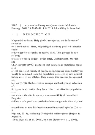
not correlated with B (p = .24, r = −.02). The strongest
correlations
with B are observed for the statistics dXY (p = 4 × 10
−5, r = .06) and
HS (p = 4 × 10
−5, r = .06). In fact, the two statistics dXY and HS are
very highly correlated (p < 2.2 × 10−16, r = .99). This high
correlation
F I G U R E 2 Comparisons of mean FST (left column), dXY
(central column) and HS (right column) between simulations
with (black) and
without (grey) BGS. Error bars are 95% CI derived from
permutations. Significance of difference between mean FST
with and without BGS
based on permutation tests is indicated with stars (***p < .001;
**p < .01; *p < .05)
F I G U R E 3 Correlation between B and FST, HS and dXY
for the last generation (5 × 2N generations after the split) of the
Default treatment.
Each grey dot is a single simulation where there is BGS. The
large black dot is the mean of the simulations with no BGS. The
p‐values are
computed from a permutation test, and r is the Pearson's
correlation coefficient. p‐values and r are computed on both
simulations with and
without BGS. Results are congruent when computing the
correlation coefficients and p‐value on the subset of simulations
that have BGS
Low
BGS

High
BGS
r : .02
P : .24
0
0.05
0.1
0.15
0.0 0.5 1.0
B
F
S
T
Low
BGS
High
BGS
r : .06
P : 4 x 10 5
0.0000
0.0005
0.0010

0.0015
0.0 0.5 1.0
B
d
X
Y
Low
BGS
High
BGS
r : .06
P : 4 x 10 5
0.0000
0.0005
0.0010
0.0015
0.0 0.5 1.0
B
H
S

explains the resemblance between the central and right graphs
of
Figure 3. All correlations between the statistics HS, FST, FST
(aver‐
age of ratios), dXY, and dXY‐SNP and B are summarized in
Tables S1–S5,
respectively.
When looking at correlations between B and the statistics of
population divergence, the No Migration treatment is an
exception to
the other treatments. For the No Migration treatment, FST is not
sig‐
nificantly correlated with B at early generations but become
slightly
correlated as divergence rises to an FST of 0.6 and higher. dXY
shows
an opposite pattern. dXY is very significantly correlated with B
at early
generations and seemingly independent of B at the last
generation.
Note that for FST all correlation coefficients are always very
small.
The largest r2 observed for FST is r
2 = 0.01 (found for FST No Migration).
As expected, in the CNC97 simulations, there is a strong differ‐
ence between simulations with BGS and simulations without
BGS
for all three statistics (FST, dXY and HS) at all generations
(Welch's t
tests; all p < 2.2 × 10−16; Figure 2).

FST averaged over loci as advised by Weir and Cockerham
(1984)
was generally less sensitive to BGS than FST calculated as an
average
of ratios (compare Tables S2 and S3). This effect is again
partially
visible in the correlations with B. Figure S2 illustrates the
sensitivity
of FST (average of ratios) in the worst case, the No
Recombination treat‐
ment. This sensitivity is driven largely by rare alleles and goes
away
when minor alleles below a frequency of 0.05 are excluded.
The observed false‐positive rate (FPR) for the FST outlier test
is relatively close to the α values except for No Migration (with
and
without BGS) and CNC97 (with BGS). Excluding the
intentionally
unrealistic treatment CNC97, we do not see more significant
dif‐
ferences between the FPR with and without BGS than we would
expect by chance (Figure 4). There are other statistics of inter‐
est that one can consider to investigate whether BGS causes
FST
outliers. Among all treatments (excluding CNC97), the fraction
of
SNPs that are associated with a FST that is >10 times the
average
FST in its particular treatment is 0.075% with BGS and 0.085%
without BGS. These numbers go up to 1.7% and 1.8% for SNPs
that have a FST five times greater than the average FST, for
treat‐
ments with BGS and without BGS, respectively. We have also
computed, in each treatment, the ratio of the largest FST to the
average FST. Among treatments without BGS, the largest FST

was
on average 12.2 times the average FST, while among treatments
with BGS, the largest FST was on average 12.1 times the
average
FST. With an α threshold of 0.001, we observe that 0.080% and
0.083% of the SNPs turn out false positives among treatments
without BGS and among treatment with BGS, respectively. For
the conditions considered in this paper, BGS does not signifi‐
cantly increase the rate of FST outliers.
4 | D I S C U S S I O N
In agreement with previous works (e.g. Charlesworth, 2012;
Elyashiv et al., 2016; Messer & Petrov, 2013; Nordborg et al.,
1996; Vijay et al., 2017; Zeng & Charlesworth, 2011), we show
that background selection reduces genetic diversity, both within
and among populations. The magnitude of this effect is very
simi‐
lar to previous realistic simulations (Messer & Petrov, 2013).
The
effect of BGS on FST is however rather small and does not
seem
F I G U R E 4 Comparison of false‐positive rate (FPR)
returned by
fdist2 between simulations with BGS (black) and without BGS
(grey)
for all treatments by generation. The significance level is 0.05
and is
represented by the horizontal dashed line. Significance based on
a
Welch's t test is indicated with stars (***p < .001; **p < .01; *p
< .05).
With Wilcoxon tests, none of the treatments displayed here
comes

out as significant
to impact the overall distribution of FST in the sexual
outcrossing
conditions that we study here (Figure 1). The relative
robustness
of FST to variation in the intensity of BGS is contrary to what
has
been found in less realistic simulations (Charlesworth et al.,
1997;
Zeng & Corcoran, 2015).
FST was also generally not significantly correlated with B. The
only exception is for the No Migration treatment, where, after
many
generations, as the average FST becomes very high (FST > 0.5),
we
observe a slight, yet significant, negative correlation between
the
expected effects of BGS, B and FST (intense BGS lead to high
values
of FST). This highlights that FST is not completely insensitive
to BGS,
but FST is largely robust to BGS in cases of reasonable levels
of gene
flow among populations. The observed correlation coefficients
are
always very small with not a single r2 value >1%. It is
important to
highlight that B has not been defined in order to estimate the
effect
of BGS onto FST but only for the effect of BGS on HS in a

panmictic
population, although Zeng and Corcoran (2015) predict that B
can be
used to determine the effects of BGS on FST.
In this study, we investigated the locus‐to‐locus variation
in the intensity of BGS and how it affects FST. Future research
is needed to attempt a theoretical estimate of the genome‐wide
effect of BGS on FST (but see Charlesworth et al., 1997; Zeng
&
Corcoran, 2015). Our work has been restricted to the
stickleback
and human recombination maps. While these two genomes are
reasonable representatives of many eukaryotic genomes, they
are not good representatives of more compact genomes such as
bacterial genomes or yeasts. Our simulations used randomly
mat‐
ing diploid populations. Nonrandom mating, selfing and asexual
reproduction could also affect our general conclusion and
poten‐
tially strongly increase the effects of BGS on FST
(Charlesworth
et al., 1997). Also, we did not explore the effect of haploid
selec‐
tion as we only considered autosomes (see Charlesworth, 2012).
We have explored two population sizes, but we could not
explore
population sizes of the order of a million individuals (like D.
melan‐
ogaster) and still realistically simulate such long stretches of
DNA.
It is not impossible that a much greater population size or a
more
complex demography could result in BGS having a greater
effect
on FST than what we observed here (Torres, Szpiech, &

Hernandez,
2018). In the No Recombination treatment, we have explored
cases
of complete suppression of recombination over stretches of
DNA
of, on average, 0.8% of the stickleback genome and our results
were still consistent. However, we have not explored the effect
of suppression of recombination over greater regions, such as a
whole chromosome that does not recombine. We have also not
explored such suppression of recombination in perfectly
isolated
populations as we mainly focused on interconnected popula‐
tions. It is not impossible that in such cases we might observe a
greater impact of BGS on FST such as those observed in Zeng
and
Corcoran (2015) and reproduced in Appendix S1.
Some have argued that, because BGS reduces the within‐popula‐
tion diversity, it should lead to high FST (Cruickshank & Hahn,
2014;
Cutter & Payseur, 2013; Hoban et al., 2016). All else being
equal, this
statement is correct. However, BGS reduces HT almost as much
as HS
(Figure S4). It is therefore insufficient to consider only one
compo‐
nent, and we must consider the ratio of these two quantities cap‐
tured by the definition of FST, FST =
(�T−�S)
�T+
�
S

d−1
. This ratio, as we have
shown, appears to be relatively robust to BGS. While
genome‐wide
BGS might eventually be strong enough to affect FST values, it
ap‐
pears that locus‐to‐locus variation in the intensity of BGS is not
strong enough to have much impact on FST in outcrossing
sexual or‐
ganisms, at least as long as populations are not too highly
diverged.
We also investigated the consequences of BGS on the widely
used but imperfect estimator, FST (average of ratios), for which
FST mea‐
sures for each locus are averaged to create a genomic average.
It is
well known that FST (average of ratios) is a biased way to
average FST over
several loci (Weir & Cockerham, 1984); however, its usage is
rela‐
tively common today. In our simulations, FST (average of
ratios) is more af‐
fected by BGS than FST. Interestingly, FST (average of ratios)
is most often
higher with weaker BGS. The directionality of this correlation
may
seem unintuitive at first. To understand this discrepancy,
remember
that BGS affects the site frequency spectrum; we observed that
BGS
leads to an excess of loci with low HT (results not shown, but
see
Charlesworth, Charlesworth, & Morgan, 1995; see also contrary

ex‐
pectation in Stephan, 2010). Loci associated with very low HT
also
have low FST (Figure S3), a well‐known result described by
Beaumont
and Nichols (1996). As BGS creates an excess of loci with low
HT and
loci with low HT tend to have low FST, BGS can actually
reduce FST
(average of ratios). After filtering out SNPs with a minor allele
frequency
lower than 5%, most of the correlation between FST (average of
ratios) and
B is eliminated (Figure S2).
The absolute measure of divergence dXY is more sensitive to
BGS
than FST (Figure 2; Tables S2 and S4). Regions of stronger
BGS are
associated with low dXY. This is in agreement with correlation
tests
between B and dXY. The effect, although significant, is of
relatively
small size. BGS should affect dXY by its effect on the expected
het‐
erozygosity, and this effect should be greater early in
divergence and
with migration, compared to divergence occurring because of
new
mutations in isolated populations. This is consistent with the
results
of our simulations. This result is in agreement with Vijay et al.
(2017)
who reported a strong correlation between HS and dXY when
FST is
low (FST ≈ 0.02), but this correlation breaks down when

studying
more distantly related populations (FST ≈ 0.3).
As BGS also leads to a reduction of the number of polymor‐
phic sites, BGS has an even stronger effect on dXY‐SNP than
on dXY
(Figure S2). (The measure that we call dXY‐SNP is dXY
improperly calcu‐
lated based only on polymorphic sites, as is done in some
software
packages.)
Zeng and Corcoran (2015) approximated the effect of back‐
ground selection on FST accounting for the effect that BGS has
on
the effective population size (FST =
1
4NBm+1
). With our simulations,
we report only little to no association between this expectation
and the actual FST (see Figure S5). We think that BGS is a
complex
process and reducing its effect on FST by its theoretical
expecta‐
tion of the statistic B is misleading. Below, we discuss some of
the
reasons.
Because most deleterious mutations are recessive (García‐

Dorado et al., 2000; Peters, Halligan, Whitlock, & Keightley,
2003;
Shaw & Chang, 2006), the offspring of migrants, who enjoy an
in‐
creased heterozygosity compared to local individuals, will be at
a se‐
lective advantage. The presence of deleterious mutations
therefore
leads to an increase in the effective migration rate (Ingvarsson
&
Whitlock, 2000), which leads to a decrease in FST. In our
simulations
however, mutational allelic effects are close to additive, and
hence,
we should not expect to see much effect of BGS on the effective
mi‐
gration rate. Additionally, patches that have a lower average
fitness
will receive migrants that are comparably fitter and hence will
enjoy
a higher effective migration rate than other patches. This should
also
lead to decrease FST.
There is one additional factor that may weaken the connection
between the FST predicted based on Ne = NB used in the Zeng
and
Corcoran approximation. This approximation implicitly assumes
that
the effects of new deleterious alleles on the effective population
size are immediate. However, in a structured population
connected
by migration (and when migration is strong relative to the
strength of
selection), alleles will typically migrate before selection acts to
elim‐

inate them. As a result, BGS affects the global genetic variation
and
the local genetic variation in a similar way. In other words, if
alleles
migrate before the effects of selection on linked loci is fully
realized,
then BGS will affect coalescent times of alleles between
populations
in a parallel way to how it affects coalescent times of alleles in
the
same population, resulting in a weakened effect on FST
compared
to that predicted by the Zeng and Corcoran approximation. We
an‐
ticipate that much stronger selection coupled with weaker
migra‐
tion would show a larger effect on FST, as is in fact the case in
the
parameters chosen by Zeng and Corcoran in their simulations
(see
Appendix S1).
Another reason why one might not observe a correlation be‐
tween intensity of BGS and FST throughout the genome is
because
mutation rate is auto‐correlated throughout the genome; neutral
sequences closely linked to sequences that frequently receive
dele‐
terious mutation are also likely to experience frequent neutral
muta‐
tions. As a high mutation rate leads to low FST values (FST ≅
1
1+4Ne(m+�)
,

Wright, 1943), autocorrelation in mutation rate may also act as
to
reduce the effect of BGS on FST. This effect is however likely
to be
negligible as long as m » µ.
Recently, evidence of a correlation between recombination rate
and FST has been interpreted as likely being caused by
deleterious
mutations rather than positive selection, whether the divergence
between populations is very high (e.g. Cruickshank & Hahn,
2014),
moderately high (Vijay et al., 2017) or moderately low (Torres
et al.,
2018). Here we showed the BGS is unlikely to explain all of
these
correlations between FST and recombination rate, especially in
cases
with relatively low divergence among populations. As positive
se‐
lection has been shown to also have an important effect on ge‐
netic diversity (Eyre‐Walker & Keightley, 2009; Hernandez,
Kelley,
Elyashiv, Melton, & Auton, 2011; Macpherson, Sella, Davis, &
Petrov,
2007; Sattath, Elyashiv, Kolodny, Rinott, & Sella, 2011;
Wildman,
Uddin, Liu, Grossman, & Goodman, 2003), it would be
important to
investigate whether positive selection (selective sweeps and
local
adaptation) could be an important driver of the correlations
between
FST and recombination rate. More research would be needed to

in‐
vestigate whether this is true.
McVicker et al. (2009) attempted an estimation of B values in
the human genome (see also Elyashiv et al., 2016). They did so
using
equations from Nordborg et al. (1996). As there is little
knowledge
about the strength of selection throughout the genome, to our
un‐
derstanding, this estimation of B values should be highly
influenced
by the effects of beneficial mutations as well as deleterious
muta‐
tions. Torres et al. (2018) reused this data set and found a slight
asso‐
ciation between B and FST among human lineages. It is
plausible that
this correlation between B and FST could be driven by positive
selec‐
tion rather than by deleterious mutations; this possibility should
be
further explored.
Our fdist2 analysis shows that the false‐positive rate does not
differ in simulations with BGS or without BGS (Figure 4). The
only
exceptions concern the unrealistic CNC97 treatment. The
average
FST at the last generation of the No Migration treatment is
>0.8.
With such high FST, the FST outlier method, fdist2, does not
seem
to perform well and both the simulations without BGS and with
BGS lead to very high false‐positive rates (0.472 without BGS
and

0.467 with BGS; Figure 4). Beaumont and Nichols (1996)
showed
that the fdist2 procedure is problematic for nonequilibrium pop‐
ulations, especially when FST is >0.5 (see section
nonequilibrium
populations from their results), especially when the number of
subpopulations sampled is low. It therefore sounds plausible
that
fdist2 would poorly apply to our No Migration treatment. While
other issues may intervene in FST outlier methods (Lotterhos &
Whitlock, 2014), our results show that BGS should not
represent
any significant issue for outcrossing sexual species with moder‐
ately low mean FST.
We have shown that BGS affects HS and dXY but has only a
very minor effect on FST among sexual outcrossing populations
connected by gene flow. Many authors (Cutter & Payseur, 2013;
Hoban et al., 2016) have raised concerns that BGS can strongly
reduce our ability to detect the genomic signature of local adap‐
tation. Our analysis shows that BGS is not a strong confounding
factor to FST outlier tests.
A C K N O W L E D G E M E N T S
Many thanks to Loren H. Rieseberg, Sarah P. Otto and Amy L.
Angert for their help in discussing the design of the project and
for feedback. Thanks to Sarah P. Otto, Darren E. Irwin and Bret
A.
Payseur as well as two anonymous reviewers for helpful
comments
on the manuscript. We also thank Yaniv Brandvain and Tom
Booker
for their feedback and Marius Roesti for help with the Ensembl‐
retrieved gene annotations. We also want to thank Nick Barton
for his help in interpreting why our results differ from Zeng and

Corcoran (2015) theoretical expectation. We also acknowledge
ComputeCanada that provided the hardware resources for
running
our simulations.
D ATA AVA I L A B I L I T Y S TAT E M E N T
R. Matthey‐Doret, M. C. Whitlock, Data from: Background
selec‐
tion and FST: consequences for detecting local adaptation,
2019,
Molecular Ecology, https ://doi.org/10.5061/dryad.44vr58d
A U T H O R C O N T R I B U T I O N S
R.M.‐D. wrote the simbit software, performed the simulations
and
the statistical analyses. Both R.M.‐D. and M.C.W. designed the
pro‐
ject. M.C.W. formulated the original idea and supervised the
project
all the way through. R.M.‐D. wrote the MS and M.C.W. made
sub‐
stantial revisions on the MS.
O R C I D
Remi Matthey‐Doret https://orcid.org/0000‐0001‐5614‐5629
Michael C. Whitlock https://orcid.org/0000‐0002‐0782‐1843
R E F E R E N C E S

Aeschbacher, S., Selby, J. P., Willis, J. H., & Coop, G. (2017).
Population‐
genomic inference of the strength and timing of selection
against
gene flow. Proceedings of the National Academy of Sciences of
the USA,
114(27), 7061–7066. https ://doi.org/10.1073/pnas.16167 55114
Bank, C., Ewing, G. B., Ferrer‐Admettla, A., Foll, M., &
Jensen, J. D. (2014).
Thinking too positive? Revisiting current methods of population
ge‐
netic selection inference. Trends in Genetics, 30(12), 540–546.
https
://doi.org/10.1016/j.tig.2014.09.010
Beaumont, M. A., & Nichols, R. A. (1996). Evaluating loci for
use in the
genetics analysis of population structure. Proceedings of the
Royal
Society B: Biological Sciences, 263, 1619–1626.
Begun, D. J., & Aquadro, C. F. (1992). Levels of naturally
occurring DNA
polymorphism correlate with recombination rate in D.
melanogaster.
Nature, 356, 519–520.
Bonhomme, M., Chevalet, C., Servin, B., Boitard, S., Abdallah,
J., Blott, S.,
& SanCristobal, M. (2010). Detecting selection in population
trees:
The Lewontin and Krakauer test extended. Genetics, 186(1),
241–
262. https ://doi.org/10.1534/genet ics.110.117275

Booker, T. R., & Keightley, P. D. (2018). Understanding the
factors that
shape patterns of nucleotide diversity in the house mouse
genome.
BioRxiv, 35(12), 2971–2988. https ://doi.org/10.1101/275610
Brousseau, L., Postolache, D., Lascoux, M., Drouzas, A. D.,
Källman,
T., Leonarduzzi, C., … Vendramin, G. G. (2016). Local
adaptation in
European firs assessed through extensive sampling across
altitudinal
gradients in southern Europe. PLoS ONE, 11(7), e0158216.
https ://
doi.org/10.1371/journ al.pone.0158216
Cai, J. J., Macpherson, J. M., Sella, G., & Petrov, D. A. (2009).
Pervasive
hitchhiking at coding and regulatory sites in humans. PLoS
Genetics,
5(1), e1000336. https ://doi.org/10.1371/journ al.pgen.1000336
Charlesworth, B. (1998). Measures of divergence between
populations
and the effect of forces that reduce variability. Molecular
Biology and
Evolution, 15(5), 538–543. https ://doi.org/10.1093/oxfor djour
nals.
molbev.a025953
Charlesworth, B. (2012). The role of background selection in
shaping
patterns of molecular evolution and variation: Evidence from
vari‐
ability on the Drosophila X chromosome. Genetics, 191(1),

233–246.
https ://doi.org/10.1534/genet ics.111.138073
Charlesworth, B., Morgan, M. T., & Charlesworth, D. (1993).
The effect
of deleterious mutations on neutral molecular variation.
Genetics,
134(4), 1289–1303.
Charlesworth, B., Nordborg, M., & Charlesworth, D. (1997).
The effects
of local selection, balanced polymorphism and background
selection
on equilibrium patterns of genetic diversity in subdivided
popula‐
tions. Genetical Research, 70(2), 155–174. https
://doi.org/10.1017/
S0016 67239 7002954
Charlesworth, D., Charlesworth, B., & Morgan, M. T. (1995).
The pat‐
tern of neutral molecular variation under the background
selection
model. Genetics, 141(4), 1619–1632.
Chen, H., Patterson, N., & Reich, D. E. (2010). Population
differentiation
as a test for selective sweeps. Genome Research, 20(3), 393–
402.
https ://doi.org/10.1101/gr.100545.109
Cruickshank, T. E., & Hahn, M. W. (2014). Reanalysis suggests
that ge‐
nomic islands of speciation are due to reduced diversity, not re‐
duced gene flow. Molecular Ecology, 23(13), 3133–3157. https
://doi.

org/10.1111/mec.12796
Cutter, A. D., & Payseur, B. A. (2013). Genomic signatures of
selection
at linked sites: Unifying the disparity among species. Nature
Reviews
Genetics, 14(4), 262–274. https ://doi.org/10.1038/nrg3425
De Mita, S., & Siol, M. (2012). EggLib: Processing, analysis
and simulation
tools for population genetics and genomics. BMC Genetics,
13(1), 27.
https ://doi.org/10.1186/1471‐2156‐13‐27
Dutoit, L., Vijay, N., Mugal, C. F., Bossu, C. M., Burri, R.,
Wolf, J., &
Ellegren, H. (2017). Covariation in levels of nucleotide
diversity in
homologous regions of the avian genome long after completion
of
lineage sorting. Proceedings of the Royal Society B: Biological
Sciences,
284(1849), 20162756. https ://doi.org/10.1098/rspb.2016.2756
Elyashiv, E., Sattath, S., Hu, T. T., Strutsovsky, A., McVicker,
G.,
Andolfatto, P., … Sella, G. (2016). A genomic map of the
effects of
linked selection in Drosophila. PLoS Genetics, 12(8), e1006130.
https
://doi.org/10.1371/journ al.pgen.1006130
Eyre‐Walker, A., & Keightley, P. D. (2009). Estimating the rate
of adaptive
molecular evolution in the presence of slightly deleterious
mutations

and population size change. Molecular Biology and Evolution,
26(9),
2097–2108. https ://doi.org/10.1093/molbe v/msp119
Foll, M., & Gaggiotti, O. (2008). A genome‐scan method to
identify se‐
lected loci appropriate for both dominant and codominant mark‐
ers: A Bayesian perspective. Genetics, 180(2), 977–993. https
://doi.
org/10.1534/genet ics.108.092221
García‐Dorado, A., Caballero, A., Bateman, A. J., Bregliano,
J.‐C.,
Laurencon, A., Degroote, F., … Crow, J. F. (2000). On the
average
coefficient of dominance of deleterious spontaneous mutations.
Genetics, 155(4), 1991–2001. https ://doi.org/10.1080/09553
00591
4550241
Gilbert, K. J., Sharp, N. P., Angert, A. L., Conte, G. L., Draghi,
J. A.,
Guillaume, F., … Whitlock, M. C. (2017). Local adaptation
interacts
with expansion load during range expansion: Maladaptation
reduces
expansion load. The American Naturalist, 189(4), 368–380.
https ://
doi.org/10.1086/690673
Guillaume, F., & Rougemont, J. (2006). Nemo: An evolutionary
and pop‐
ulation genetics programming framework. Bioinformatics,
22(20),
2556–2557. https ://doi.org/10.1093/bioin forma tics/btl415

Haller, B. C., & Messer, P. W. (2017). SLiM 2: Flexible,
interactive forward
genetic simulations. Molecular Biology and Evolution, 34(1),
230–240.
https ://doi.org/10.1093/molbe v/msw211
Hernandez, R. D., Kelley, J. L., Elyashiv, E., Melton, S. C., &
Auton, A.
(2011). Classic selective sweeps were rare in recent human
evolution.
Science, 331(6019), 920–924.
Hoban, S., Kelley, J. L., Lotterhos, K. E., Antolin, M. F.,
Bradburd, G.,
Lowry, D. B., … Whitlock, M. C. (2016). Finding the genomic
basis
of local adaptation: Pitfalls, practical solutions, and future di‐
rections. The American Naturalist, 188(4), 379–397. https
://doi.
org/10.1086/688018
Huber, C. D., Degiorgio, M., Hellmann, I., & Nielsen, R.
(2016). Detecting
recent selective sweeps while controlling for mutation rate and
background selection. Molecular Ecology, 25, 142–156. https
://doi.
org/10.1111/mec.13351
https://orcid.org/0000-0001-5614-5629
https://orcid.org/0000-0001-5614-5629
https://orcid.org/0000-0002-0782-1843
https://orcid.org/0000-0002-0782-1843
https://doi.org/10.1073/pnas.1616755114
https://doi.org/10.1016/j.tig.2014.09.010
https://doi.org/10.1016/j.tig.2014.09.010

https://doi.org/10.1534/genetics.110.117275
https://doi.org/10.1101/275610
https://doi.org/10.1371/journal.pone.0158216
https://doi.org/10.1371/journal.pone.0158216
https://doi.org/10.1371/journal.pgen.1000336
https://doi.org/10.1093/oxfordjournals.molbev.a025953
https://doi.org/10.1093/oxfordjournals.molbev.a025953
https://doi.org/10.1017/S0016672397002954
https://doi.org/10.1017/S0016672397002954
https://doi.org/10.1101/gr.100545.109
https://doi.org/10.1111/mec.12796
https://doi.org/10.1038/nrg3425
https://doi.org/10.1186/1471-2156-13-27
https://doi.org/10.1098/rspb.2016.2756
https://doi.org/10.1093/molbev/msp119
https://doi.org/10.1080/09553005914550241
https://doi.org/10.1080/09553005914550241
https://doi.org/10.1086/690673
https://doi.org/10.1086/690673
https://doi.org/10.1093/bioinformatics/btl415
https://doi.org/10.1093/molbev/msw211
https://doi.org/10.1086/688018
https://doi.org/10.1086/688018
Huber, P. J. (1964). Robust estimation of a location parameter.

The Annals
of Mathematical Statistics, 35(1), 73–101. https
://doi.org/10.1214/
aoms/11777 03732
Hudson, R. R., & Kaplan, N. L. (1995). Deleterious background
selection
with recombination. Genetics, 141(4), 1605–1617.
Ingvarsson, P. K., & Whitlock, M. C. (2000). Heterosis
increases
the effective migration rate. Proceedings of the Royal Society
B:
Biological Sciences, 267(1450), 1321–1326. https
://doi.org/10.1098/
rspb.2000.1145
Keightley, P. D. (2012). Rates and fitness consequences of new
muta‐
tions in humans. Genetics, 190(2), 295–304. https
://doi.org/10.1534/
genet ics.111.134668
Keightley, P. D., & Gaffney, D. J. (2003). Functional
constraints and
frequency of deleterious mutations in noncoding DNA of
rodents.
Proceedings of the National Academy of Sciences of the USA,
100(23),
13402–13406. https ://doi.org/10.1073/pnas.22332 52100
Kim, Y., & Stephan, W. (2000). Joint effects of genetic
hitchhiking
and background selection on neutral variation. Genetics, 155(3),
1415–1427.

Lange, J. D., & Pool, J. E. (2016). A haplotype method detects
diverse
scenarios of local adaptation from genomic sequence variation.
Molecular Ecology, 25(13), 3081–3100. https
://doi.org/10.1111/
mec.13671
Lotterhos, K. E., & Whitlock, M. C. (2014). Evaluation of
demographic his‐
tory and neutral parameterization on the performance of FST
outlier
tests. Molecular Ecology, 23(9), 2178–2192. https
://doi.org/10.1111/
mec.12725
Macpherson, J. M., Sella, G., Davis, J. C., & Petrov, D. A.
(2007).
Genomewide spatial correspondence between nonsynonymous
di‐
vergence and neutral polymorphism reveals extensive adaptation
in
Drosophila. Genetics, 177(4), 2083–2099. https
://doi.org/10.1534/
genet ics.107.080226
Maynard‐Smith, J., & Haig, J. (1974). The hitch‐hiking effect of
a favour‐
able gene. Genetical Research, 23(1), 23–35. https
://doi.org/10.1017/
S0016 67230 0014634
McGee, M. D., Neches, R. Y., & Seehausen, O. (2015).
Evaluating genomic
divergence and parallelism in replicate ecomorphs from young
and
old cichlid adaptive radiations. Molecular Ecology, 25(1), 260–

268.
https ://doi.org/10.1111/mec.13463
McVicker, G., Gordon, D., Davis, C., & Green, P. (2009).
Widespread
genomic signatures of natural selection in hominid evolution.
PLoS Genetics, 5(5), e1000471. https ://doi.org/10.1371/journ
al.pgen.1000471
Messer, P. W., & Petrov, D. A. (2013). Frequent adaptation and
the
McDonald‐Kreitman test. Proceedings of the National Academy
of
Sciences of the USA, 110(21), 8615–8620. https
://doi.org/10.1073/
pnas.12208 35110
Nachman, M. W., & Crowell, S. L. (2000). Estimate of the
mutation rate
per nucleotide in humans. Genetics, 156(1), 297–304.
Nachman, M. W., & Payseur, B. A. (2012). Recombination rate
variation
and speciation: Theoretical predictions and empirical results
from
rabbits and mice. Philosophical Transactions of the Royal
Society B:
Biological Sciences, 367(1587), 409–421. https
://doi.org/10.1098/
rstb.2011.0249
Nei, M. (1973). Analysis of gene diversity in subdivided
populations.
Proceedings of the National Academy of Sciences of the USA,
70(12),
3321–3323. https ://doi.org/10.1073/pnas.70.12.3321

Nei, M. (1987). Molecular evolutionary genetics. New York,
NY: Columbia
University Press.
Nordborg, M., Charlesworth, B., & Charlesworth, D. (1996).
The effect of
recombination on background selection. Genetical Research,
67(02),
159–174. https ://doi.org/10.1017/S0016 67230 0033619
Payseur, B. A., & Rieseberg, L. H. (2016). A genomic
perspective on hy‐
bridization and speciation. Molecular Ecology, 25(11), 2337–
2360.
https ://doi.org/10.1111/mec.13557
Peters, A. D., Halligan, D. L., Whitlock, M. C., & Keightley, P.
D. (2003).
Dominance and overdominance of mildly deleterious induced
mu‐
tations for fitness traits in Caenorhabditis elegans. Genetics,
165(2),
589–599.
Picq, S., Mcmillan, W. O., & Puebla, O. (2016). Population
genomics of
local adaptation versus speciation in coral reef fishes
(Hypoplectrus
spp, Serranidae). Ecology and Evolution, 6(7), 2109–2124. https
://doi.
org/10.1002/ece3.2028
Reynolds, J., Weir, B. S., & Cockerham, C. C. (1983).
Estimation of the
coancestry coefficient: Basis for a short‐term genetic distance.

Genetics, 105(3), 767–779.
Roesti, M., Moser, D., & Berner, D. (2013). Recombination in
the threespine
stickleback genome – Patterns and consequences. Molecular
Ecology,
22(11), 3014–3027. https ://doi.org/10.1111/mec.12322
Sabeti, P. C., Varilly, P., Fry, B., Lohmueller, J., Hostetter, E.,
Cotsapas,
C., … Lander, E. S. (2007). Genome‐wide detection and
characteriza‐
tion of positive selection in human populations. Nature,
449(7164),
913–918. https ://doi.org/10.1038/natur e06250
Sattath, S., Elyashiv, E., Kolodny, O., Rinott, Y., & Sella, G.
(2011).
Pervasive adaptive protein evolution apparent in diversity pat‐
terns around amino acid substitutions in drosophila simulans.
PLoS
Genetics, 7(2), e1001302. https ://doi.org/10.1371/journ
al.pgen.
1001302
Shaw, R. G., & Chang, S. M. (2006). Gene action of new
mutations in
Arabidopsis thaliana. Genetics, 172(3), 1855–1865. https ://doi.
org/10.1534/genet ics.105.050971
Spencer, C. C. A., Deloukas, P., Hunt, S., Mullikin, J., Myers,
S., Silverman,
B., … McVean, G. (2006). The influence of recombination on
human
genetic diversity. PLoS Genetics, 2(9), e148. https
://doi.org/10.1371/

journ al.pgen.0020148
Stephan, W. (2010). Genetic hitchhiking versus background
selection:
The controversy and its implications. Philosophical
Transactions of
the Royal Society of London. Series B, Biological Sciences,
365(1544),
1245–1253. https ://doi.org/10.1098/rstb.2009.0278
Tange, O. (2011). GNU Parallel: The Command‐Line Power
Tool.; Login:
The USENIX Magazine, 36(1), 42–47. https ://doi.org/10.5281/
zenodo.16303
The International HapMap Consortium. (2007). A second
generation
human haplotype map of over 3.1 million SNPs. Nature,
449(7164),
851–861. https ://doi.org/10.1038/natur e06258.A
Torres, R., Szpiech, Z. A., & Hernandez, R. D. (2018). Human
demographic
history has amplified the effects background selection across
the ge‐
nome. PLoS Genetics, 14(6), e1007387. https
://doi.org/10.1371/journ
al.pgen.1007387
Vijay, N., Weissensteiner, M., Burri, R., Kawakami, T.,
Ellegren, H., &
Wolf, J. B. W. (2017). Genomewide patterns of variation in
genetic
diversity are shared among populations, species and
higher‐order
taxa. Molecular Ecology, 26(16), 4284–4295. https

://doi.org/10.1111/
mec.14195
Weir, B. S., & Cockerham, C. C. (1984). Estimating F‐statistics
for the
analysis of population structure. Evolution, 38(6), 1358–1370.
Whitlock, M. C. (1992). Temporal fluctuations in demographic
param‐
eters and the genetic variance among populations. Evolution,
46(3),
608–615. https ://doi.org/10.2307/2409631
Whitlock, M. C., & Lotterhos, K. E. (2015). Reliable detection
of loci
responsible for local adaptation: Inference of a null model
through
trimming the distribution of FST. The American Naturalist,
186(S1),
S24–S36. https ://doi.org/10.1086/682949
Wildman, D. E., Uddin, M., Liu, G., Grossman, L. I., &
Goodman, M.
(2003). Implications of natural selection in shaping 99.4%
nonsyn‐
onymous DNA identity between humans and chimpanzees:
enlarg‐
ing genus Homo. Proceedings of the National Academy of
Sciences of
the USA, 100(12), 7181–7188. https
://doi.org/10.1073/pnas.12321
72100
Wright, S. (1943). Isolation by distance. Genetics, 28(2), 114–
138.

https://doi.org/10.1214/aoms/1177703732
https://doi.org/10.1214/aoms/1177703732
https://doi.org/10.1017/S0016672300014634
https://doi.org/10.1017/S0016672300014634
https://doi.org/10.1098/rstb.2011.0249
https://doi.org/10.1073/pnas.70.12.3321
https://doi.org/10.1017/S0016672300033619
https://doi.org/10.1002/ece3.2028
https://doi.org/10.1002/ece3.2028
https://doi.org/10.1038/nature06250

https://doi.org/10.5281/zenodo.16303
https://doi.org/10.5281/zenodo.16303
https://doi.org/10.1038/nature06258.A
https://doi.org/10.2307/2409631
https://doi.org/10.1086/682949
Yeaman, S. (2015). Local adaptation by alleles of small effect.
The American
Naturalist, 186(S1), S74–S89. https ://doi.org/10.1086/682405
Zeng, K., & Charlesworth, B. (2011). The joint effects of
background selec‐
tion and genetic recombination on local gene genealogies.
Genetics,
189(1), 251–266. https ://doi.org/10.1534/genet ics.111.130575
Zeng, K., & Corcoran, P. (2015). The effects of background and
interfer‐
ence selection on patterns of genetic variation in subdivided
popu‐
lations. Genetics, 201(4), 1539–1554. https
://doi.org/10.1534/genet
ics.115.178558
Zerbino, D. R., Achuthan, P., Akanni, W., Amode, M. R.,
Barrell, D., Bhai,
J., … Flicek, P. (2018). Ensembl 2018. Nucleic Acids Research,

46(D1),
D754–D761. https ://doi.org/10.1093/nar/gkx1098
S U P P O R T I N G I N F O R M AT I O N
Additional supporting information may be found online in the
Supporting Information section at the end of the article.
How to cite this article: Matthey‐Doret R, Whitlock MC.
Background selection and FST: Consequences for detecting
local adaptation. Mol Ecol. 2019;28:3902–3914. https ://doi.
org/10.1111/mec.15197
https://doi.org/10.1086/682405
https://doi.org/10.1093/nar/gkx1098

3902 wileyonlinelibrary.comjournalmec Molecular Ecology.docx

Recommended

Recommended

More Related Content

Similar to 3902 wileyonlinelibrary.comjournalmec Molecular Ecology.docx

Similar to 3902 wileyonlinelibrary.comjournalmec Molecular Ecology.docx (20)

More from lorainedeserre

More from lorainedeserre (20)

Recently uploaded

Recently uploaded (20)

3902 wileyonlinelibrary.comjournalmec Molecular Ecology.docx