Download to read offline
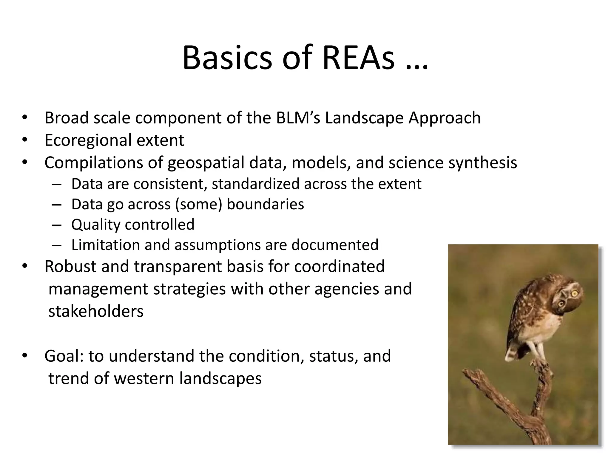
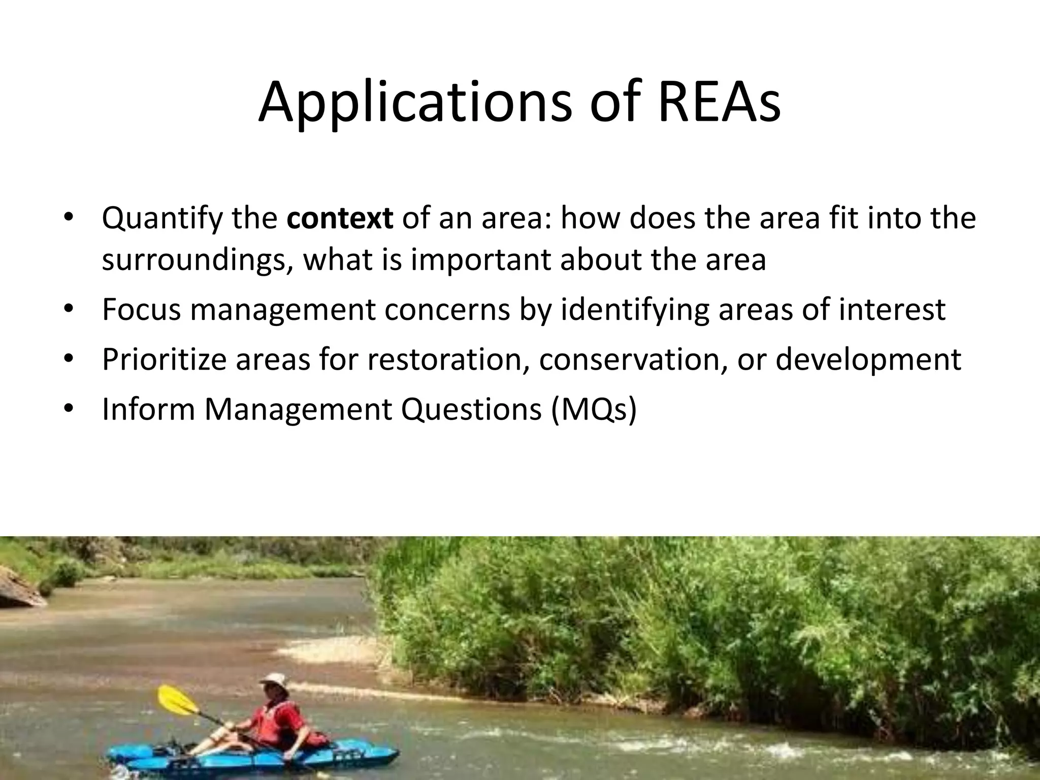
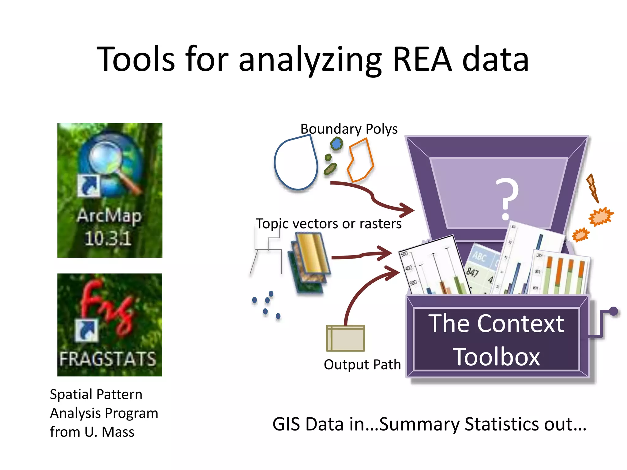
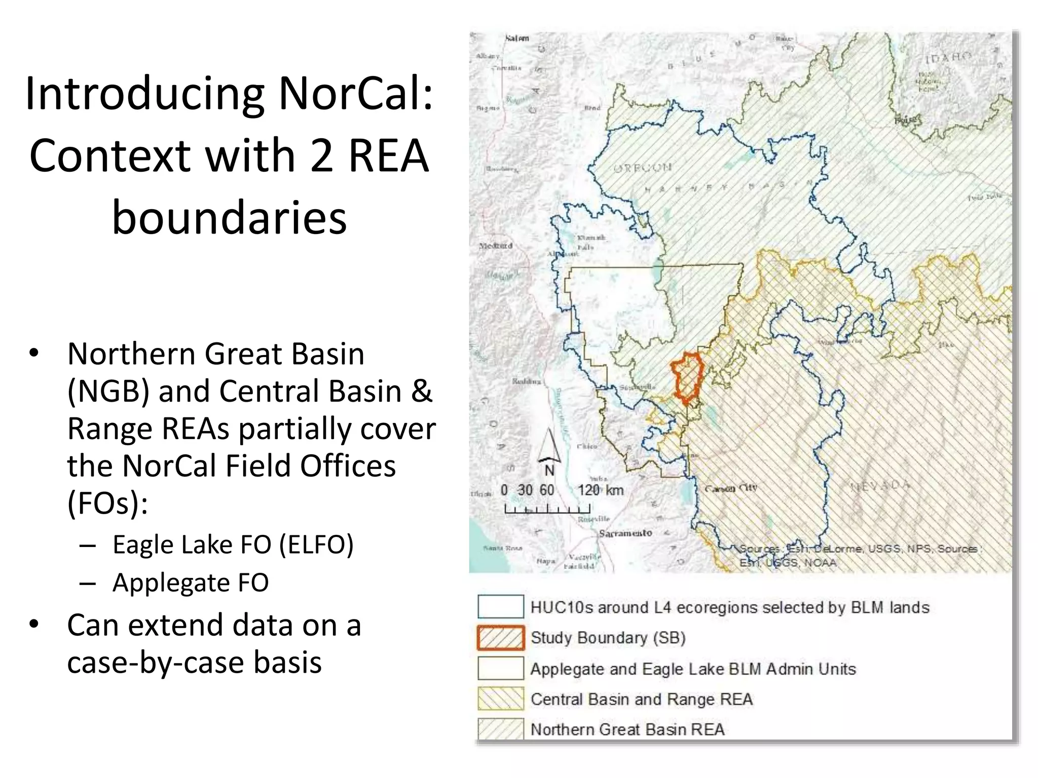
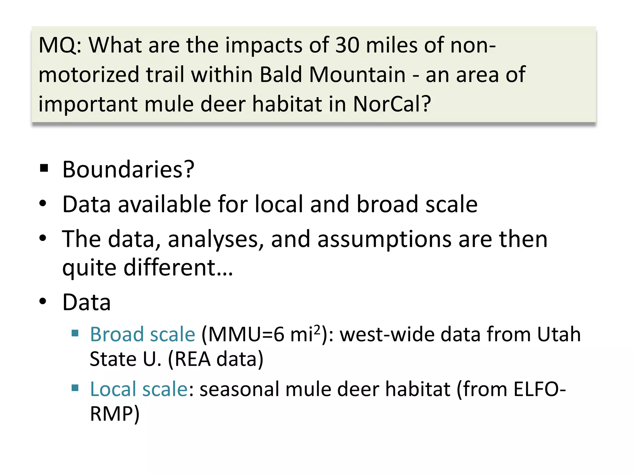
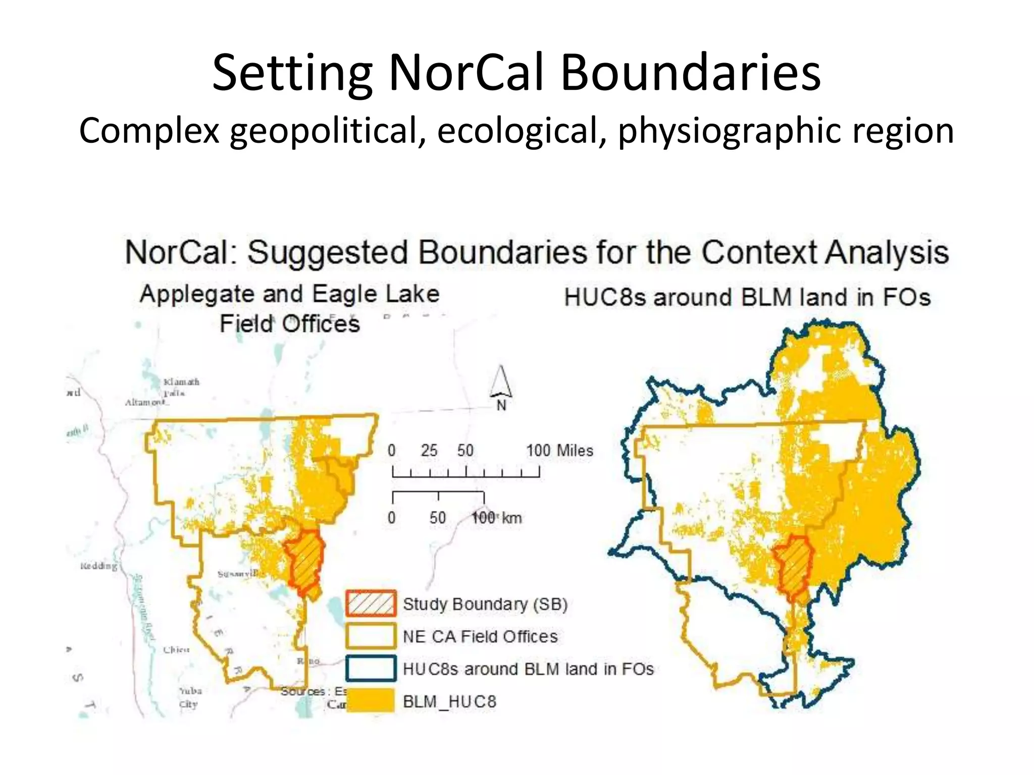
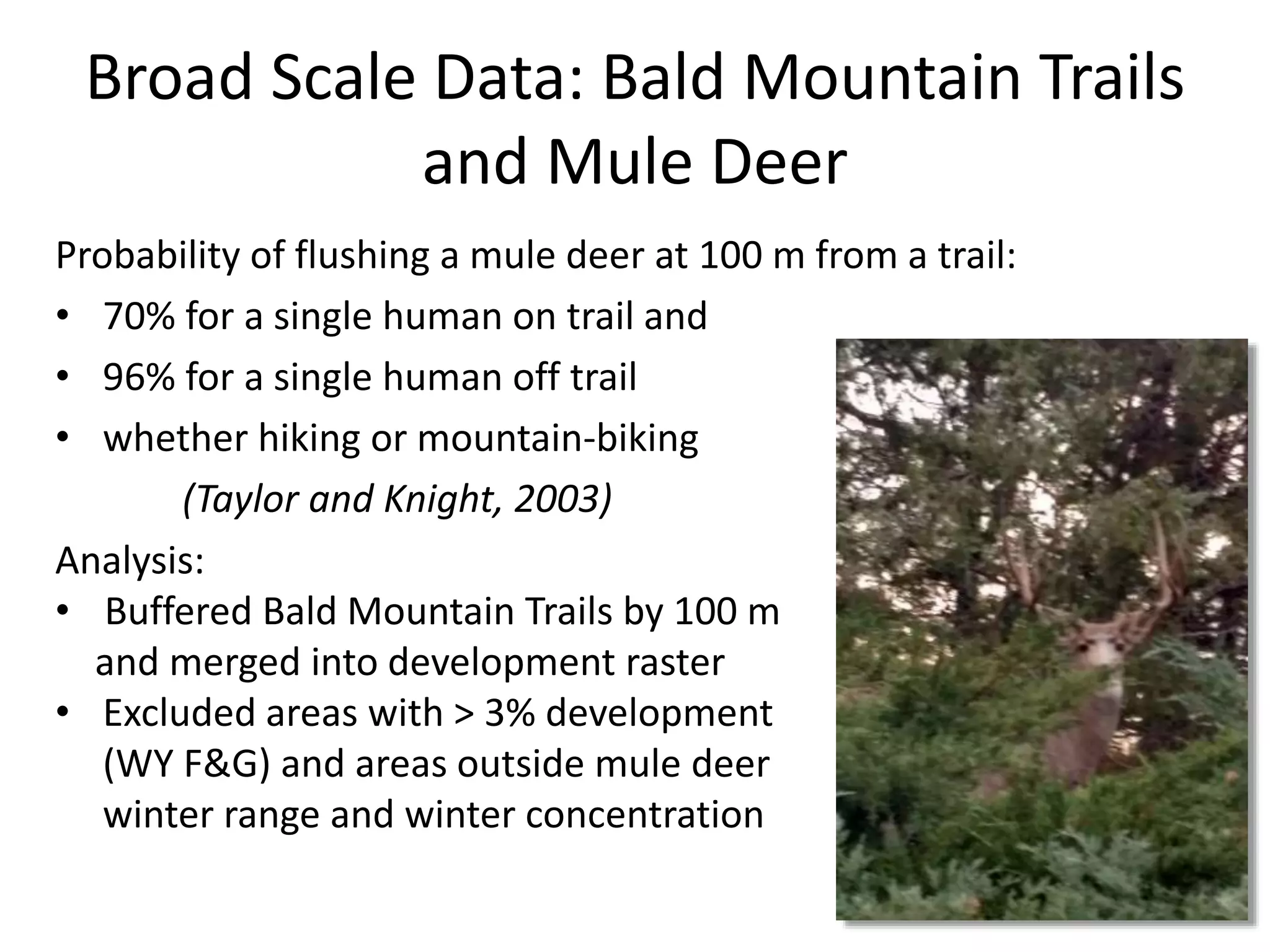
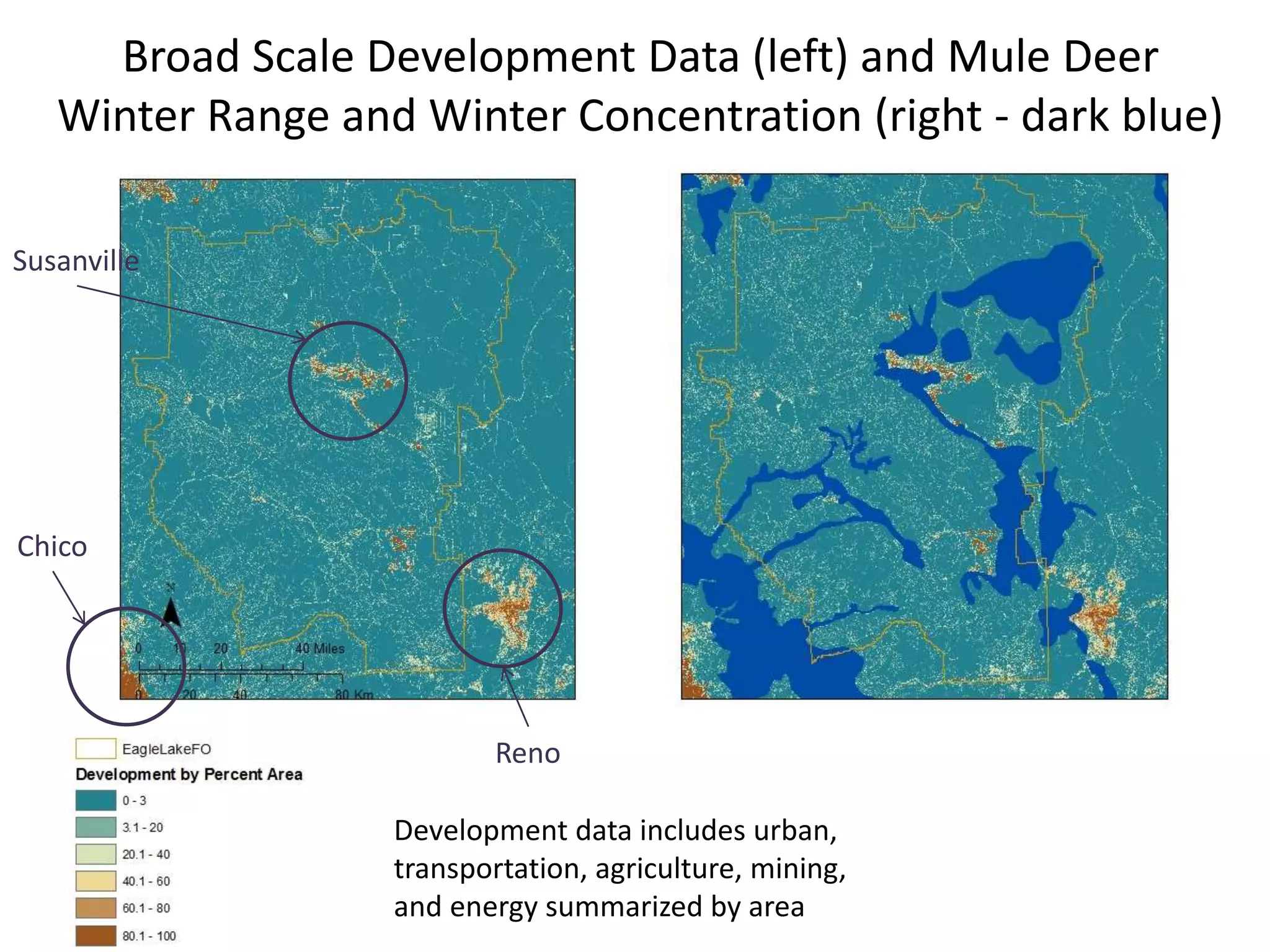
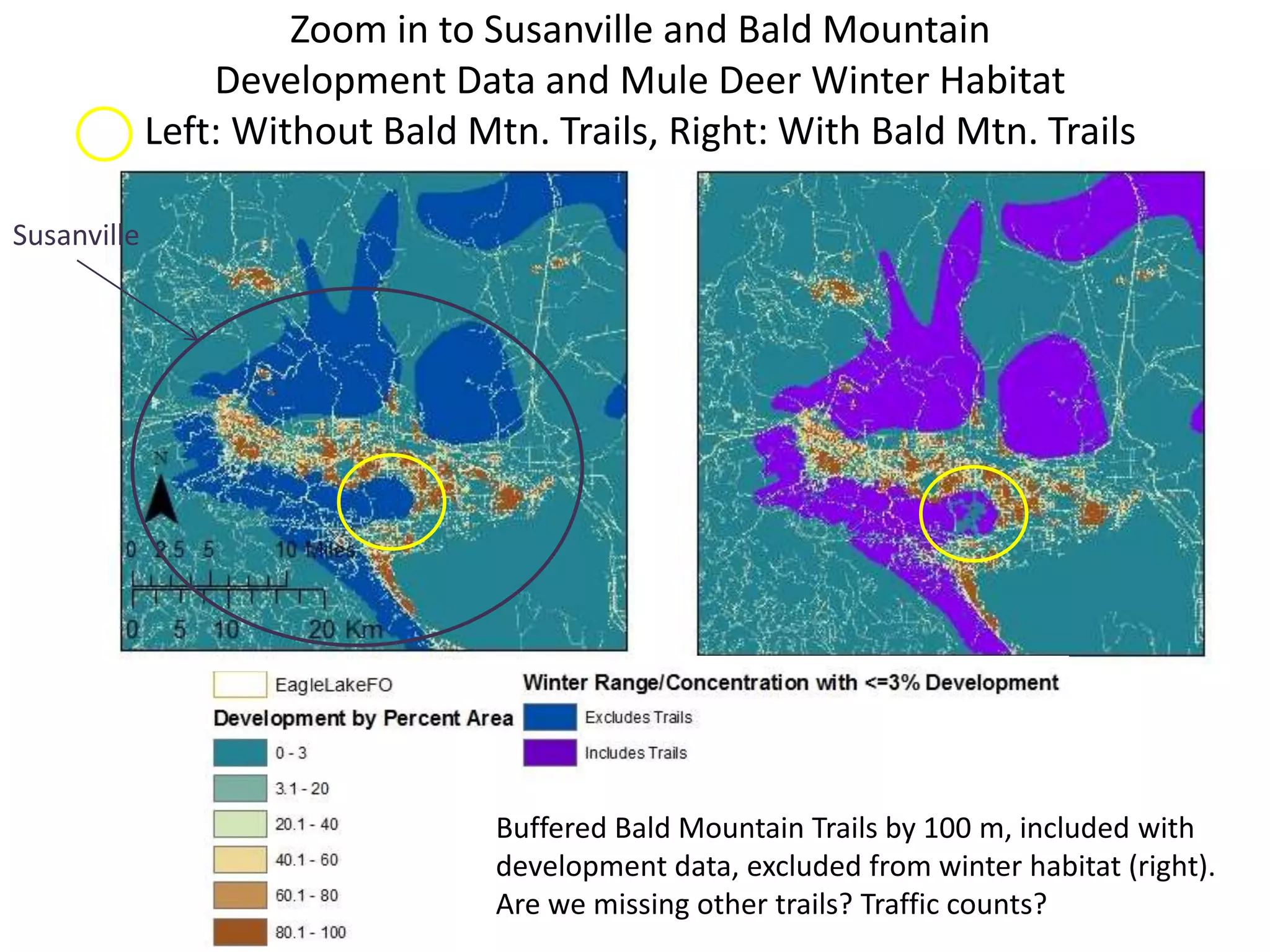
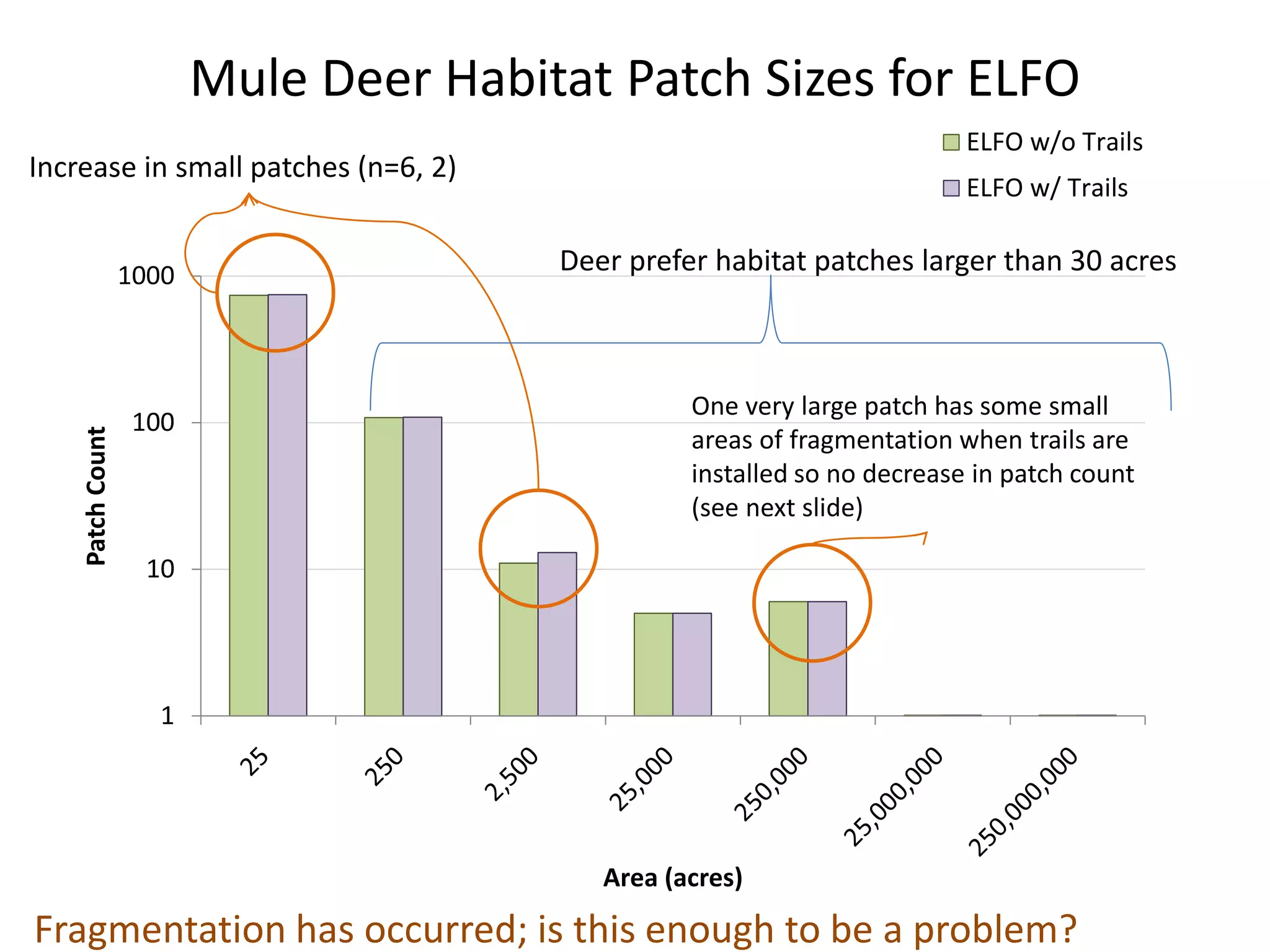
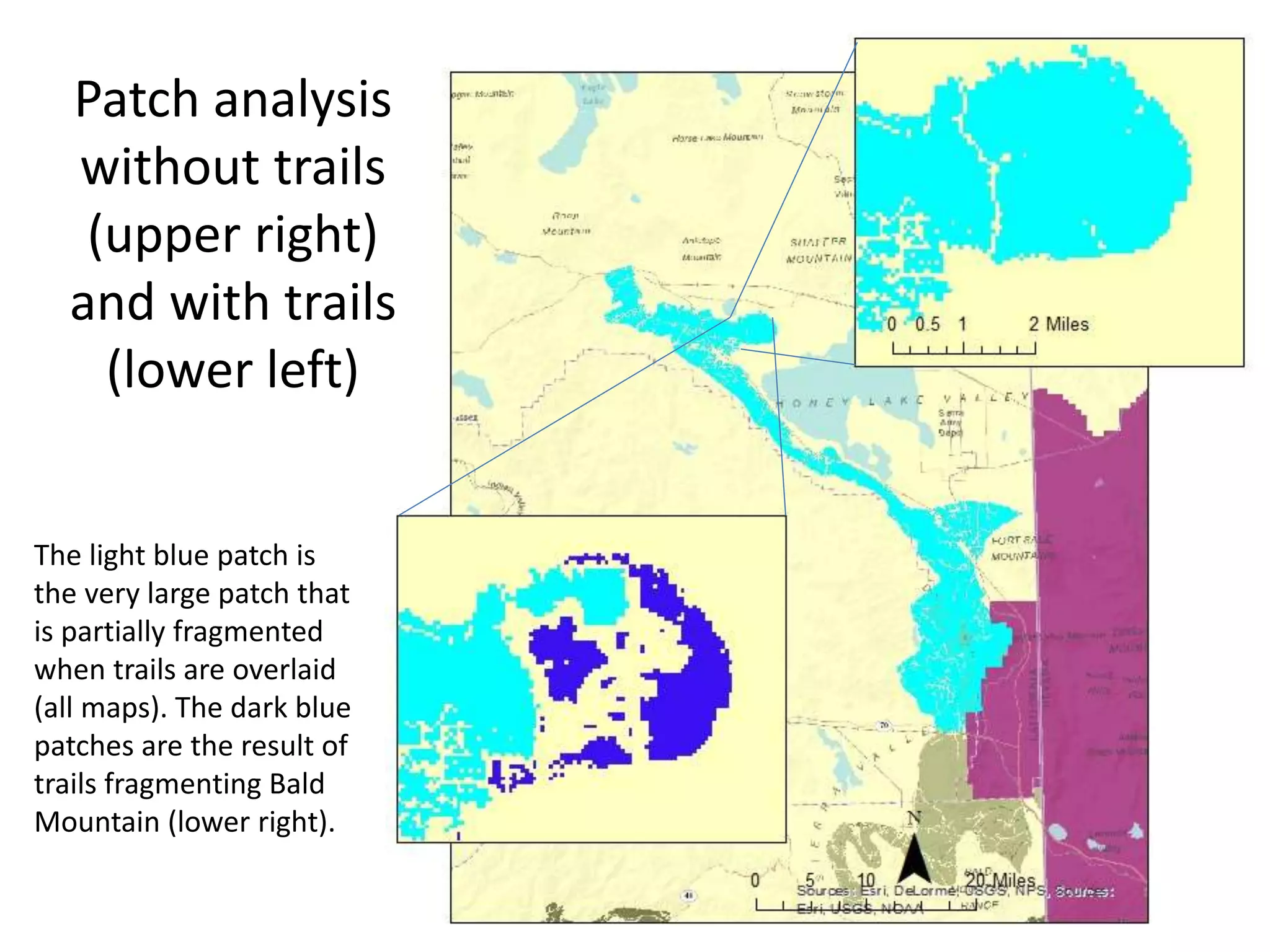
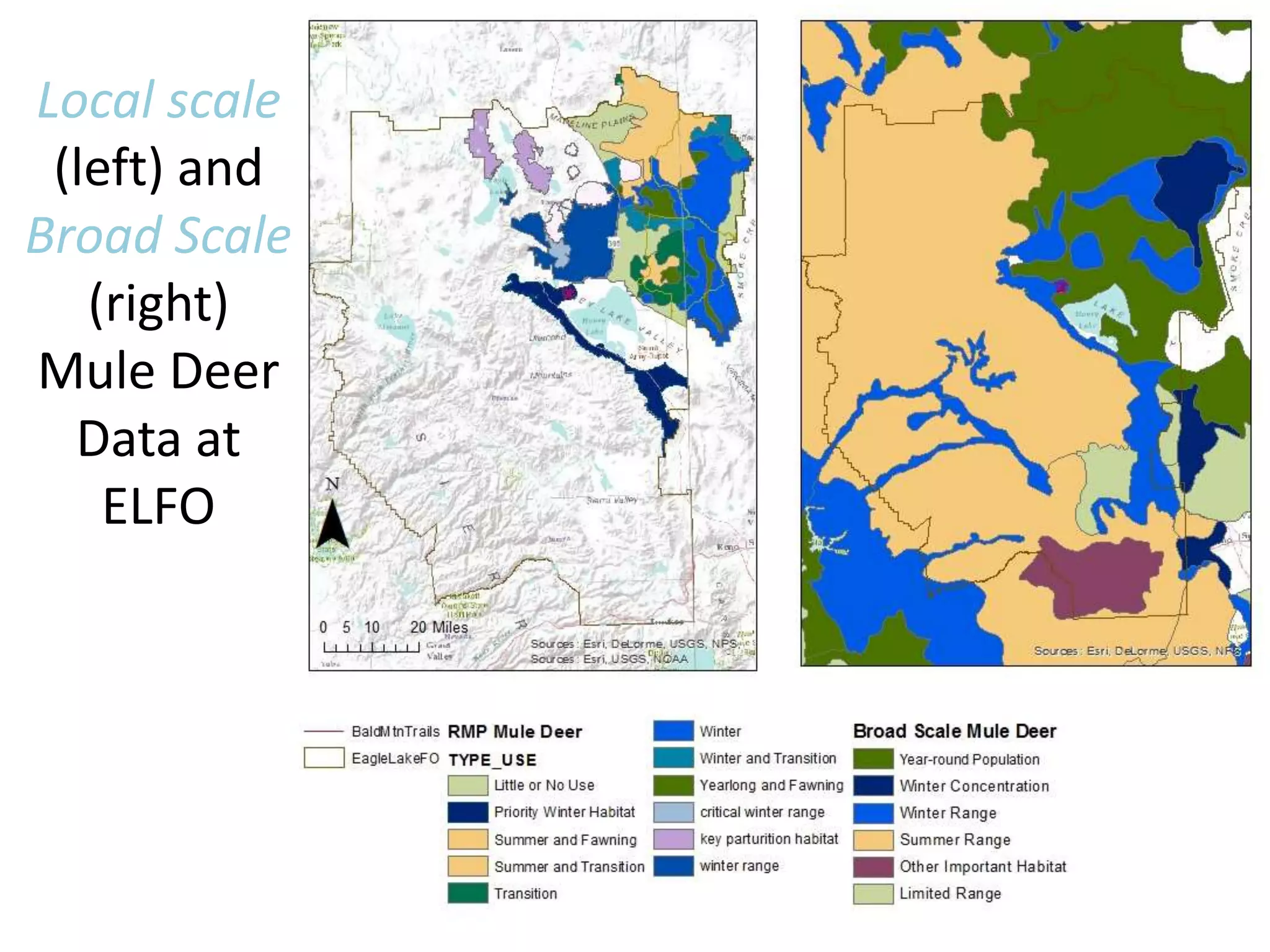
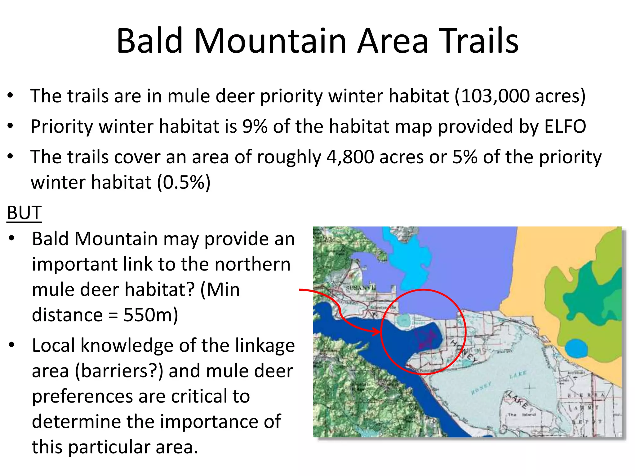

The document discusses applications of Rapid Ecoregional Assessments (REAs) conducted by the Bureau of Land Management. REAs provide standardized geospatial data across broad ecoregional extents to inform coordinated management strategies. The document examines using REA and local data to analyze the impacts of proposed non-motorized trails on mule deer habitat in Northern California. Broad-scale REA data shows the trails would have a small effect on mule deer metrics. However, local data analysis finds the trails could create a pinch point limiting connectivity, requiring on-the-ground knowledge to determine the importance.


![Vibe Coding vs. Spec-Driven Development [Free Meetup]](https://cdn.slidesharecdn.com/ss_thumbnails/vibecodingvsspecdrivendevelopment-251209105622-43f455e7-thumbnail.jpg?width=640&height=640&fit=bounds)


