1. Page 1
2011 / 2014 Aerial Imagery Displacement Analysis
Analysis of 2011 and 2014 Aerial Imagery Displacement
December 2014
Introduction:
The City of San Luis Obispo GIS Division regularly uses aerial imagery of the San Luis Obispo
County for GIS projects and analyses. Over the past three years aerial imagery collected in 2011 has
been utilized for a multitude of City projects. In 2014, aerial imagery for San Luis Obispo County was
again collected in an effort to keep GIS data current. However, a visual comparison of the aerial images
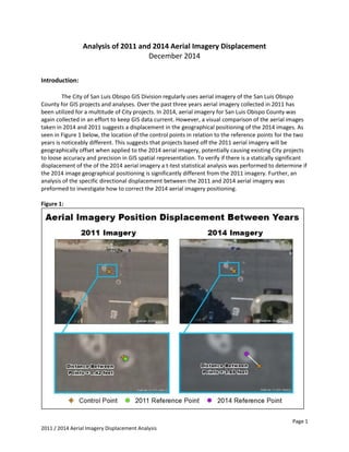
taken in 2014 and 2011 suggests a displacement in the geographical positioning of the 2014 images. As
seen in Figure 1 below, the location of the control points in relation to the reference points for the two
years is noticeably different. This suggests that projects based off the 2011 aerial imagery will be
geographically offset when applied to the 2014 aerial imagery, potentially causing existing City projects
to loose accuracy and precision in GIS spatial representation. To verify if there is a statically significant
displacement of the of the 2014 aerial imagery a t-test statistical analysis was performed to determine if
the 2014 image geographical positioning is significantly different from the 2011 imagery. Further, an
analysis of the specific directional displacement between the 2011 and 2014 aerial imagery was
preformed to investigate how to correct the 2014 aerial imagery positioning.
Figure 1:

2. Page 2
2011 / 2014 Aerial Imagery Displacement Analysis
Methods for Analysis of 2011 and 2014 Image Displacement:
To analyze the displacement between the 2011 and 2014 aerial imagery, ArcGIS was utilized to
derive and export attribute data for statistical analyses in R, a commonly used open source statistics
program. Data sources used in the analysis include the 2011 aerial imagery, 2014 aerial imagery, and a
set of control points that were collected in the field using GPS devices identifying the geographical
placement of known city monuments and landmarks. To ensure consistency in the analysis, all datasets
were projected into the NAD_1983_HARN_StatePlane_California_V_FIPS_0405_Feet coordinate systems
using the D_North_American_1983 Datum.
To quantify the difference in aerial imagery displacement between 2011 and 2014, reference
points were digitized according to the best visual estimate of where the city monuments are displayed in
the imagery (see Figure 2). This was done for both the 2011 and 2014 aerial imagery using the control
points (known GPS location of city monuments) as the orientation feature at a 1:60 map scale. If the
image poorly displayed city monument features in relation to the control points, reference points were
not digitized and these data were not used in the analysis. Of the 26 available control point locations
that exist within both the 2011 and 2014 aerial imagery, 18 locations were suitable for reference point
digitization and analysis. This provided a sample size of 36 data points used in the analysis.
Figure 2:
Once reference points were digitized, line features were generated connecting control points to
the associated reference points using the points to line data management tool for each year
respectively. The resulting line features represent the imagery displacement from the field verified
control points. GIS COGO distance and direction attributes were then calculated for each line (see Figure
3).

3. Page 3
2011 / 2014 Aerial Imagery Displacement Analysis
Figure 3:
The aerial image displacement data was then exported for statistical analysis in R to determine if
there is a statistically significant difference between the average distance displacement of the 2011 and
2014 images in relation to the known control point locations. A t-test analysis was used for the
comparison. Upon initial investigation, the data did not meet the parametric assumptions of being
normally distributed or having homogeneity of variances according to a Shapiro-wilcoxon and Bartlett
tests. To accommodate the data conditions, a non-parametric resampling t-test analysis (with
replacement) was performed using 9999 resampling iterations.
Resampling t-test Statistical Findings:
In the statistical analysis to determine if the average 2014 aerial imagery displacement is
statistically different than that of the 2011 aerial imagery, there is strong evidence showing that the
imagery displacement from control points is significantly different between the two years (t-value = -
4661.416, p-value < 0.001). Figure 4 shows a graphical representation of the resampling analysis. The t-
value from the original t-test analysis, shown by the red dot, is located in the lower tail of the histogram
representing strong evidence of significant statistical findings.

4. Page 4
2011 / 2014 Aerial Imagery Displacement Analysis
Figure 4:
Methods for Analysis of 2014 Image Adjustment Potential:
Given the results from the previous analysis, an investigation as to how the 2014 aerial images
might be adjusted to better fit GIS projects based off the 2011 aerial images was conducted. If achieved,
GIS projects based off the 2011 imagery might be applied to the more current 2014 imagery without
loosing much data precision and accuracy. This was completed using ArcGIS and excel for descriptive
statistical comparison.
To begin the analysis, line features connecting both the 2011 and 2014 reference points at each
location were generated and COGO distance and direction attributes were calculated. The distance and
direction attributes were then exported to excel where a mean and median value was calculated
representing the average and median distance and directional offset of the 2014 imagery from the 2011
imagery geographical positioning. These values were then used to shift the 2014 reference points and
evaluate the adjusted fit of the 2014 aerial imagery in relation to the 2011 aerial imagery.
To shift the 2014 reference points, the construct 2-point line edit tool was utilized to create a
new line with the specified distance and direction of both the mean and median 2014 offset values.
Then the feature vertices to points tool was applied creating new points at the end of each of the new
line features (see Figure 5). These points represent the geographical location of where the 2014
reference points would be if the 2014 aerial imagery was shifted using the mean or median 2014
distance and direction offset values.
Original t.value = -4661.416
p-value < 0.001
Original
t.value

5. Page 5
2011 / 2014 Aerial Imagery Displacement Analysis
Figure 5:
Finally, line features were created using the points to line tool and COGO Distance attributes
were calculated to analyze the distance from these adjusted reference points to the 2011 aerial imagery
reference points (see Figure 6). These data were then exported to excel where the average distance
from 2011 reference points were calculated for each of the 2014 adjusted offset locations to gain an
understanding of which adjustment measures would best improve the 2014 aerial imagery fit to the
2011 aerial imagery.
Figure 6:
2014 Image Adjustment Potential Findings and Discussion:
When determining the direction and distance to potentially shift the 2014 aerial imagery to
better fit the 2011 imagery, the mean and median offset distance and direction of the 2014 imagery
from the 2011 imagery was calculated. These values are displayed in Table 1 below and were used to
further analyze how the 2014 Imagery might better fit the 2011 Imagery if geographically shifted.
Concerning the direction values, the data represented the direction from the 2011 reference point to

6. Page 6
2011 / 2014 Aerial Imagery Displacement Analysis
the 2014 reference point. Since we want to know how to shift the 2014 reference points, not the 2011
reference points, 180 degrees was subtracted from the mean and median figures to correctly identify
the directional shift of the 2014 reference points. These values are reported in Table 1.
Table 1:
2014 Aerial Imagery Offset from 2011 Aerial Imagery
Direction (North
Azimuth Bearing)
Distance (ft)
Mean Offset 135.83 3.87
Median Offset 141.32 3.94
Once all the 2014 reference points were shifted according to the mean and median offset
distance and direction values, the distance between the adjusted 2014 reference points to the 2011
reference points was calculated. An average of these distances was calculated to understand which
offset adjustment values best fit the 2011 aerial imagery. These averages are reported in Table 2 below.
Table 2:
Average Distance of Adjusted 2014 Aerial Imagery from
2011 Aerial Imagery
Average Distance (ft)
Mean Offset Adjustment 1.16
Median Offset Adjustment 1.11
The results of this assessment show that the Median direction and offset adjustment is a slightly
better fit to the 2011 aerial imagery with an average distance from the 2011 reference points of 1.11
feet. This is much improved to the original average distance from the 2011 reference points of 3.87 feet
(Table 1). However, it is important to recognize that using an average value as the assessment factor in
improved fit between the adjusted 2014 imagery reference points and the 2011 imagery reference
points means that some 2014 adjusted reference points will be closer to the 2011 reference points while
others will be further away. The stacked bar graph in Figure 7 shows the overall impact of the 2014
adjustment on the entire data set.
Overall the distance from the 2011 reference points is much improved for both the adjusted
mean and median offset values, with the exception of data point 1. Considering the increased distance
from the 2011 reference point for this data point, it is possible that the 2014 reference point was
improperly digitized for this particular point due to the subjective nature of the digitization process.
When looking at the specific improvement in distance to the 2011 reference points according to the
mean or median adjustments, both values are a better fit in some cases while not in others. This means
that either the 2014 mean or median adjustment value could be likely be used with similar outcome.

7. Page 7
2011 / 2014 Aerial Imagery Displacement Analysis
Figure 7:
Conclusions:
In conclusion, this study found that the geographical positioning of the 2014 aerial imagery is
significantly different from the 2011 aerial imagery in relation to known control points. When assessing
if the 2014 aerial imagery could be shifted to better fit the 2011 aerial imagery to maintain accuracy and
precision of GIS projects based off the 2011 imagery, the 2014 median offset direction and distance
values produced the best fit. However, there is still an average offset distance of 1.11 feet from the 2011
reference points after the 2014 median offset adjustment. If this is an acceptable offset distance from
the 2011 aerial imagery, then the 2014 aerial imagery should be shifted according to the median offset
value. If not, further analysis should be made to determine a better method for improving the 2014
aerial imagery displacement.
0
1
2
3
4
5
6
1 2 3 4 5 6 7 8 9 10 11 12 13 14 15 16 17 18
Distancefrom2011ReferencePoint(ft)
Reference Point ID
2014 Aerial Image Adjustment Impact to Reference Points
Original 2014 Point Distance
Adjusted Distance (Mean)
Adjusted Distance (Median)