1_ Introduction Python.pptx python is a data

INDIAN INSTITUTE OF TECHNOLOGY ROORKEE
Lecture 1: Python – Fundamentals
Dr. A. Ramesh
DEPARTMENT OF MANAGEMENT
IIT ROORKEE

2
2
Learning objectives
1. Installing Python
2. Fundamentals of Python
3. Data Visualisation
2

3
3
Python Installation Process
Installation Process –
Step 1: Type https://www.anaconda.com at the address bar of web
browser.
Step 2: Click on download button
Step 3: Download python 3.8 version for windows OS
Step 4: Double click on file to run the application
Step 5: Follow the instructions until completion of installation process
3

4
4
Installation Process –
Step 1: Type https://www.anaconda.com at the address bar of web browser.
4

5
5
Step 2: Click on download button
5

6
6
Step 3: Download python 3.8 version for windows OS
6

7
7
Step 4: Double click on the downloaded file to run the application
7

8
8
8

9
9
9

10
10
10

11
11
11

12
12
12

13
13
13

14
14
14

15
15
15

16
16
16

17
17
Why Jupyter NoteBook?
17
Why?
• Edit code on web browser
• Easy in documentation
• Easy in demonstration
• User- friendly Interface

18
18
Python and Jupyter
18
Python Programming Language Jupyter Application
Software Package contains both
python and jupyter application

20
20
About Jupyter NoteBook
20
Cell -> Access using Enter Key

21
21
21
Input Field -> Green color indicates edit mode
Blue color indicates command mode

22
22
22
-> It contains documentation
-> Text not executed as code

23
23
About Jupyter Notebook
• Command mode allow to edit notebook as whole
• To close edit mode (Press Escape key)
• Execution (Three ways)
• Comment line is written preceding with # symbol.
23
o Ctrl +Enter (Output field can not be modified)
o Shift +Enter (Output field is modified)
o Run button on Jupyter interface

24
24
About Jupyter Notebook
• Important shortcut keys
24
o A -> To create cell above
o B -> To create cell below
o D + D -> For deleting cell
o M -> For markdown cell
o Y -> For code cell

25
25
Fundamentals of Python
• Loading a simple delimited data file
• Counting how many rows and columns were loaded
• Determining which type of data was loaded
• Looking at different parts of the data by subsetting rows and columns
25

Importing Different Files in Jupyter Notebook
• Importing text file
26

• Importing tablular file
27

• Importing excel file
28

• Importing Zip file
29

• Importing PDF file
30

32
32
Loading a simple delimited data file
32

34
34
• head method shows us only the first 5 rows
34

35
35
Get the number of rows and columns
35

37
37
get the dtype of each column
37

38
38
Pandas Types Versus Python Types
38

39
39
get more information about data
39

40
40
Looking at Columns, Rows, and Cells
• # get the country column and save it to its own variable
40

41
41
# show the first 5 observations
41

42
42
# show the last 5 observations
42

43
43
# Looking at country, continent, and year
43

45
45
Looking at Columns, Rows, and Cells
• Subset Rows by Index Label: loc
45

46
46
get the first row
• Python counts from 0
46

47
47
• # get the 100th row
# Python counts from 0
47

49
49
Subsetting Multiple Rows
• # select the first, 100th, and 1000th rows
49

50
50
Subset Rows by Row Number: iloc
• # get the 2nd row
50

51
51
• get the 100th row
51

52
52
• # using -1 to get the last row
52

53
53
With iloc, we can pass in the -1 to get the last row—something we couldn’t do with loc.
53

54
54
• # get the first, 100th, and 1000th rows
54

55
55
Subsetting Columns
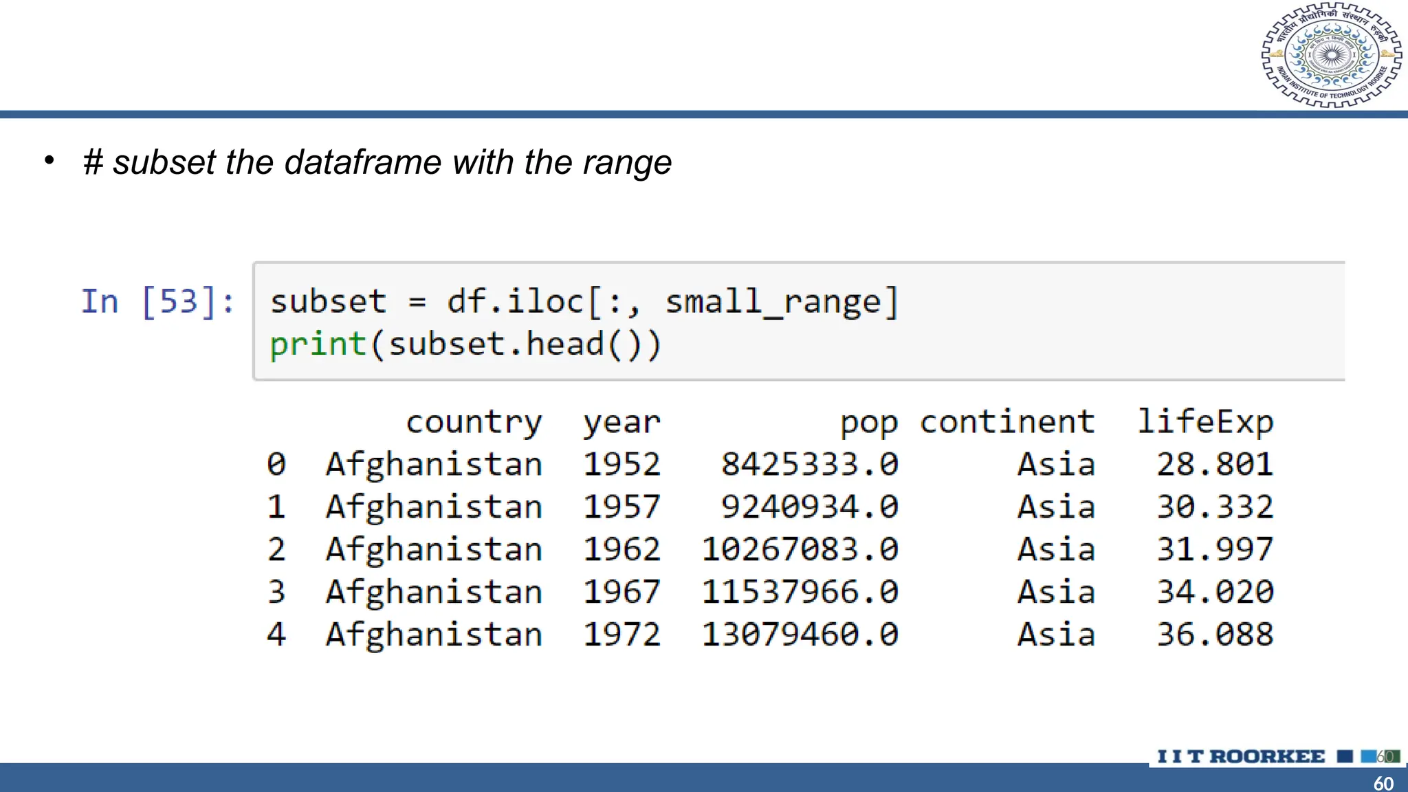
• The Python slicing syntax uses a colon, :
• If we have just a colon, the attribute refers to everything.
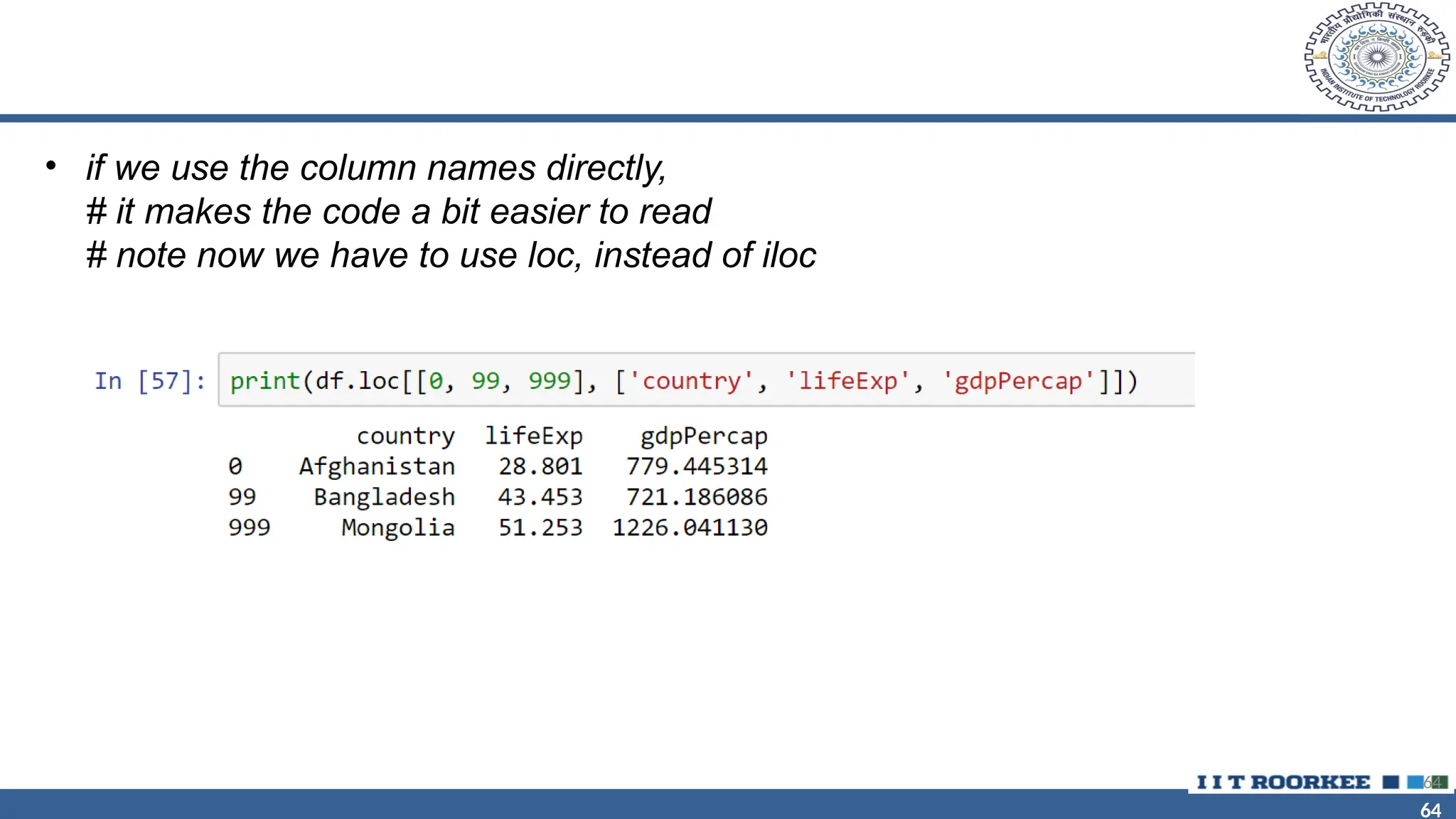
• So, if we just want to get the first column using the loc or iloc syntax,
we can write something like df.loc[:, [columns]] to subset the column(s).
55

56
56
• # subset columns with loc
# note the position of the colon
# it is used to select all rows
56

58
58
• # subset columns with iloc
• # iloc will alow us to use integers
• # -1 will select the last column
58

59
59
Subsetting Columns by Range
• # create a range of integers from 0 to 4 inclusive
59

60
60
• # subset the dataframe with the range
60

61
61
Subsetting Rows and Columns
• # using loc
61

63
63
Subsetting Multiple Rows and Columns
• #get the 1st, 100th, and 1000th rows
# from the 1st, 4th, and 6th columns
63

64
64
• if we use the column names directly,
# it makes the code a bit easier to read
# note now we have to use loc, instead of iloc
64

67
67
Grouped Means
• # For each year in our data, what was the average life expectancy?
# To answer this question,
# we need to split our data into parts by year;
# then we get the 'lifeExp' column and calculate the mean
67

70
70
• If you need to “flatten” the dataframe, you can use the
reset_index method.
70

71
71
Grouped Frequency Counts
• use the nunique to get counts of unique values on a Pandas Series.
71

74
74
Visual Representation of the Data
• Histogram -- vertical bar chart of frequencies
• Frequency Polygon -- line graph of frequencies
• Ogive -- line graph of cumulative frequencies
• Pie Chart -- proportional representation for categories of a whole
• Stem and Leaf Plot
• Pareto Chart
• Scatter Plot
74

75
75
Methods of visual presentation of data
• Table
75
1st Qtr 2nd Qtr 3rd Qtr 4th Qtr
East 20.4 27.4 90 20.4
West 30.6 38.6 34.6 31.6
North 45.9 46.9 45 43.9

76
76
• Graphs
76
0
10
20
30
40
50
60
70
80
90
East
West
North

77
77
• Pie chart
77
1st Qtr
2nd Qtr
3rd Qtr
4th Qtr

78
78
• Multiple bar chart
78
0 20 40 60 80 100
1st Qtr
2nd Qtr
3rd Qtr
4th Qtr
North
West
East

79
79
• Simple pictogram
79
0
20
40
60
80
100
East
North
West

80
80
Frequency distributions
• Frequency tables
80
Class Interval Frequency Cumulative Frequency
< 20 13 13
<40 18 31
<60 25 56
<80 15 71
<100 9 80
Observation Table

81
81
Frequency diagrams
Frequency
0
5
10
15
20
25
30
< 20 <40 <60 <80 <100
Frequency
81
Frequency
0
5
10
15
20
25
30
< 20 <40 <60 <80 <100
Frequency
Cumulative Frequency
0
10
20
30
40
50
60
70
80
90
< 20 <40 <60 <80 <100
Cumulative Frequency

82
82
Histogram
82
Class Interval
Frequency
20-under 30 6
30-under 40 18
40-under 50 11
50-under 60 11
60-under 70 3
70-under 80 1
0
10
20
0 10 20 30 40 50 60 70 80
Years
Frequency

83
83
Histogram Construction
83
Class Interval Frequency
20-under 30 6
30-under 40 18
40-under 50 11
50-under 60 11
60-under 70 3
70-under 80 1
0
10
20
0 10 20 30 40 50 60 70 80
Years
Frequency

84
84
Frequency Polygon
84
Class IntervalFrequency
20-under 30 6
30-under 40 18
40-under 50 11
50-under 60 11
60-under 70 3
70-under 80 1
0
10
20
0 10 20 30 40 50 60 70 80
Years
Frequency

85
85
Ogive
Cumulative
20-under 30 6
30-under 40 24
40-under 50 35
50-under 60 46
60-under 70 49
70-under 80 50
85
0
20
40
60
0 10 20 30 40 50 60 70 80
Years
Frequency

86
86
Relative Frequency Ogive
Cumulative
Relative
20-under 30 .12
30-under 40 .48
40-under 50 .70
50-under 60 .92
60-under 70 .98
70-under 80 1.00
86
0.00
0.10
0.20
0.30
0.40
0.50
0.60
0.70
0.80
0.90
1.00
0 10 20 30 40 50 60 70 80
Years
Cumulative
Relative
Frequency

87
87
Pareto Chart
87
0
10
20
30
40
50
60
70
80
90
100
Poor
Wiring
Short in
Coil
Defective
Plug
Other
Frequency
0%
10%
20%
30%
40%
50%
60%
70%
80%
90%
100%

88
88
Scatter Plot
Registered Vehicles (1000's) Gasoline Sales (1000's of Gallons)
5 60
15 120
9 90
15 140
7 60
0
100
200
0 5 10 15 20
RegisteredVehicles
Gasoline
Sales
88

89
89
Principles of Excellent Graphs
• The graph should not distort the data
• The graph should not contain unnecessary adornments (sometimes
referred to as chart junk)
• The scale on the vertical axis should begin at zero
• All axes should be properly labeled
• The graph should contain a title
• The simplest possible graph should be used for a given set of data

90
90
Graphical Errors: Chart Junk
1960: $1.00
1970: $1.60
1980: $3.10
1990: $3.80
Minimum Wage
Bad Presentation
Minimum Wage
0
2
4
1960 1970 1980 1990
$
 Good Presentation

91
91
Graphical Errors:
Compressing the Vertical Axis
Good Presentation
Quarterly Sales Quarterly Sales
Bad Presentation
0
25
50
Q1 Q2 Q3 Q4
$
0
100
200
Q1 Q2 Q3 Q4
$


92
92
Graphical Errors: No Zero Point on the Vertical Axis
Monthly Sales
36
39
42
45
J F M A M J
$
Graphing the first six months of sales
Monthly Sales
0
39
42
45
J F M A M J
$
36
Good Presentations
Bad Presentation

1_ Introduction Python.pptx python is a data

More Related Content

Similar to 1_ Introduction Python.pptx python is a data

Recently uploaded

1_ Introduction Python.pptx python is a data