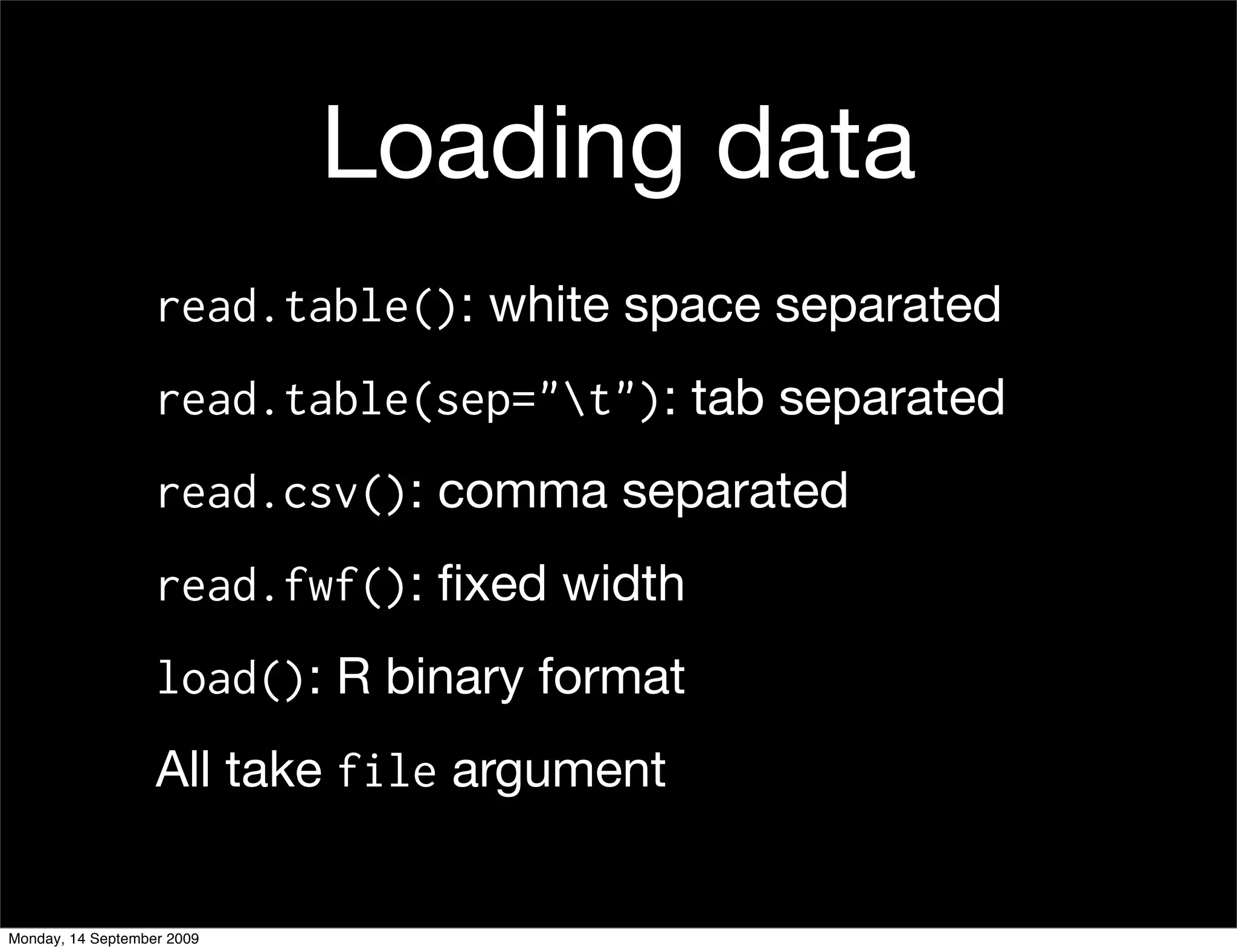
Downloaded 42 times


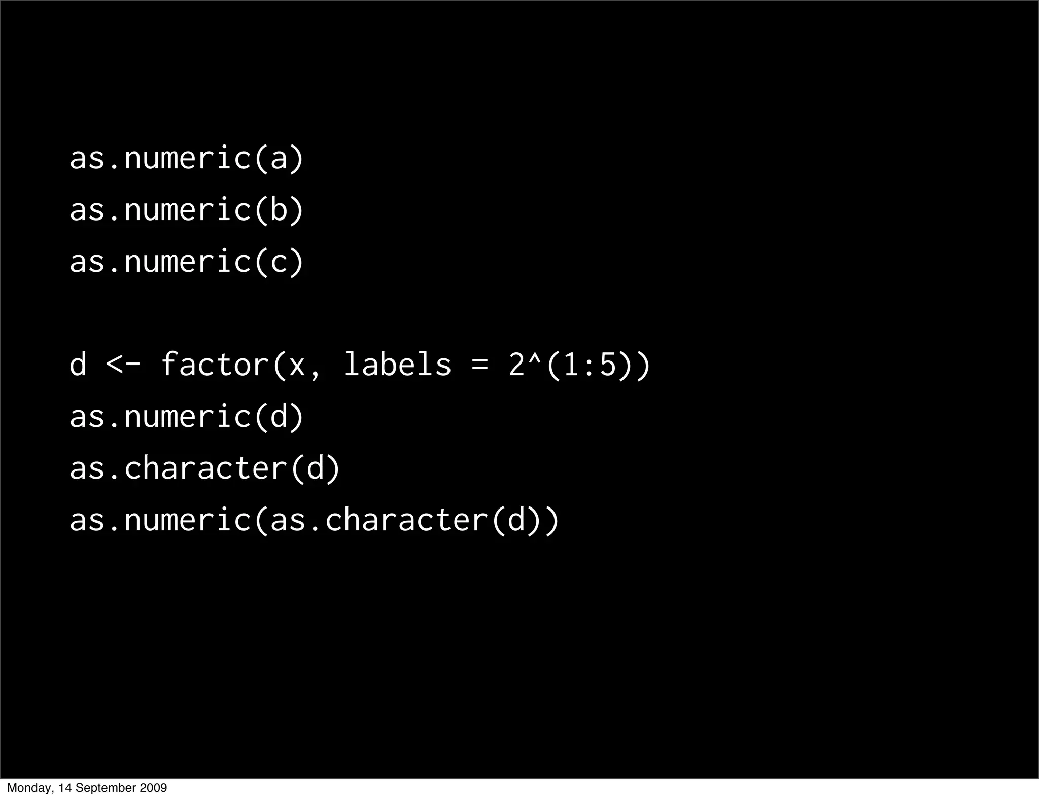
![# Creating a factor
x <- sample(5, 20, rep = T)
a <- factor(x)
b <- factor(x, levels = 1:10)
c <- factor(x, labels = letters[1:5])
levels(a); levels(b); levels(c)
table(a); table(b); table(c)
Monday, 14 September 2009](https://image.slidesharecdn.com/06-data-090914140203-phpapp01/75/06-Data-19-2048.jpg)
![# Subsets
b2 <- b[1:5]
levels(b2)
table(b2)
# Remove extra levels
b2[, drop=T]
factor(b2)
# Convert to character
b3 <- as.character(b)
table(b3)
table(b3[1:5])
Monday, 14 September 2009](https://image.slidesharecdn.com/06-data-090914140203-phpapp01/75/06-Data-20-2048.jpg)
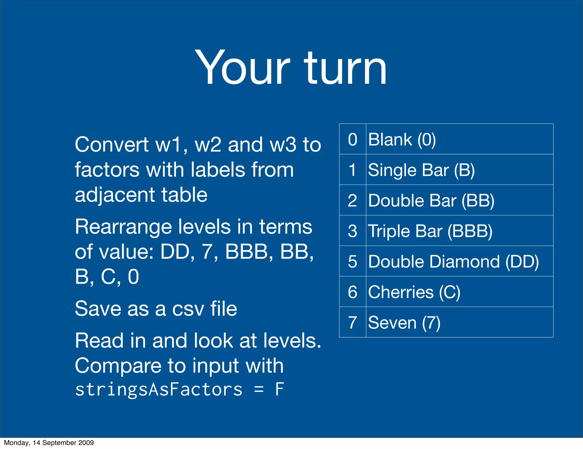
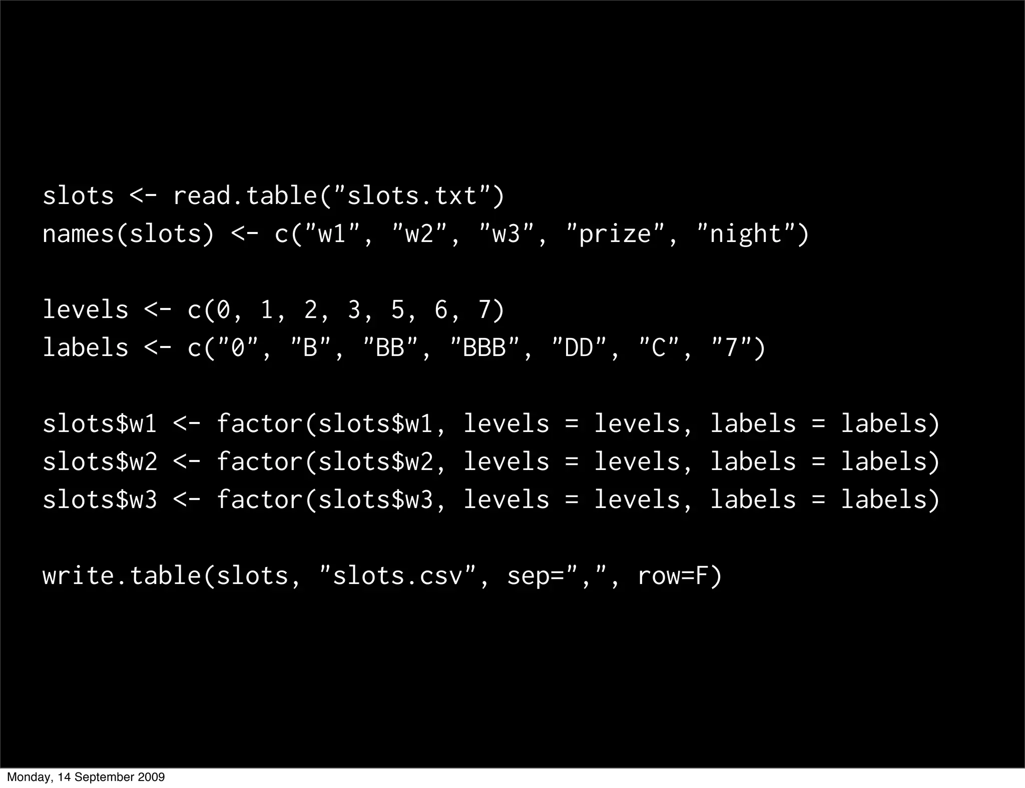

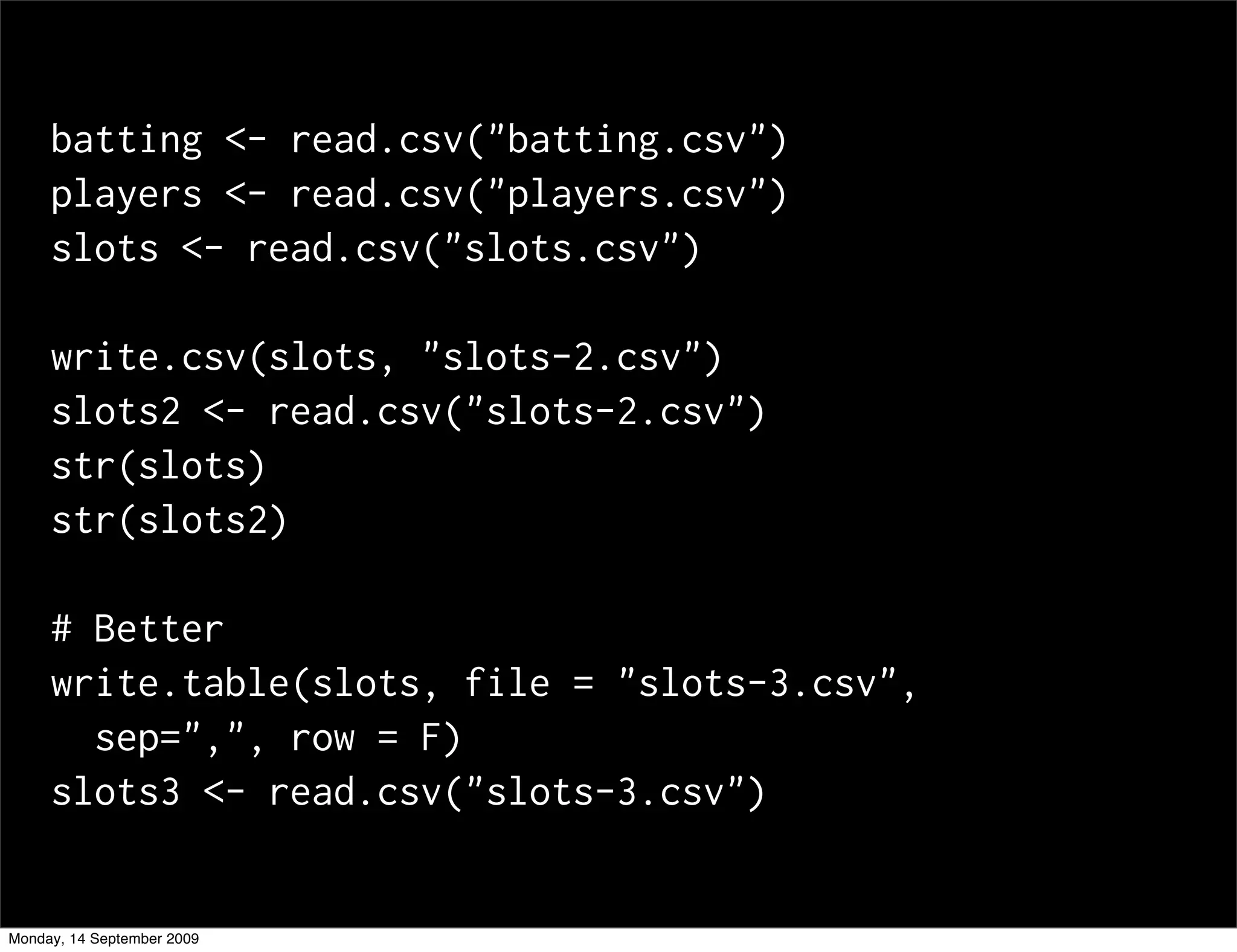
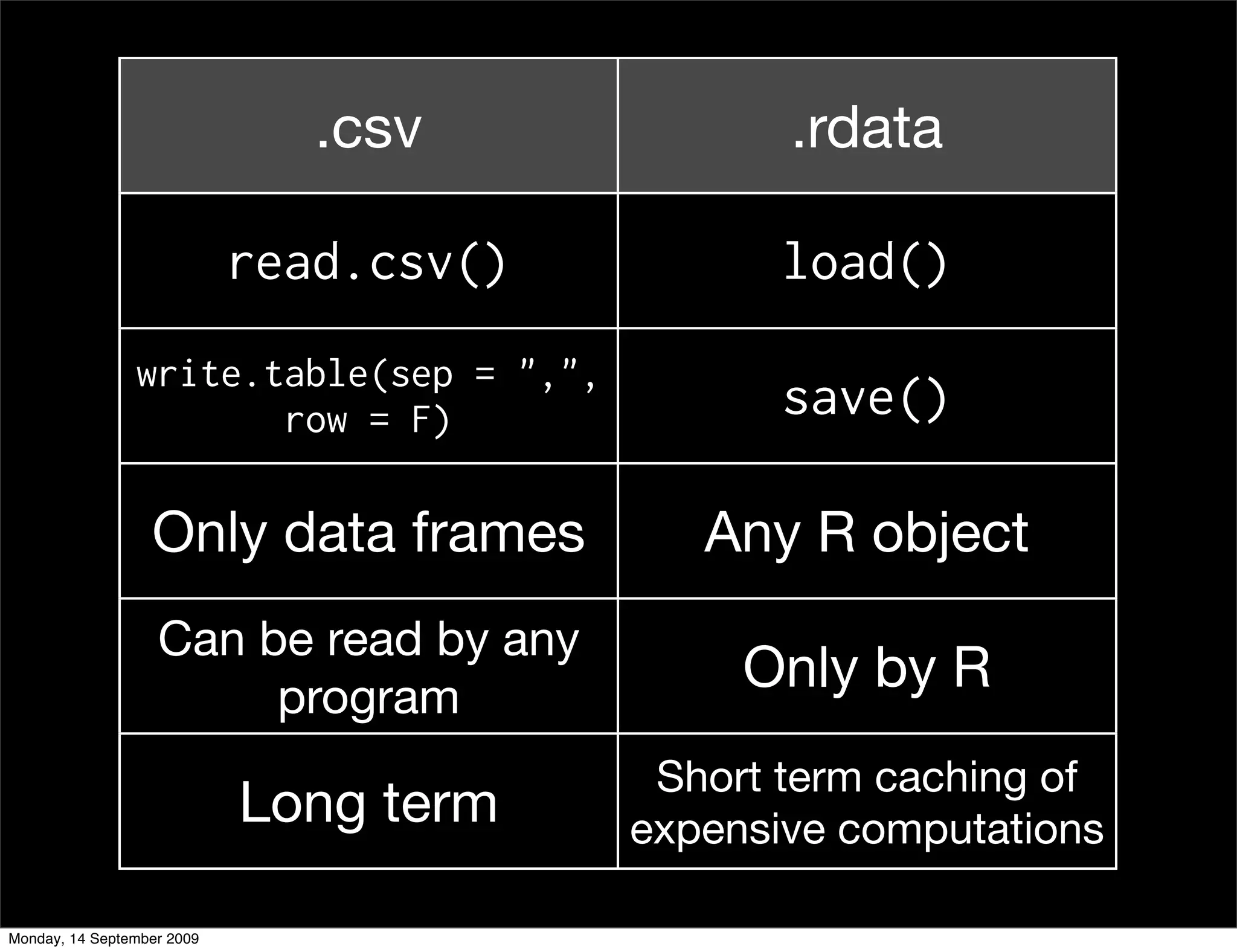
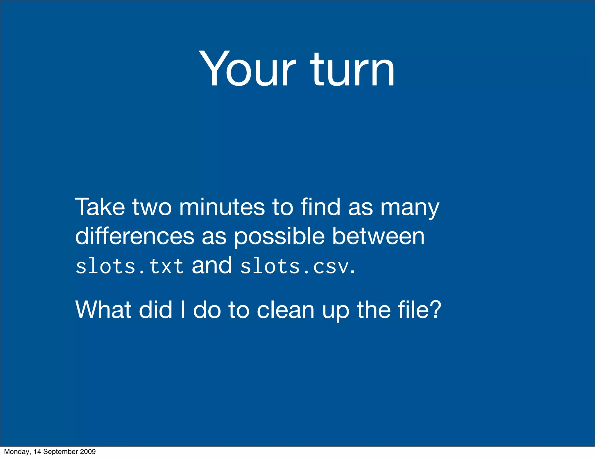
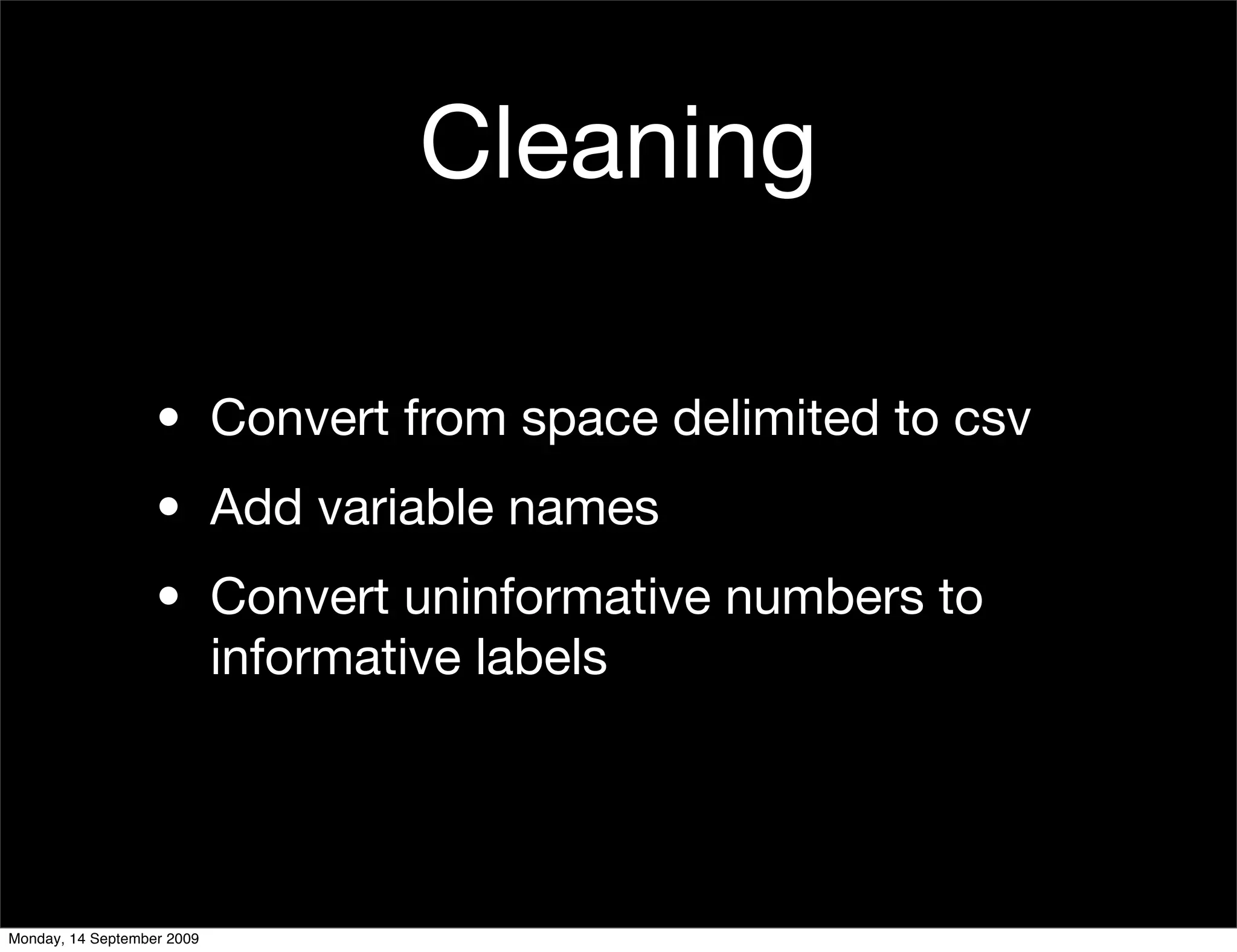
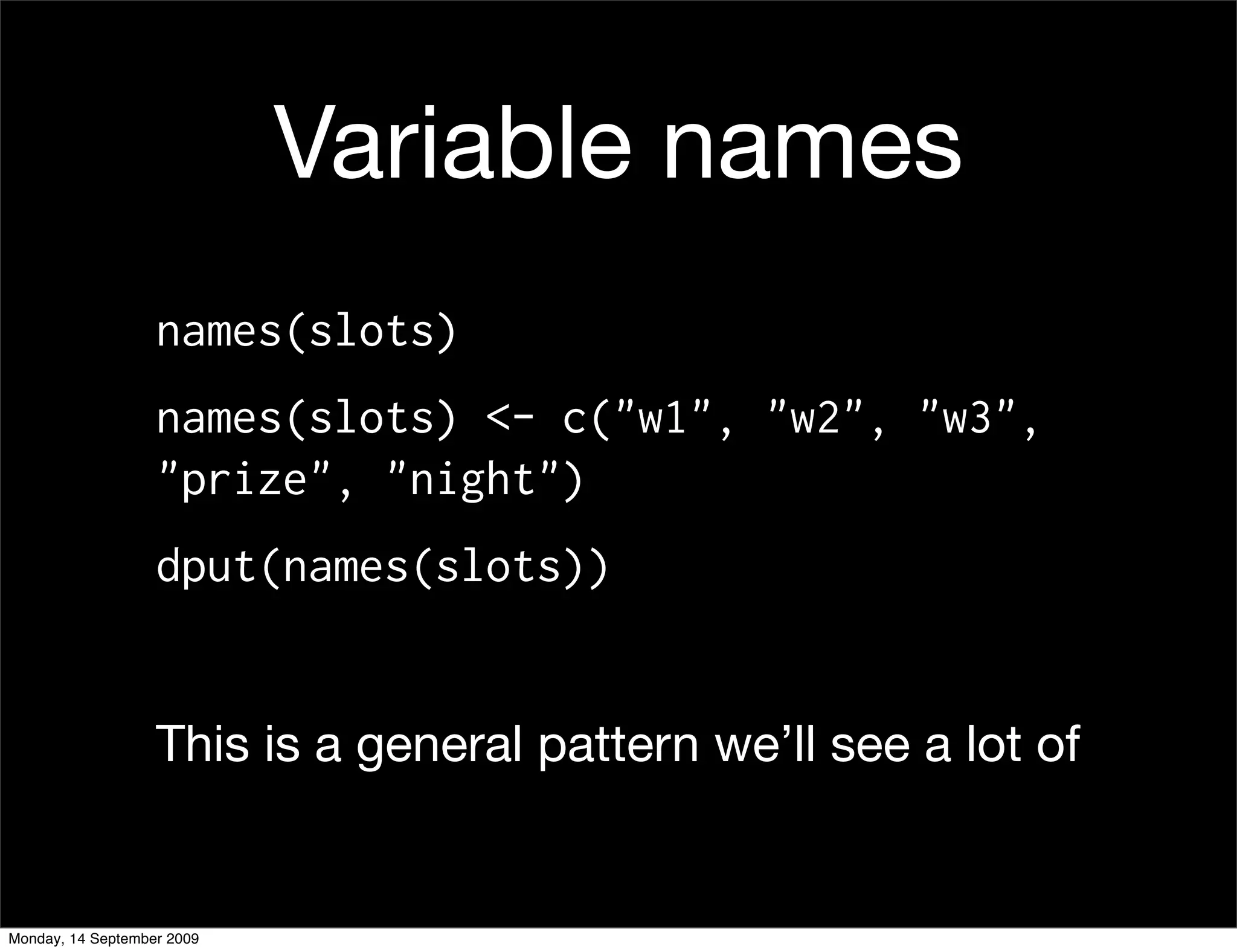
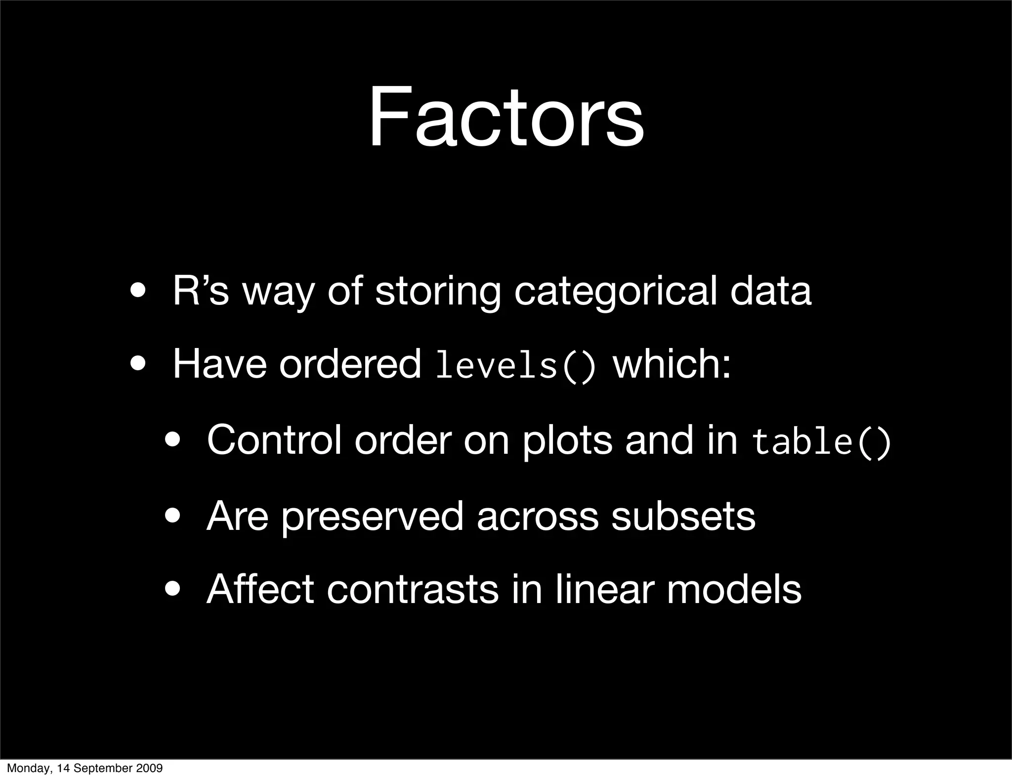
- The document discusses loading and cleaning data, including using functions like read.csv() and write.csv() to load and save CSV files in R. - It also covers creating and working with factors in R, including setting levels and labels when converting variables to factors. - An example is given of converting variables in a slots data set to factors and reordering the levels.


![Vibe Coding vs. Spec-Driven Development [Free Meetup]](https://cdn.slidesharecdn.com/ss_thumbnails/vibecodingvsspecdrivendevelopment-251209105622-43f455e7-thumbnail.jpg?width=640&height=640&fit=bounds)


