This document introduces the China's Energy Requirements and CO2 Emissions Analysis System (CErCmA), a model and software designed to analyze scenarios of China's energy demands and CO2 emissions under different growth paths. The model uses an input-output approach to calculate energy usage and emissions based on key driving factors like technology, population, economic growth, and urbanization. A case study applies the model to analyze China's projected energy needs and CO2 emissions in 2010 and 2020, finding that emissions will grow exponentially even with efficiency improvements unless changes are made, particularly in manufacturing and transportation. The document describes the rationale, design, and components of the CErCmA model.

1. Environmental Modelling & Software 22 (2007) 378e393
www.elsevier.com/locate/envsoft
A model for China’s energy requirements and CO2 emissions analysis*
Ying Fan a, Qiao-Mei Liang a,b, Yi-Ming Wei a,*, Norio Okada c
a
Institute of Policy and Management, Chinese Academy of Sciences, Beijing 100080, China
b
Graduate School, Chinese Academy of Sciences, Beijing 100080, China
c
Kyoto University, Kyoto 611-0011, Japan
Received 17 December 2004; received in revised form 28 November 2005; accepted 9 December 2005
Available online 20 March 2006
Abstract
This paper introduces a model and corresponding software for modeling China’s Energy Requirements and the CO2 Emissions Analysis Sys-
tem (CErCmA). Based on the inputeoutput approach, CErCmA was designed for scenario analysis of energy requirements and CO2 emissions to
support policymakers, planners and others strategically plan for energy demands and environmental protection in China. In the system, major
drivers of energy consumption are identified as technology, population, economy and urbanization; scenarios are based on the major driving
forces that represent various growth paths. The inputeoutput approach is employed to compute energy requirements and CO2 emissions under
each scenario. The development of CErCmA is described in a case study: China’s energy requirements and CO2 emissions in 2010 and 2020 are
computed based on the inputeoutput table of 1997. The results show that China’s energy needs and related CO2 emissions will grow exponen-
tially even with many energy efficiency improvements, and that it will be hard for China to maintain its advantage of low per capita emissions in
the next 20 years. China’s manufacturing and transportation sectors should be the two major sectors to implement energy efficiency improve-
ments. Options for improving this model are also presented in this paper.
Ó 2006 Elsevier Ltd. All rights reserved.
Keywords: Energy requirement; CO2 emissions; Scenario analysis; Inputeoutput model
1. Introduction environment for humans and all other living beings, threaten-
ing the existence of humankind.
Global warming, caused by increasing emissions of CO2 In order to control the continuous global warming and pro-
and other greenhouse gases as a result of human activities, is tect the living environment, the Kyoto Protocol to the United
one of the major threats now confronting the environment. Nations Framework Convention on Climate Changes, signed
CO2 accounts for the largest share of total greenhouse gases, in Kyoto, Japan in 1997, sets detailed emissions mitigation
and its impact on the environment is also the greatest. If an- commitments for the 38 major industrialized countries.
thropogenic CO2 emissions are allowed to increase without Although the protocol did not set an explicit CO2 reduction
limits, the greenhouse effect will further destroy the obligation for China and other developing countries, these
nations still face great pressure from the environment. In
2003, CO2 emissions caused by fuel combustion in China
*
National Natural Science Foundation of China under grant Nos.70425001, were about 0.849 billion tons of carbon (tC), accounting for
70573104 and 70371064, and the Key Projects of National Science and Tech- 13.1% of the world’s total, second only to the United States,
nology of China (2001-BA608B-15, 2001-BA605-01). the largest CO2 emitter worldwide (IEA, 2003).
* Corresponding author. Institute of Policy and Management (IPM), Chinese
In addition to the current high CO2 emissions is the proba-
Academy of Sciences (CAS), P.O. Box 8712, Beijing 100080, China. Tel.:
þ86 10 62650861; fax: þ86 10 62542619. bility that China’s economy will continue to grow rapidly over
E-mail addresses: ymwei@mail.casipm.ac.cn, ymwei@263.net (Y.-M. the next 50 to 100 years (Development Research Center of the
Wei). State Council of China, 2003). Since almost all of economic
1364-8152/$ - see front matter Ó 2006 Elsevier Ltd. All rights reserved.
doi:10.1016/j.envsoft.2005.12.007

2. Y. Fan et al. / Environmental Modelling & Software 22 (2007) 378e393 379
activities consume energy, energy needs, along with CO2 certain key factors affecting CO2 emissions and evaluate their
emissions, will inevitably increase, which will likely create impacts (e.g., Lee and Lin, 2001; Paul and Bhattacharya,
tensions between the country’s need for economic growth, 2004; Yabe, 2004). Some focus on one factor, such as socio-
energy and environmental protections. These divergent pres- economic structural change (Kainuma et al., 2000), or con-
sures could hinder China’s goal of sustainable development. sumption patterns (Kim, 2002).
To address this problem effectively, analysis tools are required Other researchers primarily analyze the impact of certain
so as to support energy and environmental policy decision economic activities or governmental policies on energy con-
making. For this purpose, this study investigated and devel- sumption and related CO2 emissions, such as the impact of in-
oped China’s Energy Requirements & CO2 Emissions Analy- ´ ´
ternational trade (Machado et al., 2001; Sanchez-Choliz and
sis System (CErCmA) to assess how changing certain social Duarte, 2004; Kondo et al., 1998; Cruz, 2002), and the effects
and economic policies could impact China’s future energy of certain policy reforms or frameworks (Bach et al., 2002;
needs and CO2 emissions. Christodoulakis et al., 2000).
Many studies have examined CO2 emissions analysis tools Our study extends the sensitivity analysis and applies it to
including Silberglitt et al. (2003), Savabi and Stockle (2001), China’s energy and environmental protection issues. Firstly,
´
Roca and Alcantara (2001), Gielen and Moriguchi (2002), major energy consumption impact factors are identified: eco-
Clinch et al. (2001), Hsu and Chen (2004), Winiwarter and nomic growth, technological changes, population growth,
Schimak (2005), Galeotti and Lanza (2005), Pan (2005), changing consumption and production patterns, and urbaniza-
Scrimgeour et al. (2005), Ball et al. (2005) and Sun (1999). tion. Secondly, we construct a set of future scenarios describ-
Similar investigations into CO2 emissions analysis tools ing different growth paths based on these factors; then we
geared for China include presenting forecasts of energy con- apply the IeO model to compute energy requirements along
sumption and related emissions (Lu and Ma, 2004; Chen, with CO2 emissions under each scenario.
2005; Crompton and Wu, 2005; Gielen and Chen, 2001), ana- This paper is organized as follows:
lyzing strategies for developing a sustainable energy system
(Qu, 1992; Wu and Li, 1995; Ni and Thomas, 2004; Xu In Section 1 the CErCmA modeling framework is
et al., 2002), assessing impacts of driving forces on historical described, along with its underlying rationale, design prin-
emissions (Wu et al., 2005 and Zhang, 2000), exploring vari- ciples, model components and a case study.
ous types of energy technology (Wu et al., 1994; Yan and Section 2 presents the rationale for using the IeO model to
Kong, 1997; Feng et al., 2004; Mu et al., 2004; Eric et al., analyze China’s energy requirements and CO2 emissions
2003; Solveig and Wei, 2005), and energy efficiency standards along with the system components. Section 3 introduces
(Lang, 2004 and Yao et al., 2005). software we developed based on the system explained in
This study aims to extend current studies to obtain not just Section 2. Section 4 presents an application to assess
one scenario but several possible energy requirements and China’s energy requirements along with projected CO2
emissions scenarios under different growth paths of various emissions in 2010 and 2020; this is followed by conclusions
driving factors (not just focusing on technology factors but and corresponding policy recommendations. Finally,
also focusing on changes in social and economic factors). strengths, research challenges and further work needed to
The model and software for China’s Energy Requirements improve the system are presented in Section 5.
and CO2 Emissions Analysis System (CErCmA) were devel-
oped by combining the inputeoutput model (IeO model)
with the scenario analysis concept.
China’s energy system is huge and complex with many un- 2. CErCmA: approach and components
certainties due to the driving forces of energy requirements.
The traditional trend extrapolation approach works only 2.1. Basic approach: inputeoutput model
when the changes in driving forces follow established paths,
but can shed little light on the case of driving forces moving The CErCmA system was established based on the inpute
in a brand-new orbit, e.g., certain risks or challenges baffle output (IeO) model, an analytical framework developed by
economic development. Professor Wassily Leontief in the late 1930s. The main
The current popular scenario analysis operates in a different purpose of the inputeoutput model is to establish a tessellated
way in that ‘‘it does not try to predict the future but rather to inputeoutput table and a system of linear equations.
envision what kind of futures is possible’’ (Silberglitt et al., An inputeoutput table shows monetary interactions or
2003). Through the description of various possible future exchanges between the economic sectors and therefore their
scenarios representing different growth paths, driving force interdependence. The rows of an IO table describe the distri-
uncertainties can be taken into account. Under each scenario, bution of a sector’s output throughout the economy, while
the inputeoutput model is employed to assess China’s energy the columns describe the inputs required by a particular sector
requirements along with its CO2 emissions. to produce its output (Miller and Blair, 1985).
In recent years much attention has been given to these The system of linear equations also describes the distribu-
issues. Some of these studies perform sensitivity analyses on tion of a sector’s output throughout the economy mathemati-
one or more social and economic factors. Others identify cally, i.e., sales to processing sectors as inter-inputs or to

3. 380 Y. Fan et al. / Environmental Modelling & Software 22 (2007) 378e393
consumers as final demand. The matrix notation of this system of fossil energy over primary energy, then the primary energy
is: requirements QT can be calculated as:
X ¼ AX þ Y ð1Þ P
3
QF
i
i¼1
where (suppose there are n sectors in the economy) X: total QT ¼ ð7Þ
b
output vector with n dimensions whose element Xj is the out-
put of sector j; Y: final demand vector with n dimensions (final
demand consists of household and government consumption, 2.2.2. Energy intensity model
public and private investment, inventory and net-export); A: Energy intensity is the energy consumption per unit of GDP
direct requirement matrix with n  n dimensions, its element output, which can be calculated using the following equation:
aij denotes the direct requirement of sector j on sector i for
per unit output of sector j. A is also called a technology matrix. QT QT
DQ ¼ ¼ n ð8Þ
aij is obtained through: GDP P
Zj
xij j¼1
aij ¼ ði; j ¼ 1; 2; .; nÞ ð2Þ
Xj
where DQ: energy intensity; Zj: value added of sector j.
where xij is the monetary value from sector i to sector j.
Thus Eq. (1) can be rewritten as: 2.3. CO2 emissions model
X ¼ ðI ÿ AÞÿ1 Y ð3Þ 2.3.1. Total CO2 emissions
According to the approach recommended by the IPCC
where I denotes the n  n dimension identity matrix, and (PRC Ministry of Science and Technology Economy &
ðI ÿ AÞÿ1 is called the ‘Leontief inverse matrix’ whose ele- Energy e NGO, 2001), the determinant of CO2 emissions dif-
ments bij ði; j ¼ 1; 2; .; nÞ represent the total amount of com- fers from that of other greenhouse gases. Since CO2 emissions
modity i required both directly and indirectly to produce one rely on the fuel carbon content, the IPCC does not calculate
unit of final demand of commodity j. CO2 emissions as it does other greenhouse gases.
In this study, the basic IeO model is extended to compute The calculation steps are as follows:
energy requirements along with CO2 emissions. Only primary (1) Introduce a conversion coefficient d to change the unit
energy is taken into account to avoid double counting. of energy consumption from ‘‘oil equivalent’’ to ‘‘106 kJ’’:
2.2. Energy requirements and CO2 emissions model d ¼ 41:868 Â 106 kJ=toe
2.2.1. Energy requirements model (2) Obtain carbon content multiplied by potential carbon
Firstly, the requirements of fossil fuels, i.e., coal, crude oil emissions factor matrix.
and natural gas, are calculated by the following equation: (3) Correct non-oxidized carbon with the fraction of
oxidized carbon.
QF ¼ QP þ QR ð4Þ Table 1 shows the potential carbon emissions factors of the
main fossil fuels and the fraction of oxidized carbon.
where QF: total fossil energy requirements, 3 Â 1 matrix, its (4) Conversion from oxidized carbon to CO2 emissions.
element QF represents the requirement of each fossil fuel,
j Similar to energy requirements, the calculation of CO2
i.e., coal, crude oil and natural gas; QP: production energy emissions is also divided into industrial production CO2 emis-
requirements, 3 Â 1 matrix, its element QP represents the pro-
j sions and household CO2 emissions.
duction energy requirements of each fossil fuel; QR: household
energy requirements, 3 Â 1 matrix, its element QR represents
j
M ¼ MP þ MR ð9Þ
the household energy requirements of each fossil fuel.
QP and QR are calculated, respectively, as follows (Cruz,
2002): Table 1
Potential carbon emission factors of leading fossil fuels and their fraction of
QP ¼ CðI ÿ AÞÿ1 Y ð5Þ oxidized carbon
Fuel Potential carbon emissions Fraction of
where C: 3 Â n matrix, its element cij represents the (physical) factora (kg carbon/106 kJ) oxidized carbonb
quantity of fuel i used per unit of total output in sector j. Coal 24.78 0.98
Crude oil 21.47 0.99
QR ¼ WP ð6Þ Natural gas 15.30 0.995
a
Workgroup 3 of the National Coordination Committee on Climate Change
where W: 3 Â 1 vector, representing per capita household (Xue, 1998).
energy consumption, each element of which corresponds to b
IPCC (PRC Ministry of Science and Technology Economy & Energy e
one type of fossil fuel; P: population; suppose b is the ratio NGO, 2001).

4. Y. Fan et al. / Environmental Modelling & Software 22 (2007) 378e393 381
where M: total CO2 emissions; MP: production CO2 emissions; 2.4.1. Final demand Y f for terminal year f
M R: household CO2 emissions; M P and M R can be calculated The procedure to calculate future final demand Yf consists
by the following equations, respectively (unit: billion tC). of three steps:
X
3 2.4.1.1. Calculate future per capita expenditure for each sec-
MP ¼ d e j hj Q P
j ð10Þ tor. Income elasticity measures the percent change of expen-
j¼1
diture induced by a percent change of income. That is:
X
3
MR ¼ d e j hj Q R ð11Þ Kf ÿ Kc
j
c
j¼1
3¼ fK c ð15Þ
L ÿL
where ej: the carbon emissions factor of fossil fuel j (unit: Lc
kg C/106 kJ); hj: the fraction of oxidized carbon of fuel j.
where 3: income elasticity; K f: per capita expenditure for ter-
2.3.2. Other parameters of CO2 emissions minal year f; Kc: per capita expenditure for base year c; Lf: per
capita income for terminal year f; Lc: per capita income for
2.3.2.1. Per capita CO2 emissions. base year c.
Transforming Eq. (15) for the future per capita expenditure
M is obtained as follows:
n¼ ð12Þ
P ÿ f Á
f L ÿ Lc
where v: per capita CO2 emissions. K ¼ 1þ3 Kc ð16Þ
Lc
f f f
2.3.2.2. CO2/TPEC. CO2/TPEC describes CO2 emissions Similarly Ku and Kr can be obtained, where Ku : urban per
f
from per unit of total primary energy consumption (TPEC). capita expenditures for terminal year f; Kr : rural per capita
expenditures for terminal year f.
P
3
dej hj QF 2.4.1.2. Calculate future aggregate household consump-
M j¼1
j X3
QF
j
G¼ ¼ ¼ dej hj ð13Þ tion. The aggregate household consumption can be considered
QT QT j¼1
QT
as the product of per capita expenditures and total population.
Urban and rural aggregate household consumption should be
where G: CO2/TPEC. calculated separately, since there is a huge gap between city
Eq. (13) shows that the change of CO2/TPEC can reflect the and countryside consumption patterns and standard of living.
change in energy structure.
T f ¼ Tu þ Trf ¼ Ku P f h þ Kr Pf ð1 ÿ hÞ
f f f
ð17Þ
2.3.2.3. CO2 emissions intensity.
where T f: aggregate household consumption for terminal year
M M QT f f
f; Tu and Tr : urban and rural aggregate household consumption
DM ¼ ¼ ¼ GDQ ð14Þ
GDP QT GDP for terminal year f; h: urbanization rate, i.e., the share of urban
population in the total population of the country, for terminal
where DM: CO2 emissions intensity. year f.
Eq. (14) implies that the trend of the change in CO2 emis-
sions intensity is determined by that of energy intensity 2.4.1.3. Estimating future final demand. Here the future final
because energy-related CO2 emissions result from fuel com- demand Y f: is estimated from the results of future aggregate
bustion, and the variation speed of CO2 emissions intensity household consumption.
is determined by the index of CO2/TPEC (Sun, 2003).
Tf
2.4. Combining influences of in driving forces Yf ¼ ð18Þ
qf
Eqs. (4)e(8) show that future energy demand, the technol- where q f denotes the ratio of aggregate household consump-
ogy matrix and the energy efficiency improvement matrix tion over final demand.
must first be calculated in order to obtain future energy
requirements. The process to obtain these variables also pres- 2.4.2. Direct requirement matrix A f for terminal year f
ents how the changes of driving forces are combined into the Here, the RAS approach (Miller and Blair, 1985) is
model. employed to obtain the future direct requirement matrix.
In this paper superscript f indicates that the variable is The RAS method is a common tool used to update the
related to terminal year f ; superscript c indicates that the inputeoutput matrix A f. It attempts to estimate the n  n tech-
variable is related to base year c. nology coefficients from three types of information for the

5. 382 Y. Fan et al. / Environmental Modelling Software 22 (2007) 378e393
year of interest. Regarding this study, the information needed
Scenario construction subsystem
is as follows:
Base year
database
(1) future total output for sector i, Xif ;
(2) future totalPintermediate deliveries for sector i, Uif , which f f
Zi Yi
is equal to n xij , and equals sector’s total output Xif mi-
j¼1
nus sector final demand Yif ;
(3) future total sector intermediate purchases for sector i, Vif ,
Pn f f
which is equal to f f
i¼1 xij , and equals Xi minus sector Ac Xi U i Vi
f
value added Zi .
The basic aim of RAS is that according to the substitution
and manufacturing assumption about technology change, Xif ,
Uif , Vif are used to obtain row multipliers (R) and column mul-
^ a ijf c
a ij
^ which are used to modify each row and each col-
tipliers (S),
umn of the base year direct requirement matrix Ac,
respectively. These two multipliers can be obtained by using n
f f
an iterative algorithm, illustrated in Fig. 1. Next, the future Ui a ij X j
j 1
direct requirement matrix Af can be calculated as follows:
f
Ui
A ¼ RAc ^
f ^ S: ð19Þ ri
N Ui
f
Ui Ui ?
f f
2.4.3. Cf and W f a ij ri a ij
Y
The future energy use, per unit of output, matrix C f, and per
capita household energy consumption matrix W f need to be ob- n
f f
tained to explicitly embody the impacts of changes in technol- Vi a ij X j
ogy and energy/environment policy on energy requirement i 1
and related CO2 emissions. The improvements from Cc and Vj
f
W c to C f and W f can be obtained by referring to current energy N sj
layouts. Vj
f
Vj V j ?
f f
3. Software a ij a ij s j
Y
Software to forecast future energy requirements and energy END
intensity as well as CO2 emissions using the model above has
been developed using Visual Basic 6.0, called CErCmA 1.0. Fig. 1. Iterative algorithm of RAS.
3.1. Characterization of main components emissions/TPEC), per capita energy requirements and CO2
emissions.
As illustrated in Fig. 2, CErCmA is composed of four parts:
3.2. Database and database management subsystem
Database and database management subsystem: to input,
store and manage base year data, factor scenarios and 3.2.1. Database
modeling results. The database in this system consists of the base year data-
User interface: to provide graphic interface so as to conve- base, the factor scenario database and the result database.
niently input parameters and search results. The base year database contains base year inputeoutput
Scenario construction subsystem: to combine factor sce- tables, socio-economic data and technology data.
narios into the model and generate integrated scenarios. The factor scenario database includes an economic scenario
Model base subsystem: to simulate the situation in termi- base, a population scenario base, an urbanization scenario base
nal years for each constructed scenario. and a technology scenario base. Data in each scenario base
come from the latest statistics released by the government
As its result, the system generates the following: energy and other authorities listed in the references.
requirements for each sector and for each fuel type, energy in-
tensity for each sector, CO2 emissions for each sector and each The economy scenario base contains data on the GDP
fuel type, CO2 intensity for each sector, CO2 emissions from growth rate, per capita income growth rate, variations of
per unit of the total primary energy consumption (CO2 income elasticity and industrial structure.

6. Y. Fan et al. / Environmental Modelling Software 22 (2007) 378e393 383
management subsystem
Database database
Factor scenario Base year database Results
database database
Future per capita income per capita income
Future income elasticity population
Future population urbanization
Future urbanization aggregate household
consumption
Direct requirement matrix
Energy use per unit output
GDP growth matrix
Industrial structure Per capita household energy
Energy layouts consumption matrix
construction
subsystem
Scenario
Final demand Future final Technology change
estimation demand estimation
User interface
Future direct requirement matrix
Future energy use per unit output
matrix
User
Future per capita household
energy consumption matrix
Model base subsystem
Energy
Energy requirement model intensities
Energy
reuirements
CO2 emissions model
Total CO2 Per capita CO2 CO2 / CO2 emission
emissions emissions TPEC intensities
Calculation Data and data Main
NOTES: Database components output
flow
Fig. 2. Software structure of CErCmA 1.0.
The population scenario base contains data on yearly total 3.2.2. Database management subsystem
population. The database management subsystem provides convenient
The urbanization scenario base contains data of the yearly editing functions that allow users to add, modify and display
urbanization rate. data to both the factor scenario base and results base.
The technology scenario base contains data on rates of Users can add custom factor scenarios to the factor
change in the energy consumption per unit output, rate scenario base when running the system. But without adminis-
of change in per capita household energy consumption, trators’ authority to confirm these operations, the custom
etc. scenarios are automatically deleted when the program shuts
The results database contains the scenario analysis results down so as to maintain the validity and consistency of the
including energy requirements and related CO2 emissions system.
plus additional details. Users can create tables and print results for the results base.

7. 384 Y. Fan et al. / Environmental Modelling Software 22 (2007) 378e393
3.3. Software description Table 2
Scenario description
The main interface consists of two parts. The right side of Scenarios Scenario description
the main interface is the welcome interface, along with login Scenario A1 Various challenges and risks constrain economic
information for users. If a user logs in as an administrator, (low economy) development and urbanization advancement, and
the interface will display the corresponding username and cause technology to advance at a lower speed
than in scenario B.
rights of the user. Beneath the welcome interface is a fast- Scenario A2 The economy and urbanization scenarios are the
entrance for administrators. (low economy same as those in scenario A1, while supposing
The left side of the main interface displays the scenario sets þ technology) that the government initiative efforts to maintain
of each driving factor. Users can set scenarios for each factor a technological improvement to achieve its
and click the ‘‘scenario generation’’ icon on the toolbar to ac- preset objects of a sound national energy plan.
Scenario B Assume in the coming 20 years China’s economy
tivate them; next, a synthesis scenario appears and is demon- (business as usual) could maintain its current growth rate and realizes
strated on the right side. When the user constructs all the a relatively high growth rate; per capita income
scenarios of concern, users can click the ‘‘scenario analysis’’ achieves the preset ‘well-off’, ‘developed’ society
icon and the analysis results will be generated and automati- objectives; population and urbanization rate grow
cally transferred and inserted into tables and graphics for at a medium speed; technology improvement
meet the preset objectives of the PRC’s national
immediate presentation. energy plan.
Scenario C1 On the base of scenario B, assume population
4. An application: China’s energy requirements and (B þ high population) growth at a much higher speed resulting in a
new population peak.
related CO2 emissions for 2010 and 2020 Scenario C2 On the basis of scenario B, assume technology
(B þ technology) advances at a higher rate than in scenario B.
In this application the analysis years are set at 2010 and
2020.
In this scenario 2010 is the terminal year of the 11th 4.2.1. Economy scenarios
Five-year plan; 2020 is when the Chinese aims to realize its The Development Research Center of the State Council
goal of building an economically secure society. The govern- (2003), led by researcher S. Li, identifies two types of
ment (Development Research Center of the State Council, economic development as shown in Table 3. This study also
2003) set the following objectives: ‘‘On the basis of optimized predicts the future industry structure, including the percent-
structure and better economic returns, efforts will be made to ages for primary, secondary and tertiary industries, which
quadruple the GDP of 2000 by 2020’’ and ‘‘achieve industri- are, respectively, 10.6:54.2:35.2 for year 2010, and
alization by 2020.’’ During this period, major changes are ex- 7.0:52.6:40.4 for year 2020.
pected in the economy, population, urbanization and
technology, which will further increase both production and 4.2.2. Population scenarios
household energy demand. The main question here is: How Our study utilizes the forecasts of the Quantitative
will changes in major social and economic factors impact Economics Institute of the Chinese Academy of Social
China’s future energy requirements and CO2 emissions? Could Sciences (CASS) and UNEP (Zhou, 2000) (Table 4).
China maintain its advantage of low per capita CO2 emis-
sions? Therefore, it is of great significance to assess the energy 4.2.3. Urbanization scenarios
requirement and related CO2 emissions in these two years. Our study refers to the findings of the Institute of
Geographic Sciences and Natural Resources Research of the
4.1. Model assumption Chinese Academy of Sciences (Liu et al., 2003). This study
examines three scenarios:
Since the latest inputeoutput tables available for China are
from 1997, in this application the base year is set to 1997. - High scenario: China’s market-oriented reforms will be
Six production sectors and a residential sector are consid- a complete success and significantly hasten the urbaniza-
ered in this application: agriculture, manufacturing, construc- tion process. The urbanization rate will be 44.7% in
tion, transportation, commerce and service, as well as 2010 and 54.7% in 2020.
- Medium scenario: China’s market-oriented reforms will be
residential energy use. Primary energy is divided into four
groups: coal, oil, natural gas, and hydro and nuclear power. a partial success and the urbanization trend will follow the
common S-curve trajectory, experienced in the past by
4.2. Scenario
Table 3
Forecast of economic growth (%)
The following five scenarios are established around various
Scenarios Year 2001e2010 Year 2011e2020
social and economic factors affecting energy requirements; the
scenarios represent five distinct growth paths that China might Economy-base 7.9 6.6
Economy-low 6.6 4.7
follow in the future (Table 2).

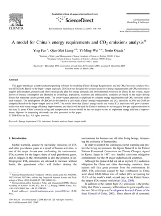
8. Y. Fan et al. / Environmental Modelling Software 22 (2007) 378e393 385
Table 4 Table 6
Forecast of China’s population (in billions) Forecast of ratio of renewable energy over primary energy (%)
Scenarios (organizations) 2010 2020 Ratios 2010 2020
High (CASS) 1.48 1.52 Hydro power 9.3 10.3
Low (UNEP) 1.39 1.45 Nuclear power 2.3 3.64
4.5.1. Total and per capita energy requirements and
most countries. In this scenario the urbanization rate will
related CO2 emissions
be 43.03% in 2010 and 50.14% in 2020.
Fig. 4 presents the results of energy requirements along
- Low scenario: China’s market-oriented reforms will not
with CO2 emissions in the model scenarios. In 2010, the total
significantly advance economic progress and the urbaniza-
energy requirement will be 1.57e1.84 billion tons of oil
tion process will still be constrained by the system as in
equivalent (toe), and the corresponding CO2 emissions will
the past 20 years. The urbanization rate will be 42.24%
be 1.33e1.57 billon tC; in 2020, the total energy requirement
in 2010 and 48.25% in 2020.
will be 1.88e2.64 billion toe, and corresponding CO2 emis-
sions will be 1.54e2.17 billion tC.
An analysis of the forecast results for these scenarios shows
4.2.4. Technology scenarios the followings.
4.2.4.1. Technology improvement matrix. Table 5 presents the 4.5.1.1. Energy efficiency plays an important role in the control
three sets of technology improvement scenarios. of energy consumption and related CO2 emissions. Scenario
A1 is one of the two scenarios with the highest level of energy
4.2.4.2. Ratio of renewable energy over primary energy. This needs and CO2 emissions. According to the scenario construc-
study utilizes the forecasts of the Academy of Macroeconomic tion, economic growth and urbanization advancement in this
Research Workgroup of the State Development Planning scenario are the lowest of all, which means the main driver
Commission (1999a) (Table 6). of energy consumption for final demand is the lowest. But
the improvement speed of energy efficiency in this scenario
is also the lowest; and thus the terminal energy requirement
4.3. Data and related CO2 emissions in this scenario are higher than
those in other scenarios.
Table 7 describes the data sources for the study. On the other hand, economic growth and urbanization ad-
vancement in scenario C2 occur at the same speed as in sce-
4.4. Model checking narios B and C1, and at a higher speed than in scenarios A1
and A2. Since improvement speed of energy efficiency is the
With the data from 1997, we checked our model for the highest in this scenario, the terminal energy requirement and
period 1998e2003, as shown in Fig. 3. Generally, the simula- related CO2 emissions in this scenario are lower than in other
tion results are close to the actual statistical data, with the scenarios except scenario A2.
largest relative error 11.19%, the smallest relative error Through this analysis it is clear that energy efficiency
0.90%, and the average relative error 2.21%. improvement plays an important role in the control of energy
Table 7
4.5. Simulation results and policy implication Data sources
Variable Source
In this section, the results of energy requirements and re- (matrix)
lated CO2 emissions in each scenario for 2010 and 2020 are Ac, Yc, Tu , c
Inputeoutput table of China (Department of National Accounts,
discussed. Tr , qf a
c
National Bureau of Statistics, P.R. China, 1997)
3fu , 3fr A modification of Hubacek and Sun (2001),
see Appendix B
Table 5 Lc , Lc , Pc , hc China Statistical Yearbook (National Bureau of Statistics, P.R.
u r
Technology scenarios China, 1998)
Cc, Wc Combining the data in energy balance tables
Scenario Description
1997 with the corresponding data in
Low Energy efficiency achieves a 5% less improvement than inputeoutput table of China (Department of National Accounts,
the medium case. National Bureau of Statistics, P.R. China, 1977; Department of
Medium The improvement of energy efficiency achieves the goal Industrial and Transportation Statistics, National Bureau of
of the National Energy-Saving Layout (Academy of Statistics, P.R. China, 2001)
Macroeconomic Research, State Development Planning a
The ratio of the construction sector is zero in the yearbook of 1997. Here
Commission, 1999b, see Appendix A for a brief introduction).
this ratio is set to be 15% which is allocated for urban and rural household
High Energy efficiency achieves a 5% greater improvement than
consumption based on the ratio between urban and rural population (Hubacek
the medium case.
and Sun, 2001).

9. 386 Y. Fan et al. / Environmental Modelling Software 22 (2007) 378e393
1200.00
1100.00
1000.00
900.00
800.00
700.00
600.00
500.00
1997 1998 1999 2000 2001 2002 2003
simulation results 924.56 813.91 881.53 893.26 955.89 1106.54 1138.06
statistic data 924.56 887.72 873.66 874.85 905.85 995.20 1126.66
simulation results statistic data
Fig. 3. Energy demand (requirements) for 1998e2003 (million toe).
consumption and related CO2 emissions. Great efforts should C2. The result is that energy consumption along with CO2
be taken to improve energy efficiency in final demand sectors, emissions in this scenario for the two final years are both lower
to enhance energy conversion efficiency, and to gradually than in scenario C2. It is obvious that the low energy con-
create a lower energy consumed product system and a life sumption and low CO2 emissions in scenario A2 is obtained
system. at the cost of a low economic growth rate.
The above results show that total energy requirements and
4.5.1.2. Population has a significant impact on energy require- CO2 emissions increase rapidly in all scenarios. As for per
ments along with CO2 emissions. Scenario C1 is the ‘‘high capita results, Fig. 5 compares per capita CO2 emissions in
population’’ scenario in which the energy requirements and re- each scenario with the world average in 2003. It appears that
lated CO2 emissions will be second place in 2010, and rise to in 2010, per capita CO2 emissions in scenario A1 are slightly
first place in 2020. So even with the development of technol- higher than the world average in 2003. Per capita CO2 emis-
ogy, energy requirements along with CO2 emissions will still sions in all the scenarios will rise until 2020 by more than
increase rapidly if planners and policymakers fail to control the world rate in 2003.
population at the same time.
4.5.2. Energy structure and CO2 emissions by energy type
4.5.1.3. Energy efficiency is highly related to economic The forecast of energy structure and CO2 emissions by
growth. Energy efficiency in scenario A2 improves slower energy type are shown in Figs. 6 and 7, respectively.
than that in scenario C2, but economic growth and urbaniza- Variations of energy structures in all scenarios are similar in
tion rates are also slower in this scenario than in scenario general. The proportion of coal decreases, but still occupies
3.00
Energy requirements (billion toe) CO2 emissions (billion tC)
2.50
2.00
1.50
1.00
0.50
0.00
1997 2010 2020 1997 2010 2020
A1 0.94 1.84 2.50 0.87 1.57 2.06
A2 0.94 1.57 1.88 0.87 1.33 1.54
B 0.94 1.67 2.52 0.87 1.42 2.08
C1 0.94 1.78 2.64 0.87 1.51 2.17
C2 0.94 1.59 2.31 0.87 1.35 1.90
Fig. 4. Results of energy requirements and related CO2 emissions in assigned scenarios.

10. Y. Fan et al. / Environmental Modelling Software 22 (2007) 378e393 387
1.5
Per capita CO2 emissions (tC/capita)
1.4
1.3
1.2
1.1
1
0.9
0.8
0.7
0.6
0.5
1997 2010 2020
ScenarioA1 ScenarioA2 ScenarioB
ScenarioC1 ScenarioC2 World Average 2003
Fig. 5. China’s per capita CO2 emissions in 2010 and 2020 vs. world average level in 2003.
the principal usage; the proportions of oil and natural gas rises, In the two final years, both the lowest energy intensity and
but the share of natural gas use is still low. CO2 intensity appear in scenario C2, and both the highest en-
As shown in Table 1, the potential emissions factor of coal ergy intensity and CO2 intensity appear in scenario A1.
is much larger than that of oil and natural gas. Thus, generally, In general, energy intensity and CO2 intensity are declin-
the energy structure tends to impact more significant on CO2 ing. CO2 intensity is declining faster than energy intensity be-
emissions control. But since coal still dominates the energy cause CO2/TPEC, another factor determining CO2 intensity, is
structure, CO2 emissions by coal is the largest emissions factor also declining.
in the future two years (see Fig. 7). So it appears that the But in all the scenarios the decline of CO2/TPEC is slow.
potential to control CO2 emissions by adjusting the energy This implies that in two final years the coal-dominated energy
structure during this period is limited. structure is changing very little. CO2/TPEC determines the
variation speed of CO2 intensity. The slow declining speed
4.5.3. Energy intensity, CO2 intensity and CO2/TPEC of CO2/TPEC to a great extent limits the decline of CO2 emis-
In 2010, energy intensity will be 0.79e1.023 toe/104 Yuan, sions in this period.
CO2 intensity will be 0.671e0.87 tC/104 Yuan, and CO2/
TPEC will be about 0.85 tC/toe. In 2020, energy intensity 4.5.4. Relationship between CO2 emissions
will be 0.604e0.864 toe/104 Yuan, CO2 intensity will be and driving factors
0.497e0.711 tC/104 Yuan, and CO2/TPEC will be about According the definition of CO2 emissions, the following
0.823 tC/toe. decomposition was performed to assess the impacts of major
Table 8 shows the change rate of energy intensity and CO2 driving forces on CO2 emissions:
intensity in 2010 vs. 1997, and 2020 vs. 2010.
CO2 emissions ¼ CO2 intensity  GDP
2020 C2
¼ CO2 =TPEC  energy intensity  GDP
2020 C1
2020 B 2020 C2
2020 A2 2020 C1
2020 B
2020 A1
2020 A2
2010 C2
2020 A1
2010 C1
2010 C2
2010 B 2010 C1
2010 A2 2010 B
2010 A2
2010 A1
2010 A1
Base year
Base year
0% 20% 40% 60% 80% 100% 0% 20% 40% 60% 80% 100%
Coal Oil Natural Gas Other Coal Oil Natural Gas
Fig. 6. Energy structure in constructed scenarios (%). Fig. 7. CO2 emissions by energy type in constructed scenarios (%).

11. 388 Y. Fan et al. / Environmental Modelling Software 22 (2007) 378e393
Table 8 driving forces of the ratio of fossil energy over primary energy
Change rate of energy intensity and CO2 intensity and that of CO2/TFES are quite small.
Scenarios 2010 vs. 1997 2020 vs. 2010 In all the scenarios, the forward driving effect of per capita
Energy intensity CO2 intensity Energy intensity CO2 intensity GDP growth is much larger than the backward driving effects
A1 0.82 0.76 0.84 0.82 of other factors, which can explain why CO2 emissions are
A2 0.70 0.65 0.75 0.72 growing so fast.
B 0.67 0.62 0.79 0.77 Between 2010 and 2020, the backward driving effect of en-
C1 0.71 0.66 0.78 0.75 ergy intensity is smaller than between 1997 and 2010, which
C2 0.64 0.59 0.76 0.74
shows that further technology enhancements will become
more difficult. Therefore, on the one hand, certain policies
should be devised to promote changes in energy structure
¼ CO2 =TFEC so as to effectively make use of the backward driving effect
 the ratio of fossil energy over primary energy of the ratio of fossil energy over primary energy and that of
CO2/TFES. On the other hand, changing energy structure
 energy intensity  per capita GDP  population
would be a long-term task, the effect of which is not quite
likely to be seen before 2020 (Zhou and Yukio, 1996), so
where, CO2/TFEC presents CO2 emissions from the total fos- the coal-dominated energy structure is not expected to change
sil energy consumption. too much in the near future, the decline of energy intensity is
The variation of CO2 emissions and that of each driving limited; correspondingly the decline of CO2 intensity is also
force are calculated, respectively, as presented in Fig. 8. limited. Moreover, during this period China’s economy will
The decomposition implies that, in the absence of extra still grow at a relatively high speed, so the potential for CO2
energy or environmental policies, among all the driving mitigation is limited.
factors, per capita GDP plays the most important role, energy
intensity comes in second, and population, third, while the 4.5.5. Sector energy requirements and CO2 emissions
Figs. 9 and 10 show the results of sector and residential en-
ergy requirements and CO2 emissions, respectively.
C2
Variations in all the scenarios are similar. The energy need
in manufacturing sector is declining, which shows the impact
C1
of the accelerated development of service and transportation
caused by accelerated urbanization. But due to the govern-
2010-2020
B ment’s objective ‘‘to achieve industrialization by 2020,’’ the
scale of manufacturing will still expand. The energy require-
A2 ments and CO2 emissions of this sector will still take the larg-
est share, followed by the transportation sector.
A1 The share of energy for the agriculture sector first increases
and then declines: the share in 2010 is larger than in 1997,
while the share in 2020 is smaller than in 2010, but is still
larger than in 1997. This phenomenon can be explained by
the two driving forces of opposite directions on agriculture en-
C2
ergy consumption, i.e., the continuous decrease in agricultural
energy usage in the industrial structure has a backward impact,
C1 while the continuous increase in the agricultural mechaniza-
tion level has a positive impact.
1997-2010 The shares of construction and commerce in total energy
B
consumption increase rapidly. The shares of transportation
A2 and the service industry in 2010 rise markedly from the
1997 level, while their shares in 2020 vary not much from
A1
those in 2010, they rise just a little.
0 0.5 1 1.5 2 2.5 3 4.5.6. Sector energy intensity and CO2 intensity
population Tables 9 and 10 present the results of sector energy inten-
per capita GDP sity and CO2 intensity, respectively.
energy intensity
In the two final years, the energy and CO2 intensities of the
ratio of fossil energy over primary energy
CO2/TFES
manufacturing and transportation sectors are evidently higher
CO2 emissions
than average.
For manufacturing, energy and CO2 intensities in scenario
Fig. 8. Relationships between CO2 emissions and driving factors. A1 are much higher than those in the other four scenarios.

12. Y. Fan et al. / Environmental Modelling Software 22 (2007) 378e393 389
100%
90%
80%
70%
60%
50%
40%
30%
20%
10%
0%
Base 2010 A1 2020 A1 2010 A2 2020 A2 2010 B 2020 B 2010 C1 2020 C1 2010 C2 2020 C2
year
Agriculture Manufacturing Construction Transportation
Commerce Service Residential
Fig. 9. Sector energy requirement in each scenario (%).
For transportation, in 2010, energy intensity in all scenarios is 4.6. Policy implications
quite close to that of manufacturing.
Manufacturing and transportation take the largest shares of Summarizing the above forecast results and analyses of the
energy and produce the largest amount of CO2 emissions, thus model, the following policy recommendations are proposed.
the energy and CO2 intensities of these two sectors will to
a great extent impact the speed of energy requirements and
CO2 emissions growth. These two sectors should be pivotal 4.6.1. Policies promoting changes in energy structure
in improving energy efficiency. should be devised to control the quickly increasing
Among all scenarios, scenario A1 is the worst path in terms CO2 emissions
of controlling the fast growth trends of energy requirements The above forecast results show that even in scenario C2,
and CO2 emissions. where technology advances the fastest, CO2 emissions
Energy and CO2 intensities in agriculture, construction, increase rapidly. Moreover, the increase of per capita emis-
commerce and the non-material sectors remain lower than sions will quite possibly reach or exceed the worldwide aver-
the sector average. The intensities of the construction sector age within 20 years. The results also show that with time
are the lowest in the two final years, but tend to rise rapidly. goes on further enhancements in energy-saving technology
As shown above, the shares of construction and commerce will become more and more difficult. Therefore, it is desir-
in total energy consumption increase rapidly, there could be able to establish energy and environmental policies in favor
an induced reduction in CO2 emissions. Therefore great efforts of cleaner energies as early as possible to accelerate the
should be taken to maintain the low energy and CO2 intensities changes in energy structure and to support sustainable eco-
in these sectors. nomic development.
100%
80%
60%
40%
20%
0%
Base 2010 A1 2020 A1 2010 A2 2020 A2 2010 B 2020 B 2010 C1 2020 C1 2010 C2 2020 C2
year
Agriculture Construction Commerce Residential
Manufacturing Transportation Service
Fig. 10. Sector CO2 emissions in each scenario (%).

13. 390 Y. Fan et al. / Environmental Modelling Software 22 (2007) 378e393
Table 9 than that of oil and natural gas in most cases (He et al.,
Energy intensity for each sector (toe/104 Yuan) 1995), the decline of energy intensity will likely be limited
Sector 2010 2020 over the next 15 years. At the same time, the high cardinal
A1 A2 BAU C1 C2 A1 A2 BAU C1 C2 number of coal, to a great extent, will likely limit the decrease
Agriculture 0.35 0.31 0.29 0.31 0.28 0.35 0.27 0.27 0.28 0.25 of CO2 emissions by total fossil fuel consumption, which can
Manufacturing 1.86 1.58 1.52 1.61 1.44 1.47 1.11 1.17 1.23 1.07 still cover the majority of total primary energy consumption.
Construction 0.18 0.15 0.14 0.15 0.13 0.23 0.16 0.17 0.17 0.15 Consequently CO2 intensity will likely not drop considerably
Transportation 1.95 1.55 1.49 1.58 1.41 1.88 1.26 1.29 1.35 1.17 fast in the next 20 years.
Commerce 0.30 0.26 0.25 0.27 0.24 0.26 0.21 0.21 0.22 0.20
Service 0.29 0.26 0.25 0.26 0.24 0.26 0.21 0.21 0.22 0.20
Sector average 1.02 0.87 0.83 0.89 0.79 0.86 0.65 0.66 0.69 0.60 5. Discussion and perspectives
The application shows that CErCmA provides an effective
4.6.2. Effective policies should be developed and
tool for assessing energy requirements along with CO2 emis-
implemented to encourage governmental agencies
sions in China. The combination of scenario analysis and the
and corporations to increase energy efficiency
inputeoutput model provides not only a thorough, integrated
The model results clearly show that in all scenarios energy
analysis, but also a means to explicitly assess the impact of
intensity has an obvious backward driving effect on CO2 emis-
each driving force.
sions, second only to the forward driving effect of per capita
Further work is needed to address the followings in order to
GDP. What’s more, efforts to change China’s coal-dominated improve our model.
energy structure will take a long term to take effect, thus en-
ergy efficiency improvement will still play a pivotal role in
5.1. The limitation of the static IeO model
CO2 mitigation.
The manufacturing and transportation sectors consume the
So far, the methodology of the dynamic IeO model is
major share of energy in China, and their energy intensities are
still being developed. For our current system we chose the
very high, much higher than the sector average. Model results
classical static IeO model. However, a complete static
show that their share of emissions is decreasing but will main-
approach would fail to identify the structural changes. To
tain the main part of total CO2 emissions in recent 20 years.
address this problem, we applied an adjustment to the base
The high CO2 intensity of manufacturing is determined by
year direct requirement matrix Ac by using the RAS approach
its high energy intensity. Therefore, certain policies must be
to obtain a possible structural change in this paper. In this
continuously implemented to decrease the manufacturing sec-
way, we could simulate the structural changes during the
tor’s energy intensity, such as accelerating the adjustment of
time horizon of our study.
the industrial and product structures within the manufacturing
Nevertheless, the RAS approach has some weakness,
sectors to improve manufacturing energy efficiency.
primarily its economic assumptions: the sector consistency
The shares of construction and commerce in total energy
of substitution and manufacturing impacts is not satisfied in
consumption increase rapidly, thus there is an induced reduction
many cases. One way to improve the RAS approach may be
in CO2 emissions because of the low CO2 intensities of these
to combine it with a case study of the key coefficients in a di-
two sectors. Therefore particular attentions should also be
rect requirement matrix. Today, a great deal of attention is be-
paid to the energy efficiency improvements in these two sectors.
ing focused on improving this approach. Accordingly, in the
future, we plan to trace the development of the RAS approach
4.6.3. The potential for CO2 mitigation in China is limited in and other possibly more effective adjustment approaches to
the next 20 years, and thus decision making should be improve the precision of the current system.
based on this key point
From today until the 2020, China’s GDP is expected to 5.2. Technology scenario base
maintain a high growth rate. While the special coal-dominated
energy structure is not expected to change much in the near Because of data availability limitations, the technology
future, and because the efficiency of coal is much lower scenarios in the current version were attained by adjusting cur-
Table 10 rent energy layouts. This kind of data source would, to some
Sector CO2 intensity (tC/104Yuan) extent, weaken the plausibility of the technology scenarios
Sector 2010 2020 and limit the assessment of the impact of technology in terms
of depth. In future studies, researchers should try to improve
A1 A2 BAU C1 C2 A1 A2 BAU C1 C2
the technology scenario base.
Agriculture 0.29 0.25 0.24 0.25 0.23 0.27 0.21 0.21 0.22 0.20
Manufacturing 1.61 1.37 1.32 1.40 1.25 1.24 0.94 0.99 1.04 0.91
Construction 0.14 0.12 0.11 0.12 0.11 0.18 0.13 0.13 0.14 0.12 5.3. Carbon tax analysis: quantifying policy
Transportation 1.50 1.20 1.15 1.22 1.09 1.41 0.95 0.97 1.01 0.88 recommendations
Commerce 0.25 0.21 0.21 0.22 0.20 0.21 0.17 0.17 0.18 0.16
Service 0.22 0.20 0.19 0.20 0.18 0.20 0.16 0.16 0.17 0.15 Quantifying the feedback of certain policies could
Sector average 0.87 0.74 0.71 0.75 0.67 0.71 0.53 0.54 0.57 0.50
enable us to test the possible executive effects of the

14. Y. Fan et al. / Environmental Modelling Software 22 (2007) 378e393 391
policies. Carrying out a carbon tax analysis can be a possible will increase by 10.5%, from 45% in 1995 to 55.5%
application if the carbon tax can be incorporated into the in 2010.
model.
(4) Transportation industry.
5.4. Models on the regional level Energy efficiency in 2010 will be a little higher than that
in 1995.
Current version only includes models on the national
level. However, social and economic factors, such as (5) Household energy consumption.
population intensity and income levels, as well as energy effi-
ciency significantly differ among regions in China. Modeling en- In 2010, urban household energy efficiency is hopefully to
ergy requirements and CO2 emissions on a regional level would reach 50% of the level of developed countries in early
be of great help to energy and environment policy making. 1990s; rural household efficiency will rise from 25% in
1995 to 45%.
(6) Other industries.
Acknowledgements
In 2010, energy efficiency is hopefully to reach the level
The authors gratefully acknowledge the financial support
of developed countries in early 1990s, i.e., rise 5 to 10%
from the National Natural Science Foundation of China
from the level of 1995.
(NSFC) under the grants Nos.70425001, 70573104 and
70371064, the Key Projects from the Ministry of Science and
Technology of China (grants 2001-BA608B-15, 2001-BA605-
01), Harvard University Committee on Environment China Pro- Appendix B
ject. Ying Fan would like to thank Prof. Tom Lyons, Prof. Yong-
Income elasticity of various sectors
miao Hong and Ms. Deborah Campbell at Cornell University for
Sectors 1992e2005 2005e2025
their valuable comments and kind help. Yi-Ming Wei truly ap-
preciates the supports from Prof. Michael B. McElroy and Mr. Rural Urban Rural Urban
Chris P. Nielsen at Harvard University. We also would like to Agriculture 0.561 0.767 0.509 0.743
thank Prof. A. J. Jakeman and the other four anonymous referees Manufacturing 1.100 1.100 1.100 1.100
Construction 1.100 1.100 1.100 1.100
for their helpful comments on the earlier draft of our paper ac-
Transportation 1.200 1.200 1.200 1.200
cording to which we improved the content. Commerce 1.200 1.200 1.200 1.200
Services 1.200 1.200 1.200 1.200
A modification of Hubacek and Sun (2001).
Appendix A. A brief introduction of the National
Energy-Saving Layout
References
The Group of the Academy of Macroeconomic Research of
the State Development Planning Commission figured out the po- Bach, S., Kohlhaas, M., Meyer, B., Praetorius, B., Welsch, H., 2002. The
tential of energy efficiency improvement in sectoral final energy effects of environmental fiscal reform in Germany: a simulation study.
Energy Policy 30, 803e811.
consumption through adopting various techniques and mea-
Ball, M., Calaminus, B., Kerdoncuff, P., Rentz, O., 2005. Techno-economic da-
sures. (Workgroup of the Academy of Macroeconomic Re- tabases in the context of integrated assessment modelling. Environmental
search of the State Development Planning Commission, 1999b). Modelling Software 20, 1189e1193.
Chen, W.Y., 2005. The costs of mitigating carbon emissions in China:
(1) Iron and steel industry. findings from China MARKAL-MACRO modeling. Energy Policy 33,
885e896.
Christodoulakis, N.M., Kalyvitis, S.C., Lalas, D.P., Pesmajoglou, S., 2000.
Energy efficiency can rise by 12%, from 46% in 1995 to Forecasting energy consumption and energy related CO2 emissions in
58% in 2010, a bit higher than that of industrialized coun- Greece: an evaluation of the consequences of the Community Support
try in early 1970s. Framework II and natural gas penetration. Energy Economics 22,
395e422.
(2) Materials industry. Clinch, J.P., Healy, J.D., King, C., 2001. Modelling improvements in
domestic energy efficiency. Environmental Modelling Software 16,
Energy use per unit output will decrease. Annually energy 87e106.
Crompton, P., Wu, Y.R., 2005. Energy consumption in China: past trends and
save rate will be 1.5%. Energy efficiency will increase by
future directions. Energy Economics 27, 195e208.
10%, from 40% in 1995 to 50% in 2010. Cruz, Luis M.G., 2002. Energyeenvironmenteeconomy interactions: an
inputeoutput approach applied to the Portuguese Case. Paper for the 7th
(3) Building materials industry.
Biennial Conference of the International Society for Ecological Econom-
ics, ‘‘Environment and Development: Globalisation the Challenges
Energy use per unit output will decrease. Annually for Local International Governance, ’’ Sousse (Tunisia), 6e9 March
energy-saving rate will be 1.4%. Energy efficiency 2002.