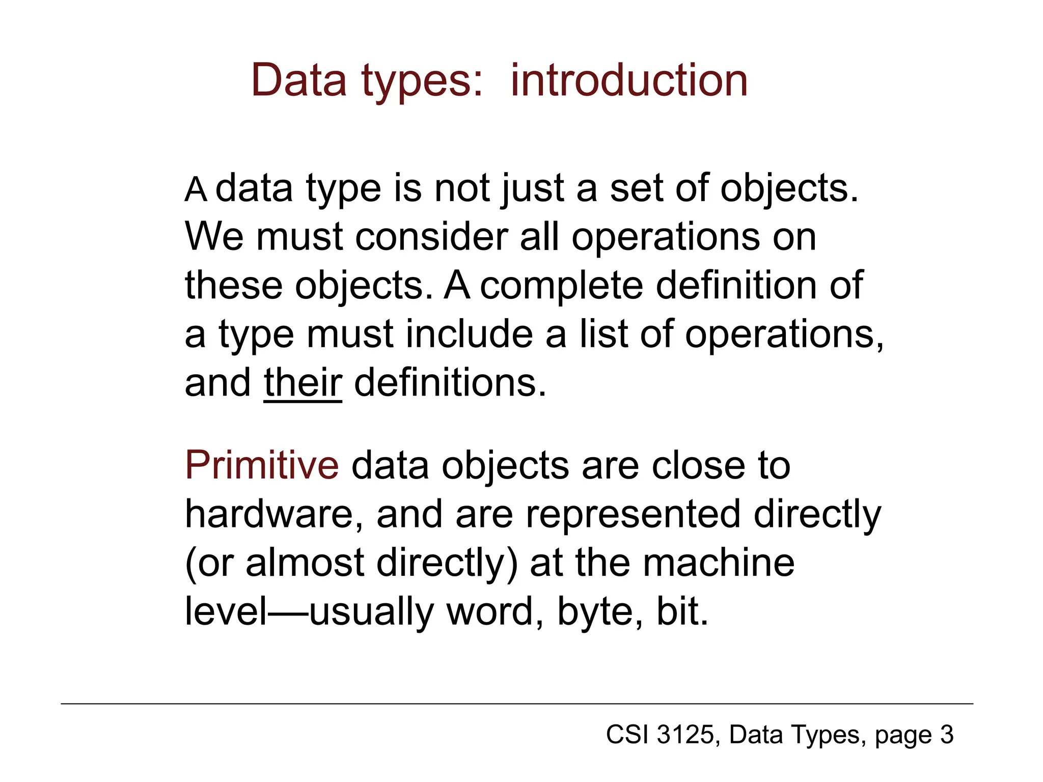
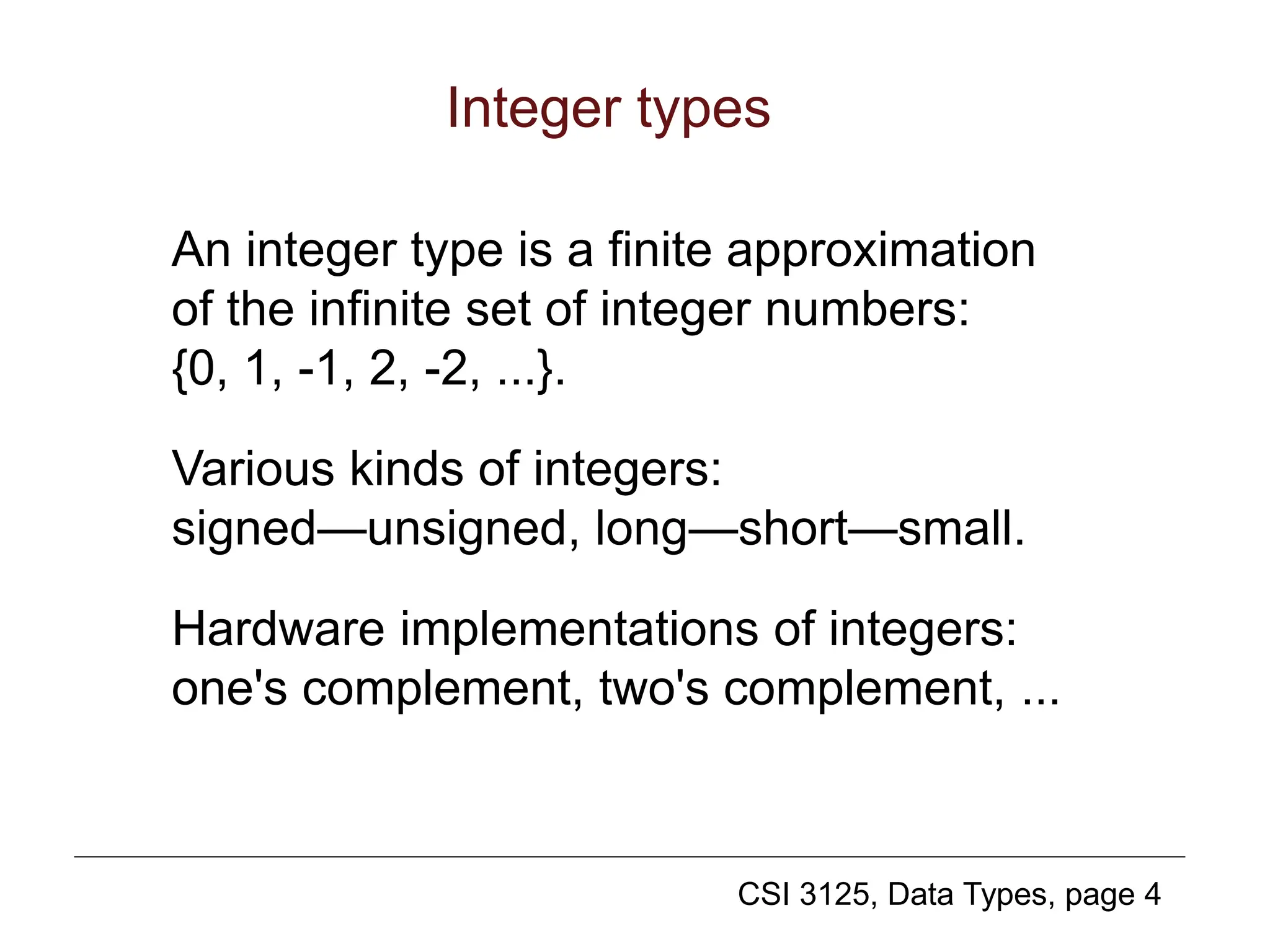
The document outlines various data types in programming, including primitive types like integers, floating-point numbers, booleans, and characters, as well as structured types such as strings, enumerated types, arrays, and records. It explains the characteristics and operations associated with each type, detailing how they are implemented in different programming languages. Additionally, the document discusses pointers as a means of dynamically managing data structures and their operations.
![CSI 3125, Data Types, page 15
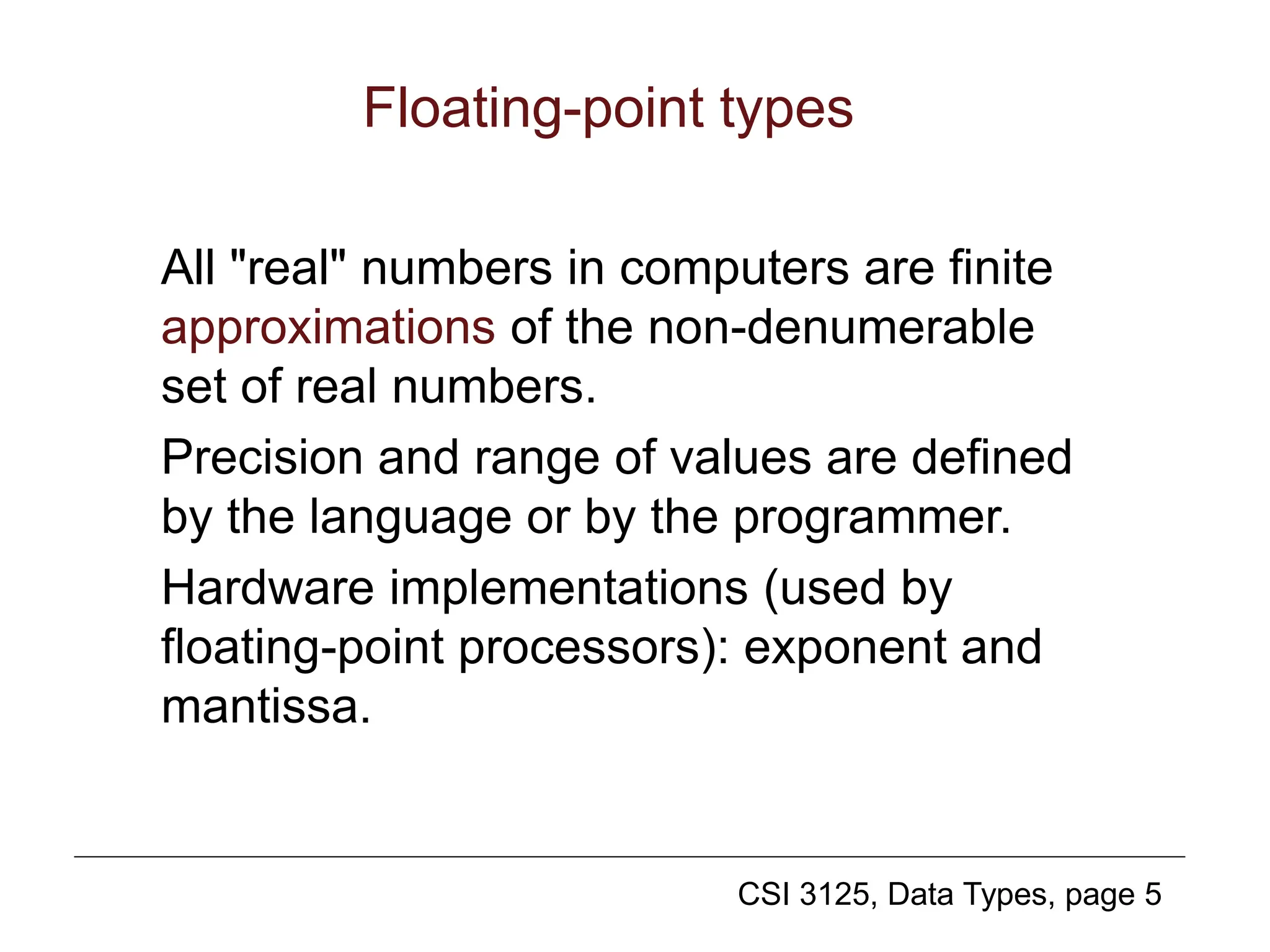
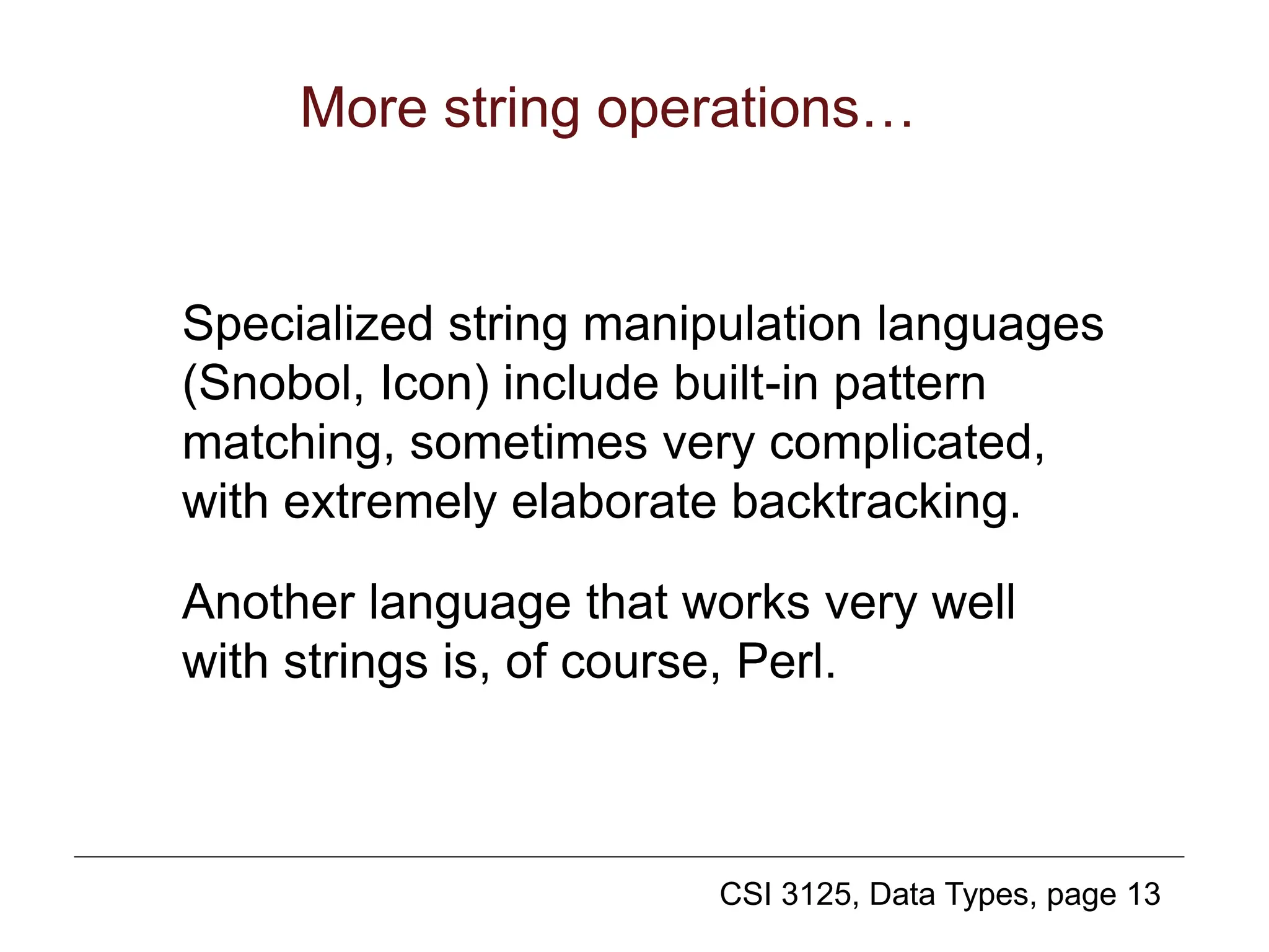
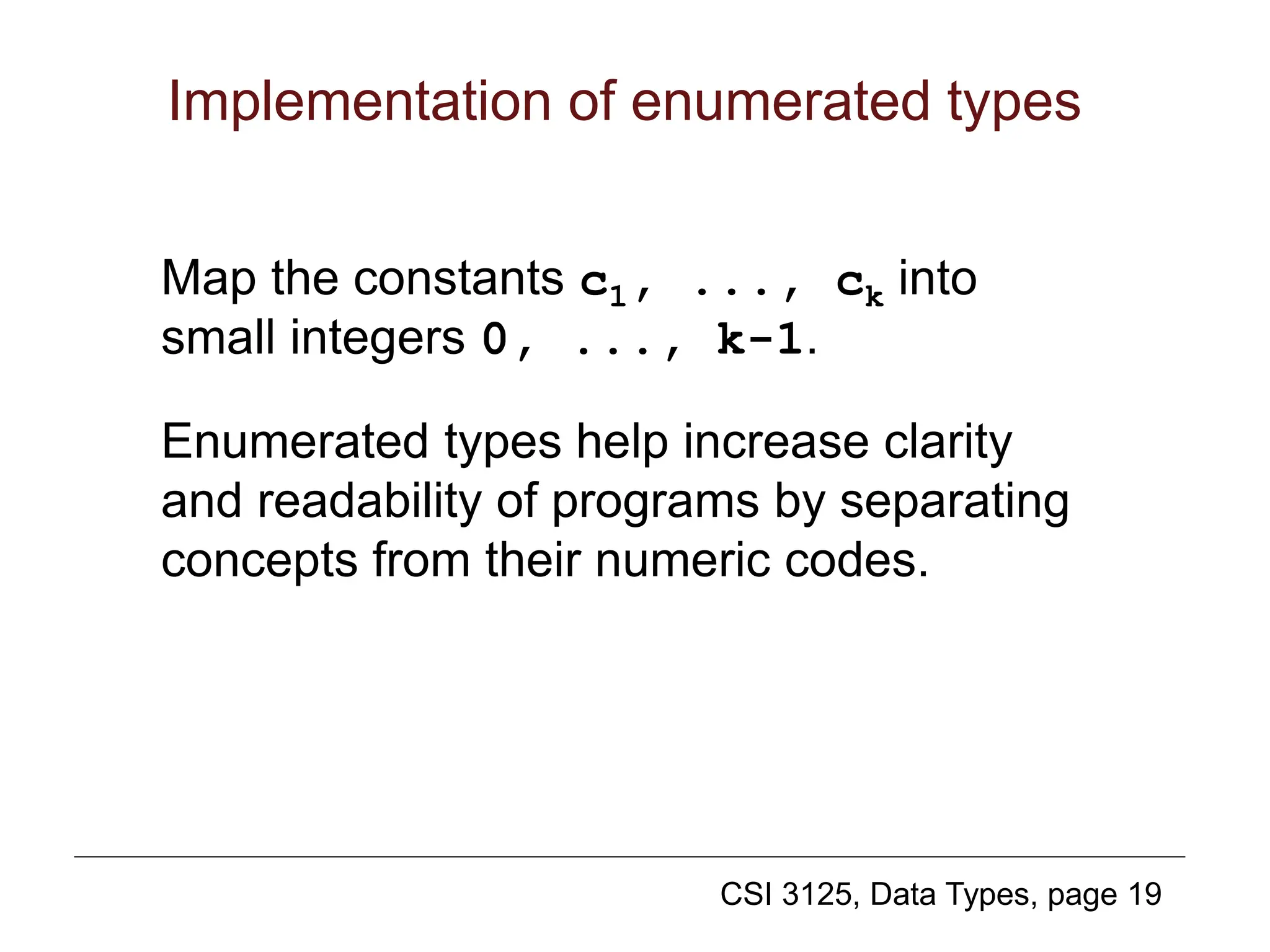
Enumerated types
Also called: user-defined ordinal types
[read Section 6.4]
We can declare a list of symbolic constants that are
to be treated literally, just like in Prolog or Scheme.
We also specify the implicit ordering of those newly
introduced symbolic constants. In Pascal:
type day =
(mo, tu, we, th, fr, sa, su);
Here, we have mo < tu < we < th < fr < sa < su.](https://image.slidesharecdn.com/09datatypes-240420100358-35269b6b/75/09_java_DataTypesand-associated-class-ppt-15-2048.jpg)

![CSI 3125, Data Types, page 21
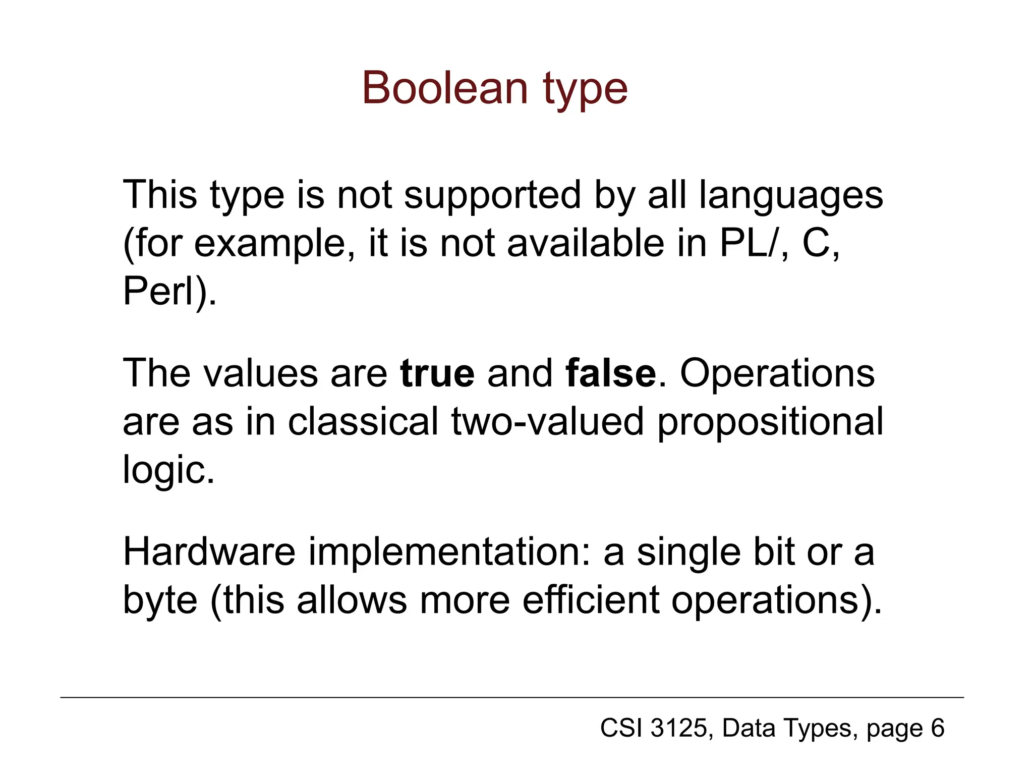
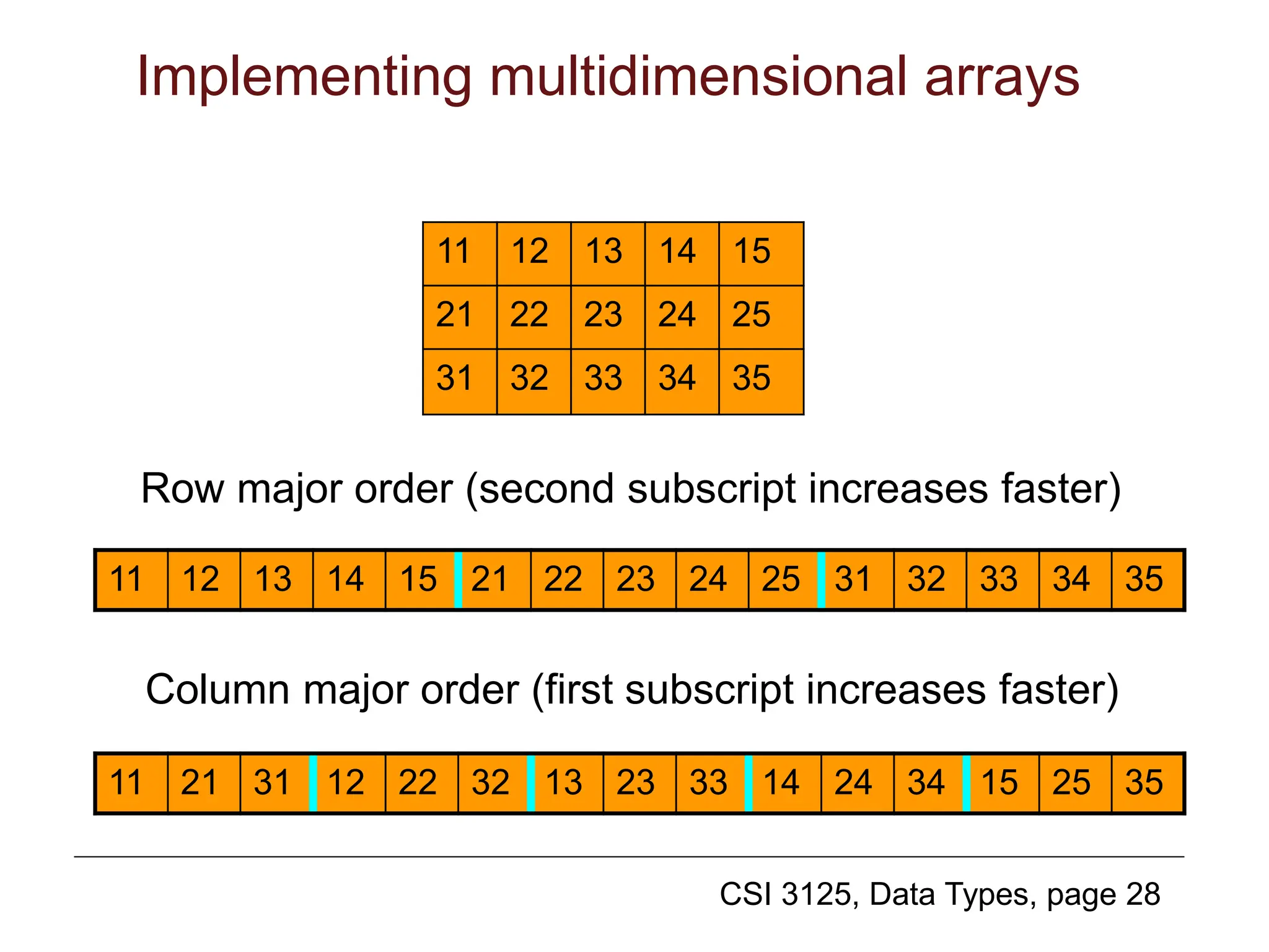
Multidimensional arrays
Multidimensional arrays can be defined in two
ways (for simplicity, we show only dimension 2):
index_type1 index_type2 component_type
This corresponds to references such as A[I,J].
Algol, Pascal, Ada work like this.
index_type1 (index_type2 component_type)
This corresponds to references such as A[I][J].
Java works like this.
Perl sticks to one dimension](https://image.slidesharecdn.com/09datatypes-240420100358-35269b6b/75/09_java_DataTypesand-associated-class-ppt-21-2048.jpg)
![CSI 3125, Data Types, page 22
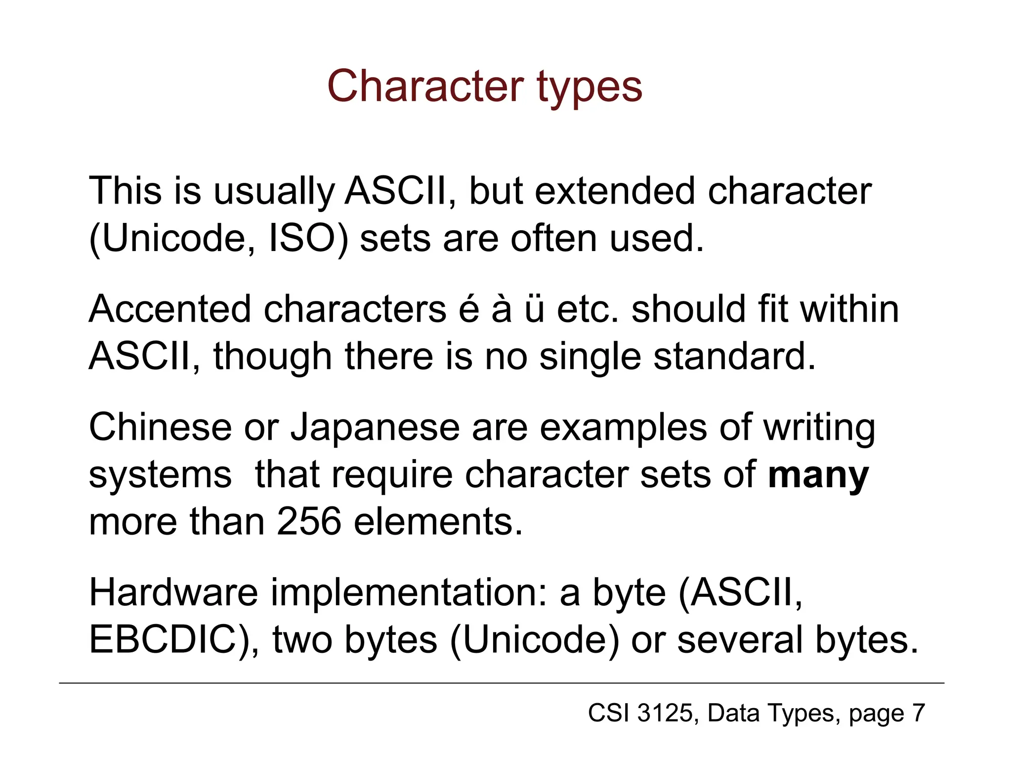
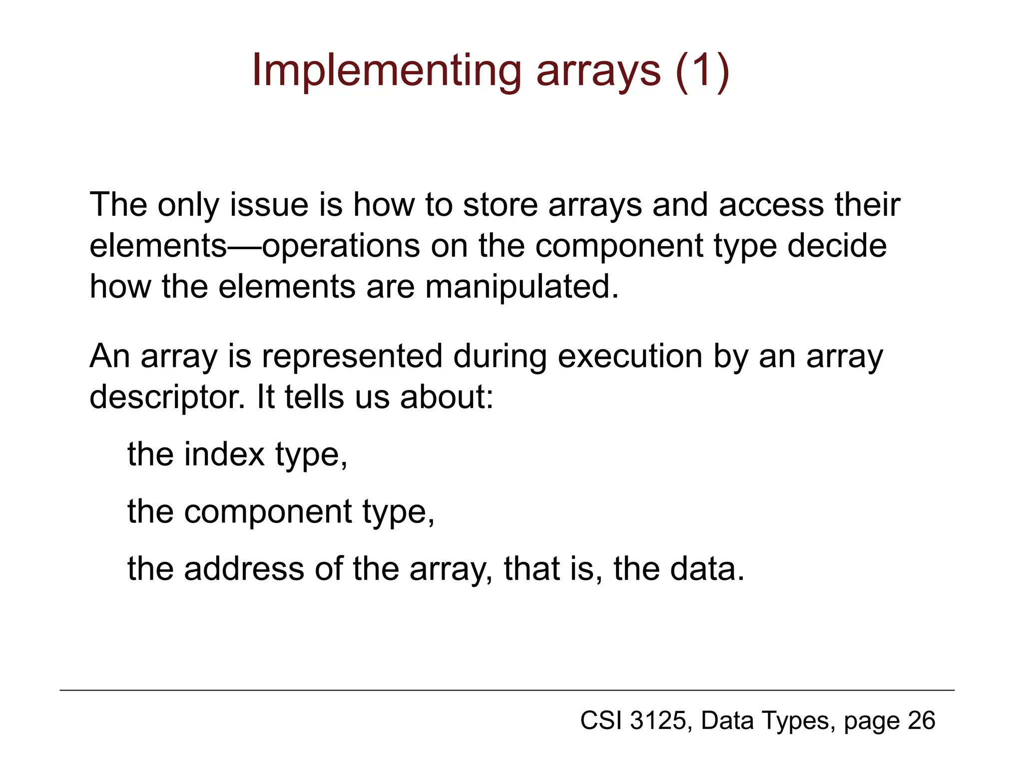
Operations on arrays (1)
select an element (get or change its value):
A[J]
select a slice of an array:
(read the textbook, Section 6.5.7)
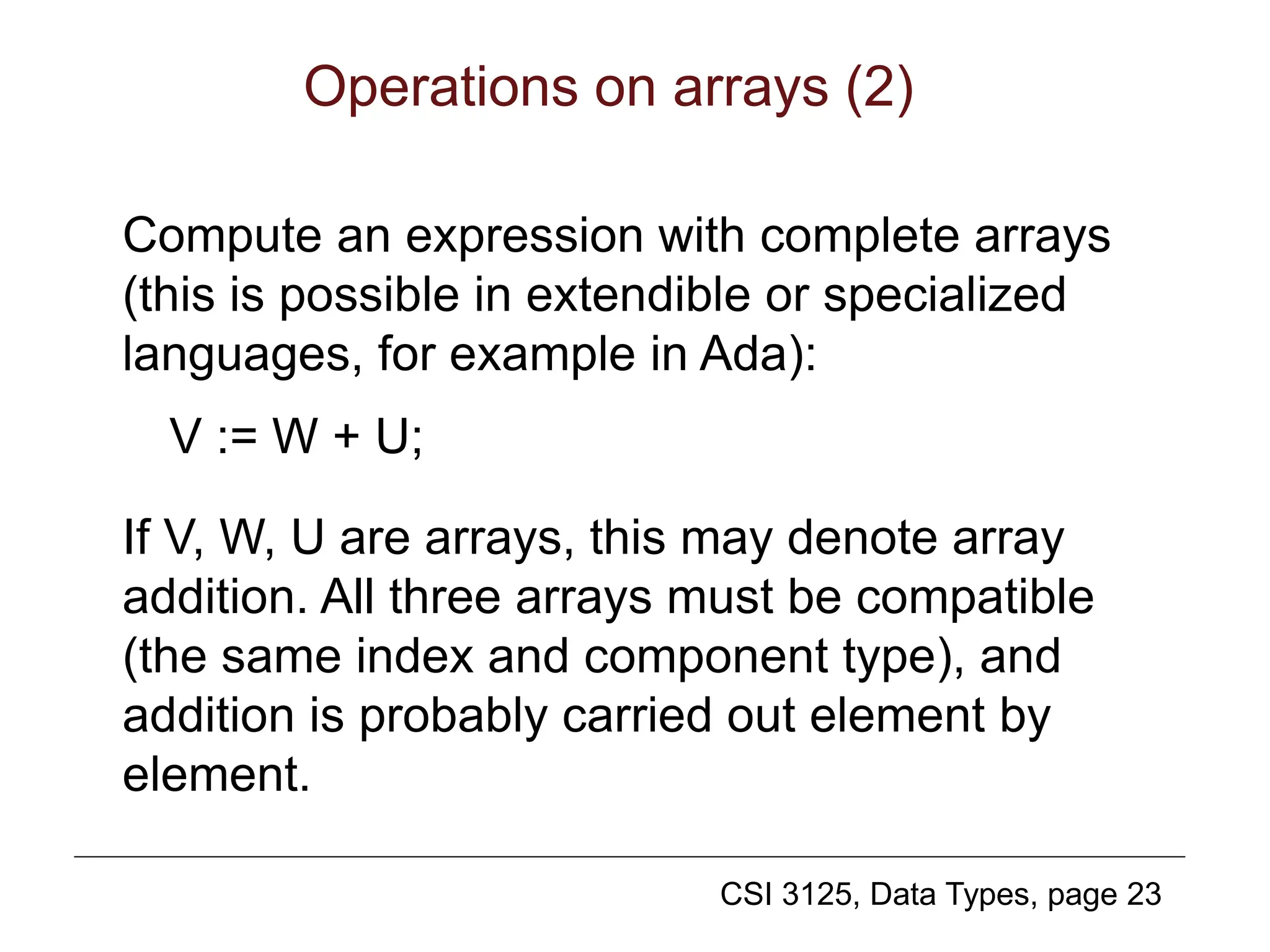
assign a complete array to a complete array:
A := B;
There is an implicit loop here.](https://image.slidesharecdn.com/09datatypes-240420100358-35269b6b/75/09_java_DataTypesand-associated-class-ppt-22-2048.jpg)
![CSI 3125, Data Types, page 25
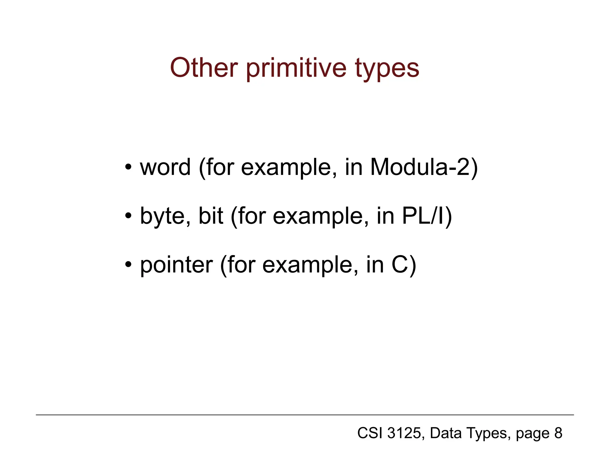
Array-type constants and initialization
Many languages allow initialization of arrays to be
specified together with declarations:
C int vector [] = {10,20,30};
Ada vector: array(0..2)
of integer := (10,20,30);
Array constants in Ada
temp is array(mo..su)of -40..40;
T: temp;
T := (15,12,18,22,22,30,22);
T := (mo=>15, we=>18, tu=>12,
sa=>30, others=>22);
T := (15,12,18, sa=>30, others=>22);](https://image.slidesharecdn.com/09datatypes-240420100358-35269b6b/75/09_java_DataTypesand-associated-class-ppt-25-2048.jpg)
![CSI 3125, Data Types, page 29
Suppose that we have this array:
A: array [LOW1..HIGH1,
LOW2..HIGH2] of ELT;
where the size of each entity of type ELT is
SIZE.
This calculation is done for row-major
(calculations for column-major are quite
similar). We need the base—for example,
the address LOC of A[LOW1, LOW2].
Implementing multidimensional arrays (2)](https://image.slidesharecdn.com/09datatypes-240420100358-35269b6b/75/09_java_DataTypesand-associated-class-ppt-29-2048.jpg)
![CSI 3125, Data Types, page 30
We can calculate the address of A[I,J] in the
row-major order, given the base.
Let the length of each row in the array be:
ROWLENGTH = HIGH2 - LOW2 + 1
The address of A[I,J] is:
(I - LOW1) * ROWLENGTH * SIZE +
(J - LOW2) * SIZE + LOC
Implementing multidimensional arrays (3)](https://image.slidesharecdn.com/09datatypes-240420100358-35269b6b/75/09_java_DataTypesand-associated-class-ppt-30-2048.jpg)
![CSI 3125, Data Types, page 31
Here is an example.
VEC: array [1..10, 5..24] of integer;
The length of each row in the array is:
ROWLENGTH = 24 - 5 + 1 = 20
Let the base address be 1000, and let the size of
an integer be 4.
The address of VEC[i,j] is:
(i - 1) * 20 * 4 + (j - 5) * 4 + 1000
For example, VEC[7,16] is located in 4 bytes at
1524 = (7 - 1) * 20 * 4 +
(16 - 5) * 4 + 1000
Implementing multidimensional arrays (4)](https://image.slidesharecdn.com/09datatypes-240420100358-35269b6b/75/09_java_DataTypesand-associated-class-ppt-31-2048.jpg)
![CSI 3125, Data Types, page 32
Languages without arrays
A final word on arrays: they are not supported
by standard Prolog and pure Scheme. An array
can be simulated by a list, which is the basic
data structure in Scheme and a very important
data structure in Prolog.
Assume that the index type is always 1..N.
Treat a list of N elements:
[x1, x2, ..., xN] (Prolog)
(x1 x2 ... xN) (Scheme)
as the (structured) value of an array](https://image.slidesharecdn.com/09datatypes-240420100358-35269b6b/75/09_java_DataTypesand-associated-class-ppt-32-2048.jpg)
![CSI 3125, Data Types, page 40
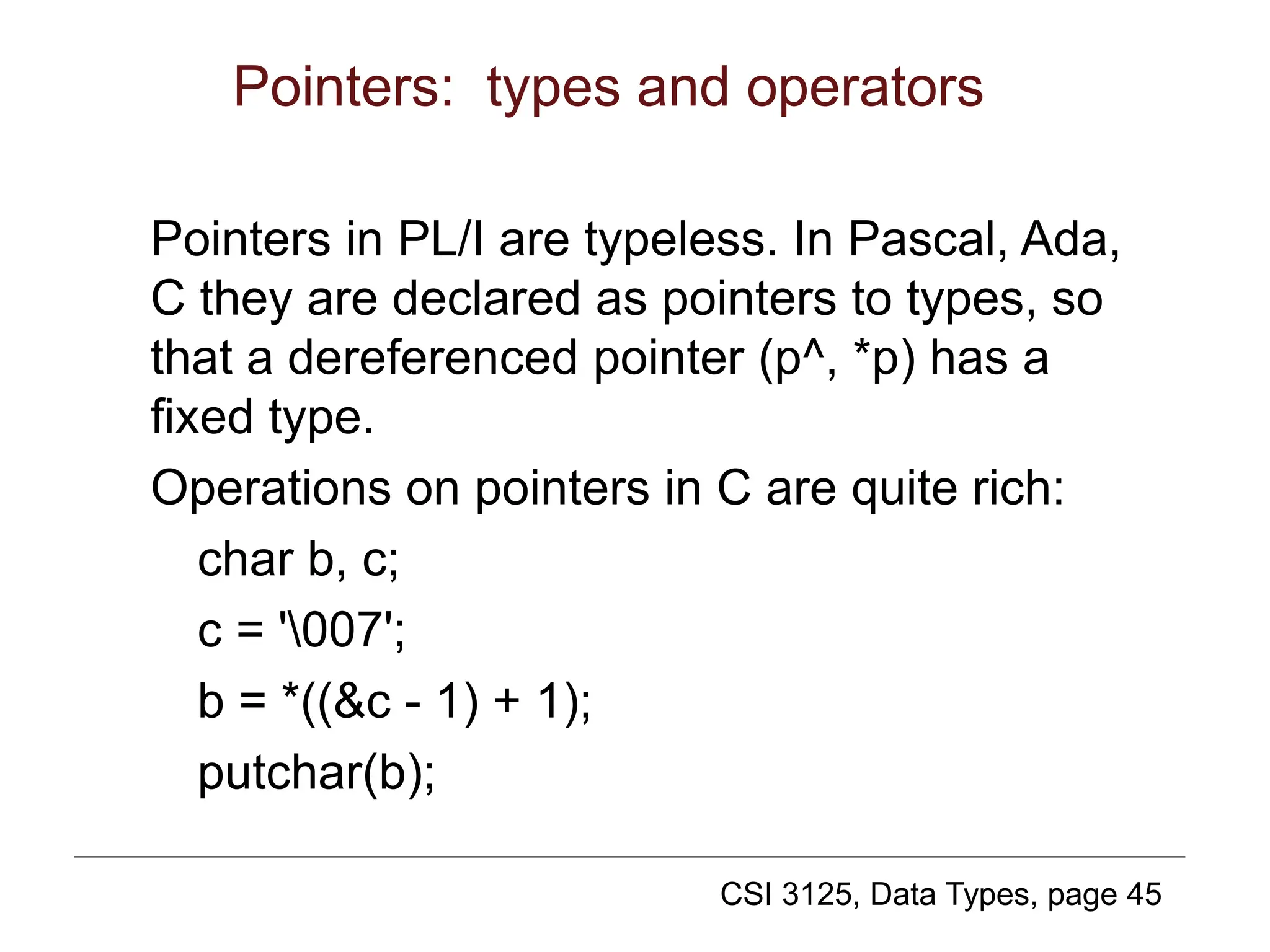
Back to pointers
[Note: We’re skipping 6.9.9]
A pointer variable has addresses as values (and a
special address nil or null for "no value"). They are used
primarily to build structures with unpredictable shapes
and sizes—lists, trees, graphs—from small fragments
allocated dynamically at run time.
A pointer to a procedure is possible, but normally we
have pointers to data (simple and composite). An
address, a value and usually a type of a data item
together make up a variable. We call it an anonymous
variable: no name is bound to it. Its value is accessed
by dereferencing the pointer.](https://image.slidesharecdn.com/09datatypes-240420100358-35269b6b/75/09_java_DataTypesand-associated-class-ppt-40-2048.jpg)