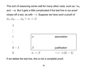
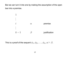
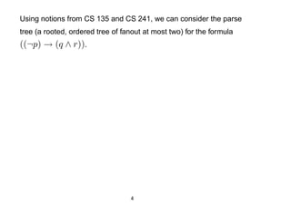
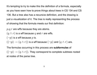
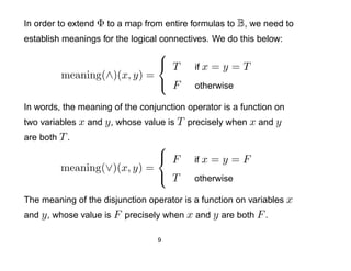
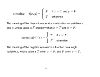
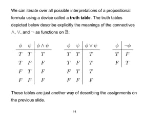
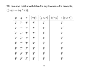
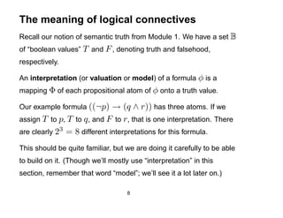
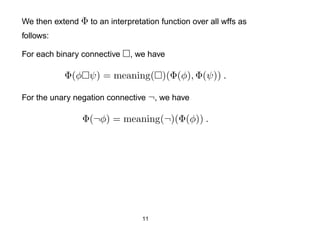
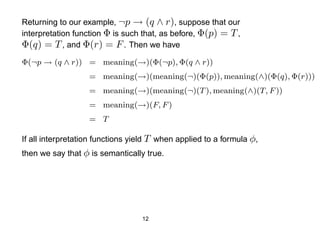
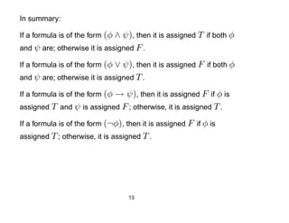
The document discusses the semantics of propositional logic, including: 1) Defining logical formulas using a formal language and grammar; 2) Describing the meaning of logical connectives like conjunction and negation through truth tables; 3) Explaining how interpretations assign truth values to formulas based on the truth values of their components.

1. The semantics of propositional logic
Readings: Sections 1.3 and 1.4 of Huth and Ryan.
In this module, we will nail down the formal definition of a logical
formula, and describe the semantics of propositional logic, which
will be familiar to you from Math 135 and CS 251. Our final goal is to
prove the soundness and completeness of propositional logic, but to
do that, we need to be precise about induction, which we review
carefully.
1

2. The formal language of formulas (1.3)
Our formulas can be viewed as strings over an alphabet composed
of our atoms (p, q, r, p1 , p2 , . . .), plus the symbols ¬, ∧, ∨, →,
and the open and close parentheses, ( and ). (⊥ is a convenience
in our proofs, and shouldn’t appear in formulas.)
In the previous module we gave a grammar for the well-formed
formulas of propositional logic:
φ ::= p | φ ∧ φ | φ ∨ φ | ¬φ | φ → φ
Recall that p ranges over all atoms and φ ranges over all
well-formed formulas (wffs) (that is, formulas that conform to the
grammar).
2

3. Also recall the notions of abstract syntax and operator precedence
that we discussed in Module 2, and our use of parentheses to
explicitly indicate precedence when necessary.
3

4. Using notions from CS 135 and CS 241, we can consider the parse
tree (a rooted, ordered tree of fanout at most two) for the formula
((¬p) → (q ∧ r)).
4

5. It’s tempting to try to make this the definition of a formula, especially
as you have seen how to prove things about trees in CS 134 and CS
136. But a tree also has a recursive definition, and the drawing is
just a visualization of it. The tree is really representing the process
of showing that the formula meets our first definition:
p,q ,r are wffs because they are atoms.
(q ∧ r) is a wff because q and r are wffs.
(¬p) is a wff because p is.
((¬p) → (q ∧ r)) is a wff because (¬p) and (q ∧ r) are.
The formulas occurring in this process are subformulas of
((¬p) → (q ∧ r)). They correspond to complete subtrees rooted
at nodes of the parse tree.
5

6. Apart from reordering some of the lines in the justification on the
previous slide, there is no other way to show that our formula meets
the definition. Another way of saying this is that the parse tree is
unique.
This is true for every formula that satisfies the definition. This will be
important for our semantics. The textbook calls this the inversion
principle, meaning it is possible to invert the process of building
formulas.
The textbook asks you to take this on faith, but for those of little faith,
we will prove it in a little while, since we’ll have the tools to do so.
6

7. The ideas of a formal definition of a logical formula and a separate
semantics for assigning a truth value to such a formula come from
the work of Gottlob Frege in 1879, though the notation he used was
quite different.
Many mathematicians and philosophers built on Frege’s ideas,
including Bertrand Russell, Alfred North Whitehead, Ludwig
Wittgenstein, and Emil Post. Throughout their work, the notation
changed and evolved.
What we have presented here is now standard terminology, though
you will still see variations on it in other books (for example, the use
of ⊃ in place of →).
7

8. The meaning of logical connectives
Recall our notion of semantic truth from Module 1. We have a set B
of “boolean values” T and F , denoting truth and falsehood,
respectively.
An interpretation (or valuation or model) of a formula φ is a
mapping Φ of each propositional atom of φ onto a truth value.
Our example formula ((¬p) → (q ∧ r)) has three atoms. If we
assign T to p, T to q , and F to r , that is one interpretation. There
are clearly 23 = 8 different interpretations for this formula.
This should be quite familiar, but we are doing it carefully to be able
to build on it. (Though we’ll mostly use “interpretation” in this
section, remember that word “model”; we’ll see it a lot later on.)
8

9. In order to extend Φ to a map from entire formulas to B, we need to
establish meanings for the logical connectives. We do this below:

 T if x =y=T
meaning(∧)(x, y) =
 F otherwise
In words, the meaning of the conjunction operator is a function on
two variables x and y , whose value is T precisely when x and y
are both T .

 F if x =y=F
meaning(∨)(x, y) =
 T otherwise
The meaning of the disjunction operator is a function on variables x
and y , whose value is F precisely when x and y are both F .
9

10. 
 F if x = T and y = F
meaning(→)(x, y) =
 T otherwise
The meaning of the disjunction operator is a function on variables x
and y , whose value is F precisely when x = T and y = F .

 T if x =F
meaning(¬)(x) =
 F otherwise
The meaning of the negation operator is a function on a single
variable x, whose value is T when x = F , and F when x = T .
10

11. We then extend Φ to an interpretation function over all wffs as
follows:
For each binary connective , we have
Φ(φ ψ) = meaning( )(Φ(φ), Φ(ψ)) .
For the unary negation connective ¬, we have
Φ(¬φ) = meaning(¬)(Φ(φ)) .
11

12. Returning to our example, ¬p → (q ∧ r), suppose that our
interpretation function Φ is such that, as before, Φ(p) = T ,
Φ(q) = T , and Φ(r) = F . Then we have
Φ(¬p → (q ∧ r)) = meaning(→)(Φ(¬p), Φ(q ∧ r))
= meaning(→)(meaning(¬)(Φ(p)), meaning(∧)(Φ(q), Φ(r)))
= meaning(→)(meaning(¬)(T ), meaning(∧)(T, F ))
= meaning(→)(F, F )
= T
If all interpretation functions yield T when applied to a formula φ,
then we say that φ is semantically true.
12

13. In summary:
If a formula is of the form (φ ∧ ψ), then it is assigned T if both φ
and ψ are; otherwise it is assigned F .
If a formula is of the form (φ ∨ ψ), then it is assigned F if both φ
and ψ are; otherwise it is assigned T .
→ ψ), then it is assigned F if φ is
If a formula is of the form (φ
assigned T and ψ is assigned F ; otherwise, it is assigned T .
If a formula is of the form (¬φ), then it is assigned F if φ is
assigned T ; otherwise, it is assigned T .
13

14. We can iterate over all possible interpretations of a propositional
formula using a device called a truth table. The truth tables
depicted below describe explicitly the meanings of the connectives
∧, ∨, and ¬ as functions on B:
φ ψ φ∧ψ φ ψ φ∨ψ φ ¬φ
T T T T T T T F
T F F T F T F T
F T F F T T
F F F F F F
These tables are just another way of describing the assignments on
the previous slide.
14

15. We can also build a truth table for any formula – for example,
((¬p) → (q ∧ r)).
p q r (¬p) (q ∧ r) ((¬p) → (q ∧ r))
T T T F T T
T T F F F T
T F T F F T
T F F F F T
F T T T T T
F T F T F F
F F T T F F
F F F T F F
15

16. We read a truth table as follows: each row represents a possible
interpretation function Φ. In the leftmost columns, we find the
atomic statements. If there are n atomic statements, then the truth
table will have 2n rows, as there would then be 2n possible truth
assignments to those atomic statements, and therefore 2n possible
interpretation functions Φ.
Moving to the right, we obtain the values in each column by applying
the meaning functions for the logical connectives to the truth values
in the previous columns.
The last column denotes the truth assignment given by the
interpretation function to the entire formula. If all values in the last
column are T , then all interpretation functions map the formula to
T , and we say that the formula is semantically true.
16

17. When we proved a sequent φ1 , φ2 , . . . φn ψ , the idea was that
eventually we should be able to show that if all of φ1 , φ2 , . . . φn
were true, then ψ would also be true. Now we have a way of
describing a circumstance (a valuation) under which we can
evaluate the truth value of formulas.
This suggests that what we want to show is that any valuation which
makes φ1 , φ2 , . . . φn true should make ψ true.
If this is in fact the case, we write φ1 , φ2 , . . . φn |= ψ . (The
symbol |= is read “models”).
As we said in Module 1, the central question to be answered is,
what is the relationship between the two relations |= and ?
17

18. We define φ1 , φ2 , . . . φn |= ψ to mean that any valuation that
makes φ1 , φ2 , . . . φn true also makes ψ true. |= is also called the
semantic entailment relation.
Our goal is to prove that this is equivalent to our previous notion of
valid sequents.
The property that if φ1 , φ2 , . . . φn ψ , then φ1 , φ2 , . . . φn |= ψ
is called soundness.
The property that if φ1 , φ2 , . . . φn |= ψ , then φ1 , φ2 , . . . φn ψ
is called completeness.
18

19. Soundness states that any valid sequent says something about the
relationship between the formulas involved, under all valuations.
Completeness states that given a relationship between the
valuations of formulas, there must exist a proof of validity of the
corresponding sequent.
It helps to think about the case where n (the number of formulas on
the left-hand side) is zero. Soundness states that any formula that is
a theorem is true under all valuations. Completeness says that any
formula that is true under all valuations is a theorem.
We are going to prove these two properties for our system of natural
deduction and our system of valuations.
19

20. The completeness and soundness of propositional logic (not the
particular proof system we are studying, but an equivalent one) was
shown by Emil Post in his PhD thesis in 1920. (Post went on to
make contributions to early theoretical computer science, some of
which you may encounter in CS 360 and CS 365.)
We will follow the proofs of completeness and soundness given in
the textbook. These use the mathematical tool of induction, which
was introduced in Math 135 and discussed in CS 134 and CS 136,
but which deserves careful review.
20

21. Induction
Induction is used to prove some property M that depends on some
integer n; that is, M (n) is a statement about n. For example,
M (n) might be “Every even number greater than 2 but less than n
is the sum of two primes”.
The principle of mathematical induction says that if M (1) is true
(this is the base case), and in addition we can show that for any
n ≥ 1, if M (n) is true, then M (n + 1) is true (this is the inductive
step), then we can conclude that M (n) is true for all natural
numbers n. (We don’t actually know how to do this for the specific
statement M (n) above, which is called “Goldbach’s conjecture”.)
Induction is a way of proving (in a mathematical sense) statements
about an infinite number of situations or an infinite set.
21

22. We cannot prove the principle of mathematical induction; it is part of
the definition of natural numbers. (We will make this idea more
concrete later on in the course.)
One proof by induction you may have seen previously is the proof
that the sum of the first n natural numbers is n(n + 1)/2. This is
reproduced in our textbook (Theorem 1.31).
You may have also seen that there were many different forms of
induction, all equivalent to the basic form. We can vary the base
case and we can vary the inductive step.
Since we will eventually be formalizing induction as a well-defined
axiom of the natural numbers, we must be careful that all other
notions of induction we consider follow from the basic definition, in
order that our inductive reasoning will be justified.
22

23. We could, for instance, declare the base case to be proving that
M (3) is true, and have the inductive step show that for n ≥ 3,
M (n) being true implies M (n + 1) being true. The result proves
that M (n) is true for all n ≥ 3.
Given such a proof, we can define the property P such that
P (n) = M (n + 2), and then mechanically translate the proof
involving M to a proof involving P . The base case of that proof
would be proving P (1) true, and the inductive step would show that
for n ≥ 3, if P (n − 2) is true, then P (n − 1) is true, claiming a
conclusion that P (n − 2) is true for all n ≥ 3.
23

24. Now the additional substitution m = n − 2 makes this into a proof
that shows that P (1) is true, and for m ≥ 1, P (m) being true
implies that P (m + 1) is true. The conclusion becomes that P (m)
is true for all m ≥ 1. This is the basic form of induction, and so this
proof is valid. By reversing all our steps, we can show that the
original proof is also valid.
A similar technique works to show that if we have a proof that keeps
the base case of showing M (1) true, but modifies the inductive
step to show that for n ≥ 2, M (n − 1) being true implies M (n)
true. Again, a suitable set of mechanical substitutions gets us to the
basic form. This form might be preferable for certain properties M
where the algebra or other reasoning is simplified going from
M (n − 1) to M (n).
24

25. There is a form called “simultaneous induction”, in which two (or
more) statements are proved for all n.
As an example, we may have properties M1 (n) and M2 (n). The
base case proves both M1 (1) and M2 (1). The inductive step
assumes both M1 (n) and M2 (n), and uses these assumptions to
prove both M1 (n + 1) and M2 (n + 1). The conclusion reached
is that M1 (n) is true for all n, and M2 (n) is also true for all n.
By defining P (n) to be the property “M1 (n) is true and M2 (n) is
true”, we can mechanically reduce the above proof to the basic form.
25

26. The inductive step in basic induction is of the form “Assume P (n)
true and use it to prove P (n + 1) true.” From this, we conclude that
P (n) is true for all n. Sometimes, the induction is phrased in the
following form.
“Assume P (n) is not true for all n. Let n0 be the smallest value of
n for which P (n) does not hold. Thus P (n0 ) does not hold, but
P (n0 − 1) does. If, from these two facts, we can derive a
contradiction, our assumption must be wrong, and P (n) must hold
for all n.”
This argument wraps basic induction in a proof by contradiction. It is
sometimes called “proof by minimal counterexample”. It shows up,
for instance, in CS 341, in the discussion of greedy algorithms.
26

27. Our basic form of induction is sometimes called “weak induction”, in
contrast with a form called “strong induction”. (The adjectives refer
to the strength of the hypothesis in the inductive step.)
In the version of strong induction done in Math 135, the base case
shows that M (1) is true, and the inductive step (for n ≥ 1)
assumes M (1), M (2), . . . M (n) are true, and uses that
assumption to conclude M (n + 1) is true. Strong induction then
allows the conclusion that M (n) is true for all n.
Given such a proof, we can convert it to the basic form by defining
the property P (n) to be “M (m) is true for all m ≤ n”. All of these
forms are equivalent; we just choose the one that is most suitable
for our purposes.
27

28. Finally, there is a variation called “structural induction”. You saw this
in CS 134 or CS 136, where it was used to prove things about
binary trees.
Recall that a binary tree is a collection of nodes that is either empty,
or partitioned into three sets: a root, a left subtree, and a right
subtree (the last two being binary trees).
You saw proofs of facts such as “in a non-empty binary tree, the
number of leaves is one more than the number of nodes with exactly
two children” with a base case of the empty tree, and an inductive
step of assuming this was true of the left and right subtrees of a
non-empty tree and proving it is true of the whole tree.
28

29. Structural induction, for a property of some structure defined by a
recursive definition, is just strong induction on the number of times
that the definition is invoked in order to justify a particular structure.
In the case of binary trees, a justification that a nonempty tree T
satisfies the definition includes justifications that its left and right
subtrees are also binary trees. Those justifications thus each use
the definition fewer times than the justification for T .
We can do something similar to prove properties of formulas,
because we have a recursive definition for them. When we use
structural induction to prove a property M of a formula of the form
φ ∧ ψ , we assume M is true of φ and ψ and use that to prove M
is true for φ ∧ ψ . This is strong induction on the number of times
the definition is used to show a formula is well-formed.
29

30. What we have called “strong induction”, the textbook calls
“course-of-values induction”, and it also justifies structural induction
by talking about the height of the parse tree, instead of the number
of applications of the definition (which would correspond to the
number of nodes in the tree).
However, these are minor details. The point is that we have
structural induction to use in order to prove properties of formulas.
Structural induction will prove useful in courses such as CS 341, CS
360, and CS 466. But all of these forms of induction are just
different ways of expressing basic (“weak”) induction. We choose
the form that is most clear.
30

31. Soundness
Recall our definition of soundness: if φ1 , φ2 , . . . φn ψ , then
φ1 , φ2 , . . . φn |= ψ .
Soundness asserts that a valid sequent says something about
valuations. A sequent is shown valid by means of a natural
deduction proof. Our proof of soundness will proceed by induction
on the length of this proof (the number of lines).
Note that our proofs are just flattened trees. We could have given a
recursive definition of what a proof was (an application of a rule to
one or more subproofs) in which case our proof by induction
becomes structural induction. It might help to keep this in mind.
31

32. Thm: If φ1 , φ2 , . . . φn ψ , then φ1 , φ2 , . . . φn |= ψ .
Pf: If a sequent has a proof, then it has a proof that uses only the
core deduction rules (i.e., no MT, LEM, PBC, or ¬¬i). We shall
therefore assume that that the given proof of φ uses only core
deduction rules and proceed by strong induction on the length k of a
proof of the sequent φ1 , φ2 , . . . φn ψ.
If the proof has one line, it must be of the form
1 φ premise
So the sequent is φ φ, and clearly φ |= φ.
32

33. For the inductive step, we assume that soundness holds for
sequents with proofs of length less than k , and prove that it holds
for a sequent φ1 , φ2 , . . . φn ψ with a proof of length k (again,
our attention is restricted to deductions involving only core rules).
The k th line of the proof must look like
k ψ justification
We have a number of cases depending on which rule is applied in
this line. We’ll do enough cases to get the general idea, since we
have a lot of rules in natural deduction. (This proof is easier for other
systems with fewer rules, but then using such systems is more
difficult.)
33

34. If the k th line looks like
k ψ ∧ i k1 , k2
then ψ must be of the form ψ1 ∧ ψ2 , where ψ1 appears on line k1 ,
and ψ2 appears on line k2 .
The sequent φ1 , φ2 , . . . , φn ψ1 has a proof of length at most k1
(the first k1 lines of the proof we started with), so
φ1 , φ2 , . . . , φn |= ψ1 . Similarly, φ1 , φ2 , . . . , φn |= ψ2 .
What this means is that for every interpretation Φ such that
Φ(φ1 ) = T, . . . , Φ(φn ) = T , we also have Φ(ψ1 ) = T , and
whenever Φ(φ1 ) = T, . . . , Φ(φn ) = T , we have Φ(ψ2 ) = T .
34

35. So let Φ(φ1 ) = · · · = Φ(φn ) = T .
Then Φ(ψ1 ) = Φ(ψ2 ) = T . Therefore,
Φ(ψ1 ∧ψ2 ) = meaning(∧)(Φ(ψ1 ), Φ(ψ2 )) = meaning(∧)(T, T ) = T .
Thus, φ1 , φ2 , . . . , φn |= ψ , as required.
35

36. This sort of reasoning works well for many other rules, such as ∧e1
and →e. But it gets a little complicated if the last line in our proof
closes off a box, as with →i. Suppose we have such a proof of
φ1 , φ2 , . . . , φn α → β.
1
.
.
.
i α assumption
.
.
.
k−1 β justification
k α→β → i i–(k − 1)
If we delete the last line, this is not a complete proof.
36

37. But we can turn it into one by making the assumption of the open
box into a premise.
1
.
.
.
i α premise
.
.
.
k−1 β justification
This is a proof of the sequent φ1 , φ2 , . . . , φn , α β.
37

38. Since our proof of φ1 , φ2 , . . . , φn , α β has k − 1 lines, we can
apply the inductive hypothesis to conclude that
φ1 , φ2 , . . . , φn , α |= β .
We need to conclude that φ1 , φ2 , . . . , φn |= α → β . So consider
an interpretation Φ that makes φ1 , φ2 , . . . , φn true. The only way
we could have Φ(α → β) = F would be if Φ(α) = T and
Φ(β) = F (this is by examination of the truth table that defines
meaning(→)). But we have
φ1 , φ2 , . . . , φn , α |= β ,
= · · · = Φ(φn ) = Φ(α) = T , then Φ(β) = T .
so if Φ(φ1 )
Hence Φ(α → β) = T , and we have φ1 , φ2 , . . . , φn |= α → β .
38

39. This sort of reasoning works for the cases where the last line closes
off a proof box.
The full proof involves a complete examination of each of the dozen
or so rules of natural deduction, but we have already seen the two
main ideas.
Soundness gives us a method of showing that a sequent
φ1 , φ2 , . . . , φn
ψ does not have a proof in natural deduction;
we simply have to find a valuation that makes φ1 , φ2 , . . . , φn true
but ψ false.
39

40. It is worth noting that the the proof of soundness given here for
classical deductions actually holds for both classical and intuitionist
proofs. An intuitionist proof is simply one that does not employ the
¬¬e rule; hence any intuitionist proof is also a classical proof, and
therefore soundness for intuitionism is an easy consequence of
soundness for classicism.
40

41. Completeness
Thm: If φ1 , φ2 , . . . φn |= ψ , then φ1 , φ2 , . . . φn ψ.
Proof: The proof is divided into three stages.
The first stage shows that if φ1 , φ2 , . . . φn |= ψ , then
|= φ1 → (φ2 → (. . . (φn → ψ) . . .)).
The second stage shows that if |= η , then η , for any formula η
(including those looking like what the first stage produced). If |= η ,
then η is called a tautology.
The third stage shows that if
φ1 → (φ2 → (. . . (φn → ψ) . . .)), then φ1 , φ2 , . . . φn ψ.
41

42. The first and third stages are the easiest, so let’s get them out of the
way. We first need to show that if φ1 , φ2 , . . . φn |= ψ , then
|= φ1 → (φ2 → (. . . (φn → ψ) . . .)).
How can we have Φ(φ1 → (φ2 → (. . . (φn → ψ) . . .))) = F
for an interpretation Φ? We would need Φ(φ1 ) = T and
Φ(φ2 → (φ3 → . . . (φn → ψ) . . .)) = F . We can continue to
unravel the formula, and conclude that
Φ(φ1 ) = Φ(φ2 ) = . . . = Φ(φn ) = T , and Φ(ψ) = F . But we
know φ1 , φ2 , . . . φn |= ψ , so this is impossible, by definition of |=.
For the third stage, we must take a proof of
φ1 → (φ2 → (. . . (φn → ψ) . . .)), and from it construct a
proof of φ1 , φ2 , . . . φn ψ .
42

43. This can be done simply by augmenting the proof of
φ1 → (φ2 → (. . . (φn → ψ) . . .)) with n lines at the
beginning introducing φ1 , φ2 , . . . φn as premises, and n lines at
the end, each applying →e to peel off φ1 , then φ2 , and so on up to
φn , which leaves ψ as the last line. The result is a proof of
φ1 , φ2 , . . . φn ψ .
Technically speaking, both of these stages should be proofs by
induction on n, but they are so “iterative” or algorithmic in nature that
the induction will only obscure what is going on. This is also true in
the second stage, but there we also must do a structural induction
on formulas, so we really need to keep things as clear as possible.
43

44. The second stage is more complicated than anything we have done
so far, though it is not technically difficult. Our goal is to prove that
for any formula η , if |= η , then η.
Suppose η has n distinct propositional atoms. (This n is different
from the one in the first and third stages.) We are going to have to
construct a proof knowing only that each of the 2n interpretations
assign T to η . We do this by constructing 2n subproofs, one for
each interpretation, and then putting them all together.
An interpretation Φ assigns T or F to each of the atoms, which we’ll
call p1 , p2 , . . . , pn . (You can think of it as a line in a truth table for
η .) Relative to Φ, we define pi to be the formula pi if Φ(pi ) = T ;
ˆ
otherwise pi is the formula ¬pi . Hence, for all pi , Φ(ˆi ) = T .
ˆ p
44

45. The induction on formulas is contained in the following lemma:
Lemma (1.38): Let φ be a formula with propositional atoms
p1 , p2 , . . . pn , and Φ an interpretation. If Φ(φ) = T , then
p1 , p2 , . . . pn φ; if Φ(φ) = F , then p1 , p2 , . . . pn ¬φ.
ˆ ˆ ˆ ˆ ˆ ˆ
Note: this lemma and its proof are a great example of a proof by
simultaneous induction. As we shall see, we are really only
interested in the statement that if Φ(φ) = T , then
p1 , . . . , pn
ˆ ˆ φ. But in order to have enough information to prove
the result inductively, we must prove both claims.
45

46. Proof of the Lemma: By structural induction on the formula φ.
If φ is an atom p, the statement of the lemma says that p p and
¬p ¬p, which have one-line proofs.
If φ is of the form ¬φ1 , then we may apply the inductive hypothesis
to φ1 . If Φ(φ) = T , then Φ(¬φ1 ) = T , which means that
Φ(φ1 ) = F .
By the inductive hypothesis, p1 , p2 , . . . pn
ˆ ˆ ˆ ¬φ1 .
But this just says p1 , p2 , . . . pn
ˆ ˆ ˆ φ, as required.
If Φ(φ) = F , then Φ(φ1 ) = T , and we get p1 , p2 , . . . pn φ1 .
ˆ ˆ ˆ
Adding an application of ¬¬i gives p1 , p2 , . . . pn ¬¬φ1 , which
ˆ ˆ ˆ
is p1 , p2 , . . . pn ¬φ.
ˆ ˆ ˆ
46

47. In the remaining cases, φ is of the form φ1 ◦ φ2 . These are all
similar; we will do only one here, where φ is of the form φ1 → φ2 .
(Unlike with the proof of soundness, the textbook treats all the
cases.)
Let q1 , . . . , qk be the propositional atoms of φ1 and r1 , . . . r be
the propositional atoms of φ2 . First, we treat the case where
Φ(φ) = F . Then Φ(φ1 ) = T and Φ(φ2 ) = F .
Applying the inductive hypothesis, we have q1 , . . . , qk
ˆ ˆ φ1 , and
r1 , . . . , r
ˆ ˆ ¬φ2 . Since both of the sets of mini-formulas on the
left-hand sides of the sequents are subsets of p1 . . . pn , we know
ˆ ˆ
that p1 , . . . , pn φ1 , and p1 , . . . , pn ¬φ2 . We can put these
ˆ ˆ ˆ ˆ
proofs together with one application of ∧i to show
p1 , . . . , pn φ1 ∧ ¬φ2 .
ˆ ˆ
47

48. We’ve shown p1 , . . . , pn
ˆ ˆ φ1 ∧ ¬φ2 . But what we need to show
is p1 , . . . , pn ¬(φ1 → φ2 ). All we need is a proof of
ˆ ˆ
φ1 ∧ ¬φ2 ¬(φ1 → φ2 ). The book leaves this as an exercise.
That was the subcase where Φ(φ) = Φ(φ1 → φ2 ) = F . If
Φ(φ) = T , there are three possibilities for Φ(φ1 ) and Φ(φ2 ): TT,
FT, and FF. Each of these, using the same sort of reasoning,
generates a sequent which is close to what we need; for example,
TT generates p1 , . . . , pn
ˆ ˆ φ1 ∧ φ2 , and thus generates the
exercise φ1 ∧ φ2 φ1 → φ2 .
We then have to consider the cases where φ is of the form φ1 ∧ φ2
or φ1 ∨ φ2 . In total, eleven exercises are generated for future
practice in natural deduction. That concludes the proof of the
lemma, which is not difficult, but rather tedious.
48

49. Given the lemma, we can prove the main part of stage 2, which is to
show that if |= η , then η . Since η is a tautology, all 2n possible
valuations make it true. Thus for every possible choice for
p1 , p2 , . . . , pn , we can use the lemma to get a proof of
ˆ ˆ ˆ
p 1 , p2 , . . . , pn η .
ˆ ˆ ˆ
To get a proof of η , we use LEM to obtain p1 ∨ ¬p1 . Then we
open two proof boxes with assumptions p1 and ¬p1 , with the
intention of using ∨e on them. (Though we have to do this
sequentially, think of them as happening in parallel.)
Within each of those, we use LEM to obtain p2 ∨ ¬p2 , and do the
same thing, nesting boxes. At the innermost level, we’ll have 2n
boxes side by side, each one with assumptions accumulating one
choice for each of p1 , p2 , . . . , pn .
ˆ ˆ ˆ
49

50. For each one of the 2n innermost boxes, there are n enclosing
proof boxes making assumptions that build up one choice of
p 1 , p2 , . . . , pn .
ˆ ˆ ˆ
Thus we can fill each one with one of the proofs provided by the
lemma to conclude η within the innermost boxes. We then close the
innermost proof boxes in pairs with ∨e, concluding η . Then we
close the next matching pairs with ∨e, concluding η , and so on at
each level, until all the proof boxes are closed.
The next slide illustrates this for the case n = 2.
50

51. 1 p1 ∨ ¬p1 LEM
2 p1 ass ¬p1 ass
3 p2 ∨ ¬p2 LEM p2 ∨ ¬p2 LEM
4 p2 ass ¬p2 ass p2 ass ¬p2 ass
.
. .
. .
. .
.
5 . . . .
6
7 η η η η
8 η ∨e η ∨e
9 η ∨e
51

52. The resulting proof is not one of which we should be particularly
proud. But it is a valid proof of η.
This concludes the second stage, and thus the entire proof of the
completeness of propositional logic. We have shown that if
φ1 , φ2 , . . . , φn |= ψ , then φ1 , φ2 , . . . , φn ψ.
Putting this together with soundness, we see that
φ1 , φ2 , . . . , φn |= ψ if and only if φ1 , φ2 , . . . , φn ψ . Our two
notions, proof by natural deduction (syntactic transformations) and
semantics via truth-table valuations, have been shown to coincide.
The next language for which we describe a proof system and
semantics, predicate logic, is also sound and complete, but the
proofs of those properties are beyond the scope of this course.
52

53. What about intuitionist reasoning?
Notice how, in the proof of the completeness of propositional proof
theory with respect to truth-table semantics, we made several
appeals to LEM—one for each atom, in fact. Thus, the proof of
completeness, as given, does not hold for intuitionist logic.
This should come as no suprise, since, upon a moment’s reflection,
we must realize that inuitionist logic is not complete with respect to
truth-table semantics.
For a counterexample to completeness for intuitionist logic, it simply
suffices to consider LEM. We know that LEM is not a theorem of
intuitionist proof theory (i.e., φ ∨ ¬φ under intuitionism), and yet
truth-table semantics tell us that |= φ ∨ ¬φ.
53

54. We could also consider as a counterexample the classical theorem
(φ → ψ) ∨ (ψ → φ), which we discussed previously. We have
already shown that this formula has a classical proof; hence, by
soundness, |= (φ → ψ) ∨ (ψ → φ). But the statement has no
intuitionist proof, so again, the formula demonstrates the
incompleteness of intuitionist reasoning with respect to truth-table
semantics.
It is clear, then, that any completeness proof for propositional logic
with respect to truth-table semantics must include an appeal to
LEM, or one of its equivalents (¬¬e or PBC); otherwise, it would
also be a proof of the completeness of intuitionist reasoning with
respect to truth-table semantics, which we know to be false.
54

55. Intuitionist semantics?
This discussion may lead us to wonder whether we can find some
other semantics for propositional logic that yields truth on exactly
the intuitionist theorems.
The answer is yes, but the associated semantics is much more
mathematically involved than simple truth table semantics. One way
to do it is via the use of structures called Heyting algebras (which
are a generalization of the Boolean algebra of T and F , upon which
classical reasoning is based).
One specific example of a semantics for intuitionist logic is a map
from each atom in a given formula into an open subset of the real
plane (R2 ), rather than simply T or F . The logical connectives then
have meanings phrased as operations on such sets.
55

56. Intuitionist semantics
Then a formula is an intuitionist theorem if and only if its image
under this map is always R2 , regardless of which open sets are
assigned to the individual atoms.
As a result, intuitionist reasoning is both sound and complete with
respect to Heyting algebra semantics.
Turning our attention once more to classical reasoning, since there
are classical theorems that are not intuitionist theorems (but not vice
versa), we discover that classical reasoning is complete, but not
sound with respect to Heyting algebra semantics.
56

57. We can summarize the relationships between the proof systems
and semantic models as follows:
Truth-Table Semantics Heyting Algebra Semantics
Classical Logic Sound and Complete Complete, but not Sound
Intuitionist Logic Sound, but not Complete Sound and Complete
57

58. What’s coming next?
Before we move to predicate logic, we will briefly discuss the parts
of Chapter 1 that we are not covering in depth. We will also survey
some alternate proof systems, and some implications of the material
we have just covered, particularly as it relates to topics in other CS
courses.
The definitions of both the system of natural deduction for predicate
logic and the semantics associated with these more expressive
formulas will prove to be considerably more complicated.
58

59. Goals of this module
You should understand the semantics presented for propositional
logic in terms of interpretations, and you should be very clear on the
distinction between a formula being semantically true and a formula
being syntactically provable.
You should be comfortable with the various forms of induction
discussed, particularly structural induction, and be able to do such
proofs yourself.
You should be able to fill in any of the holes left in the proofs of
soundness and completeness, both in terms of understanding the
big picture (what needs to go into the holes in order to complete the
proof structure), and the specific details.
59