1. Distribution and Population Dynamics of
Tribolium castaneum
Sharon M. Perera
Department of Environmental Science and Policy
Faculty Sponsor: Alan Hastings Ph.D.
INTRODUCTION RESULTS DISCUSSION
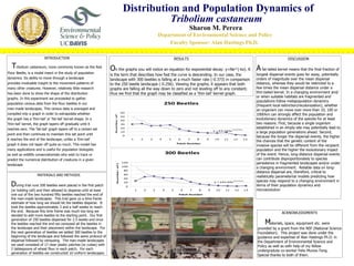
Tribolium castaneum, more commonly known as the Red On the graphs you will notice an equation for exponential decay: y=Ne^(-kx). K A fat-tailed kernel means that the final fraction of
Flour Beetle, is a model insect in the study of population longest dispersal events goes far away, potentially
is the term that describes how fast the curve is descending. In our case, the
dynamics. Its ability to move through a landscape landscape with 300 beetles is falling at a much faster rate (-0.373) in comparison orders of magnitude over the mean dispersal
provides invaluable insight to the movement patterns of to the 250 beetle landscape (-0.256). Viewing the graphs, it appears that both distance, whereas they would be restricted to a
many other creatures. However, relatively little research graphs are falling all the way down to zero and not leveling off to any constant; few times the mean dispersal distance under a
has been done to show the shape of the distribution thus we find that the graph may be classified as a ‘thin-tail’ kernel graph. thin-tailed kernel. In a changing environment and/
graphs. In this experiment we proceeded to gather
or when suitable habitats are fragmented and
populations follow metapopulation dynamics
250 Beetles
Number of Beetles
population census data from the flour beetles in our
(frequent local extinction/recolonization), whether
man-made landscapes. This census data is averaged and an organism can move over more than 10, 100 or
60
compiled into a graph in order to extrapolate whether
1000km can strongly affect the population and
50
the graph has a ‘thin-tail’ or ‘fat-tail’ kernel shape. In a 40 evolutionary dynamics of the species for at least
‘thin-tail’ kernel, the graph tapers off gradually until it 30 two reasons. First, because a single organism
reaches zero. The ‘fat-tail’ graph tapers off to a certain set 20
-0.2556x
established in an empty site may potentially lead to
y = 63.144e
10 a large population generations ahead. Second,
point and then continues to maintain this set point until 0
because the longer the dispersal events, the higher
it reaches the end of the landscape; unlike a ‘thin-tail’ 1 2 3 4 5 6 7 8 9 10 11 12 13
the chances that the genetic content of the
Patch Number
graph it does not taper off quite so much. This model has invasive species will be different from the recipient
many applications and is useful for population biologists population and the higher the evolutionary impact
300 Beetles of the event. Hence, long-distance dispersal events
Number of Beetles
as well as wildlife conservationists who wish to track or
predict the numerical distribution of creatures in a given can contribute disproportionately to species
landscape
120 persistence in fragmented landscapes and/or under
100
a changing environment. Reliable data on long-
80
distance dispersal are, therefore, critical to
MATERIALS AND METHODS 60
realistically parameterize models predicting how
40
species may respond to a changing environment in
During trial runs 200 beetles were placed in the first patch
-0.3731x
20 y = 143.44e
0 terms of their population dynamics and
(or holding cell) and then allowed to disperse until at least 1 2 3 4 5 6 7 8 9 10 11 12 13 microevolution
one out of the two hundred fifty beetles reached the end of Patch Number
the man-made landscapes. This trial gave us a time frame
estimate of how long we should let the beetles disperse. It
took the beetles approximately 3 and a half weeks to reach
the end. Because this time frame was much too long we ACKNOWLEDGMENTS
decided to add more beetles to the starting point. Our first
Materials, space, equipment etc. were
generation of 250 beetles dispersed for 2.5 weeks and once
the beetles reached the end we censused all the beetles in
the landscape and their placement within the landscape. For provided by a grant from the NSF (National Science
the next generation of beetles we added 300 beetles to the Foundation). This project was done under the
beginning of the landscape and followed the same protocol of guidance and expertise of Alan Hastings Ph.D. in
dispersal followed by censusing. The man-made landscapes the Department of Environmental Science and
we used consisted of 17 clear plastic patches (or cubes) with Policy as well as with help of my fellow
2 tablespoons of wheat flour in each patch. For each
undergradute co-worker Felix Munox-Teng.
generation of beetles we constructed 10 uniform landscapes.
Special thanks to both of them.