SlideShare a Scribd company logo
1 of 37
Download to read offline
82
VI Benchmarking
A. Introduction
6.1. Benchmarking deals with the problem of com-
bining a series of high-frequency data (e.g., quarterly
data) with a series of less frequent data (e.g., annual
data) for a certain variable into a consistent time series.
The problem arises when the two series show incon-
sistent movements and the less frequent data are con-
sidered the more reliable of the two. The purpose of
benchmarking is to combine the relative strengths of
the low- and high-frequency data. While benchmark-
ing issues also arise in annual data (e.g., when a survey
is only conducted every few years), this chapter deals
with benchmarking to derive quarterly national
accounts (QNA) estimates that are consistent with
annual national accounts (ANA) estimates, where the
annual data1 provide the benchmarks.2 Quarterly data
sources often differ from those used in the correspond-
ing annual estimates, and the typical result is that
annual and quarterly data sources show inconsistent
annual movements. In a few cases, the quarterly data
may be superior and so may be used to replace the
annual data.3 More typically, the annual data provide
the most reliable information on the overall level and
long-term movements in the series, while the quarterly
source data provide the only available explicit4 infor-
mation about the short-term movements in the series,
so that there is a need to combine the information con-
tent of both the annual and quarterly sources.
6.2. Benchmarking has two main aspects, which in
the QNA context are commonly looked upon as two
different topics; these are (a) quarterization5 of
annual data to construct time series of historical QNA
estimates (“back series”) and revise preliminary
QNA estimates to align them to new annual data
when they become available, and (b) extrapolation to
update the series from movements in the indicator for
the most current period (“forward series”). In this
chapter, these two aspects of benchmarking are inte-
grated into one common benchmark-to-indicator
(BI) ratio framework for converting individual
indicator series into estimates of individual QNA
variables.
6.3. To understand the relationship between the cor-
responding annual and quarterly data, it is useful to
observe the ratio of the annual benchmark to the sum
of the four quarters of the indicator (the annual BI
ratio). Movements in the observed annual BI ratio
show inconsistencies between the long-term move-
ments in the indicator and in the annual data.6 As a
result, movements in the annual BI ratio can help
identify the need for improvements in the annual and
quarterly data sources. The technical discussion in
this chapter treats the annual benchmarks as binding
and, correspondingly, the inconsistencies as caused
by errors7 in the indicator and not by errors in the
annual data. Benchmarking techniques that treat the
benchmarks as nonbinding are briefly described in
Annex 6.1.
1That is, the annual source data, or ANA estimates based on a separate
ANA compilation system.
2A trivial case of benchmarking occurs in the rare case in which
annual data are available for only one year. In this case, consistency
can be achieved simply by multiplying the indicator series by a single
adjustment factor.
3One instance is annual deflators that are best built up from quarterly
data as the ratio between the annual sums of the quarterly current and
constant price data, as discussed in Chapter IX Section B. Another
case is that of nonstandard accounting years having a significant effect
on the annual data.
4The annual data contain implicit information on aspects of the short-
term movements in the series.
5Quarterization refers to generation of quarterly data for the back
series from annual data and quarterly indicators, and encompasses
two special cases, namely:
(a) Interpolation—that is, drawing a line between two points—which
in the QNA mainly applies to stock data (except in the rare case of
periodic quarterly benchmarks).
(b) Temporal distribution, that is, distributing annual flow data over
quarters.
6See Section B.4 of Chapter II for a further discussion of this issue.
7The errors can be systematic (“bias”) or irregular (“noise”).
6.4. The general objective of benchmarking is
• to preserve as much as possible the short-term
movements in the source data under the restrictions
provided by the annual data and, at the same time,
• to ensure, for forward series, that the sum of the
four quarters of the current year is as close as pos-
sible to the unknown future annual data.
It is important to preserve as much as possible the
short-term movements in the source data because the
short-term movements in the series are the central
interest of QNA, about which the indicator provides
the only available explicit information.
6.5. In two exceptional cases, the objective should
not be to maximally preserve the short-term move-
ments in the source data: (a) if the BI ratio is known
to follow a short-term pattern, for example, is subject
to seasonal variations; and (b) if a priori knowledge
about the underlying error mechanism indicates that
the source data for some quarters are weaker than
others and thus should be adjusted more than others.
6.6. As a warning of potential pitfalls, this chapter
starts off in Section B by explaining the unacceptable
discontinuities between years—the “step problem”—
caused by distributing annual totals in proportion to the
quarterly distribution (pro rata distribution) of the indi-
cator. The same problem arises if preliminary quarterly
estimates are aligned to the annual accounts by distrib-
uting the differences between the annual sums of the
quarterly estimates and independent annual estimates
for the same variable evenly, or pro rata, among the four
quarters of each year. Techniques that introduce breaks
in the time series seriously hamper the usefulness of
QNA by distorting the view of developments and pos-
sible turning points. They also thwart forecasting and
constitute a serious impediment for seasonal adjust-
ment and trend analysis. In addition to explaining the
step problem, section B introduces the BI ratio frame-
work that integrates quarterization and extrapolation
into one framework.
6.7. Subsequently, the chapter presents a BI ratio-
based benchmarking technique that avoids the step
problem (the “proportional Denton” technique with
extensions).8 The proportional Denton technique
generates a series of quarterly estimates as propor-
tional to the indicator. as possible subject to the
restrictions provided by the annual data. The chapter
goes on to propose an enhancement to the Denton
technique to better deal with the most recent periods.
Other enhancements to the Denton are also men-
tioned and some other practical issues are considered.
6.8. Given the general objective stated above it fol-
lows that, for the back series, the proportional Denton
is by logical consequence9 optimal, if
• maximal preservation of the short-term move-
ments in the indicator is specified as keeping the
quarterly estimates as proportional to the indicator
as possible; and
• the benchmarks are binding.
Under the same conditions, it also follows that for the
forward series, the enhanced version provides the best
way of adjusting for systematic bias and still maxi-
mally preserving the short-term movements in the
source data. In addition, compared with the alterna-
tives discussed in Annex 6.1, the enhanced propor-
tional Denton technique is relatively simple, robust,
and well suited for large-scale applications.
6.9. The technical discussion in this chapter also
applies to estimates based on periodically “fixed”
ratios in the absence of direct indicators for some
variables that also result in a step problem. As men-
tioned in Chapter III, these cases include cases in
which (a) estimates for output are derived from data
for intermediate consumption, or, estimates for inter-
mediate consumption are derived from data for out-
put; (b) estimates for output are derived from other
related indicators such as inputs of labor or particular
raw materials; and (c) ratios are used to gross up for
units not covered by a sample survey (e.g., establish-
ments below a certain threshold). In all these cases,
the compilation procedure can be expressed in a
benchmark-to-(related) indicator form, and annual,
or less frequent, variations in the ratios result in step
problems. The proportional Denton technique can
also be used to avoid this step problem and, for the
reasons stated above, would generally provide opti-
mal results, except in the case of potential seasonal
and cyclical variations in the ratios. This issue is dis-
cussed in more detail in Section D.1, which also pro-
vides a further enhancement to the proportional
Denton that allows for incorporation of a priori
known seasonal variations in the BI ratio.10
Introduction
83
9Because the proportional Denton is a mathematical formulation of
the stated objective.
10Further enhancements, which allow for incorporating a priori knowl-
edge that the source data for some quarters are weaker than others, and
thus should be adjusted more than others, are also feasible.
8Some of the alternative techniques that have been proposed are dis-
cussed in Annex 6.1, which explains the advantages of the propor-
tional Denton technique over these alternatives.
6.10. In the BI ratio benchmarking framework, only
the short-term movements—not the format and overall
level11—of the indicator are important, as long as they
constitute continuous time series.12 The quarterly indi-
cator may be in the form of index numbers (value, vol-
ume, or price) with a reference period that may differ
from the base period13 in the QNA; be expressed in
physical units; be expressed in monetary terms; or be
derived as the product of a price index and a volume
indicator expressed in physical units. In the BI frame-
work, the indicator only serves to determine the short-
term movements in the estimates, while the annual
data determine the overall level and long-term move-
ments. As will be shown, the level and movements in
the final QNA estimates will depend on the following:
• The movements, but not the level, in the short-term
indicator.
• The level of the annual data—the annual BI ratio—
for the current year.
• The level of the annual data—the annual BI
ratios—for several preceding and following years.
Thus, it is not of any concern that the BI ratio is not
equal to one,14 and the examples in this chapter are
designed to highlight this basic point.
6.11. While the Denton technique and its enhance-
ments are technically complicated, it is important to
emphasize that shortcuts generally will not be satis-
factory unless the indicator shows almost the same
trend as the benchmark. The weaker the indicator is,
the more important it is to use proper benchmarking
techniques. While there are some difficult concep-
tual issues that need to be understood before setting
up a new system, the practical operation of bench-
marking is typically automated15 and is not prob-
lematic or time-consuming. Benchmarking should
be an integral part of the compilation process and
conducted at the most detailed compilation level. It
represents the QNA compilation technique for
converting individual indicators into estimates of
individual QNA variables.
B. A Basic Technique for Distribution
and Extrapolation with an Indicator
6.12. The aim of this section is to illustrate the step
problem created by pro rata distribution and relate
pro rata distribution to the basic extrapolation with
an indicator technique. Viewing the ratio of the
derived benchmarked QNA estimates to the indica-
tor (the quarterly BI ratio) implied by the pro rata
distribution method shows that this method intro-
duces unacceptable discontinuities into the time
series. Also, viewing the quarterly BI ratios implied
by the pro rata distribution method together with the
quarterly BI ratios implied by the basic extrapola-
tion with an indicator technique shows how distrib-
ution and extrapolation with indicators can be put
into the same BI framework. Because of the step
problem, the pro rata distribution technique is not
acceptable.
1. Pro Rata Distribution and the Step Problem
6.13. In the context of this chapter, distribution
refers to the allocation of an annual total of a flow
series to its four quarters.A pro rata distribution splits
the annual total according to the proportions indi-
cated by the four quarterly observations. A numerical
example is shown in Example 6.1 and Chart 6.1.
6.14. In mathematical terms, pro rata distribution
can be formalized as follows:
Distribution presentation
(6.1.a)
or
Benchmark-to-indicator
ratio presentation (6.1.b)
where
Xq,β is the level of the QNA estimate for quarter q of
year β;
Iq,β is the level of the indicator in quarter q of year
β; and
Aβ is the level of the annual data for year β.
6.15. The two equations are algebraically equivalent,
but the presentation differs in that equation (6.1.a)
emphasizes the distribution of the annual benchmark
(Aβ) in proportion to each quarter’s proportion of the
q q
q
q
X I
A
I
, ,
,
β β
β
β
= ⋅






∑
q
q
q
q
X A
I
I
,
,
,
β β
β
β
= ⋅






∑
VI BENCHMARKING
84
11The overall level of the indicators is crucial for some of the alterna-
tive methods discussed in Annex 6.1.
12See definition in paragraph 1.13.
13For traditional fixed-base constant price data, see Chapter IX.
14In the simple case of a constant annual BI ratio, any level difference
between the annual sum of the indicator and the annual data can be
removed by simply multiplying the indicator series by the BI ratio.
15Software for benchmarking using the Denton technique is used in
several countries. Countries introducing QNA or improving their
benchmarking techniques, may find it worthwhile to obtain existing
software for direct use or adaptation to their own processing systems.
For example, at the time of writing, Eurostat and Statistics Canada
have software that implement the basic version of the Denton tech-
nique; however, availability may change.
annual total of the indicator16 (Iq,β /Σq
I4,β), while
equation (6.1.b) emphasizes the raising of each quar-
terly value of the indicator (Iq,β ) by the annual BI
ratio (Aβ /Σq
Iq,β).
6.16. The step problem arises because of disconti-
nuities between years. If an indicator is not growing
as fast as the annual data that constitute the bench-
mark, as in Example 6.1, then the growth rate in the
QNA estimates needs to be higher than in the indica-
tor. With pro rata distribution, the entire increase in
the quarterly growth rates is put into a single quarter,
while other quarterly growth rates are left unchanged.
The significance of the step problem depends on the
size of variations in the annual BI ratio.
2. Basic Extrapolation with an Indicator
6.17. Extrapolation with an indicator refers to using the
movementsintheindicatortoupdatetheQNAtimeseries
with estimates for quarters for which no annual data are
yet available (the forward series).A numerical example is
shown in Example 6.1 and Chart 6.1 (for 1999).
6.18. In mathematical terms, extrapolation with an
indicator can be formalized as follows, when moving
from the last quarter of the last benchmark year:
Moving presentation
(6.2.a)
or
BI ratio presentation
(6.2.b)
6.19. Again, note that equations (6.2.a) and (6.2.b)
are algebraically equivalent, but the presentation
differs in that equation (6.2.a) emphasizes that the
last quarter of the last benchmark year (X4,β ) is
extrapolated by the movements in the indicator from
that period to the current quarters (Iq,β +1/I4, β ), while
equation (6.2.b) shows that this is the same as
4 1 4 1
4
4
, ,
,
,
β β
β
β
+ +
= ⋅






X I
X
I
4 1 4
4 1
4
, ,
,
,
β β
β
β
+
+
= ⋅






X X
I
I
A Basic Technique for Distribution and Extrapolation with an Indicator
85
Example 6.1. Pro Rata Distribution and Basic Extrapolation
Indicator Derived QNA Estimates
Period-to- Period-to-
The Period Annual Annual Period
Indicator Rate of Data BI ratio Distributed Data Rate of
(1) Change (2) (3) (1) • (3) = (4) Change
q1 1998 98.2 98.2 • 9.950 = 977.1
q2 1998 100.8 2.6% 100.8 • 9.950 = 1,003.0 2.6%
q3 1998 102.2 1.4% 102.2 • 9.950 = 1,016.9 1.4%
q4 1998 100.8 –1.4% 100.8 • 9.950 = 1,003.0 –1.4%
Sum 402.0 4000.0 9.950 4,000.0
q1 1999 99.0 –1.8% 99.0 • 10.280 = 1,017.7 1.5%
q2 1999 101.6 2.6% 101.6 • 10.280 = 1,044.5 2.6%
q3 1999 102.7 1.1% 102.7 • 10.280 = 1,055.8 1.1%
q4 1999 101.5 –1.2% 101.5 • 10.280 = 1,043.4 –1.2%
Sum 404.8 0.7% 4161.4 10.280 4,161.4 4.0%
q1 2000 100.5 –1.0% 100.5 • 10.280 = 1,033.2 –1.0%
q2 2000 103.0 2.5% 103.0 • 10.280 = 1,058.9 2.5%
q3 2000 103.5 0.5% 103.5 • 10.280 = 1,064.0 0.5%
q4 2000 101.5 –1.9% 101.5 • 10.280 = 1,043.4 –1.9%
Sum 408.5 0.9% ? ? 4,199.4 0.9%
Pro Rata Distribution
The annual BI ratio for 1998 of 9.950 is calculated by dividing the annual output value (4000) by the annual sum of the indicator (402.0).This ratio is then used
to derive the QNA estimates for the individual quarters of 1998. For example, the QNA estimate for q1 1998 is 977.1, that is, 98.2 times 9.950.
The Step Problem
Observe that quarterly movements are unchanged for all quarters except for q1 1999, where a decline of 1.8% has been replaced by an increase of 1.5%. (In
this series, the first quarter is always relatively low because of seasonal factors.) This discontinuity is caused by suddenly changing from one BI ratio to anoth-
er, that is, creating a step problem.The break is highlighted in the charts, with the indicator and adjusted series going in different directions.
Extrapolation
The 2000 indicator data are linked to the benchmarked data for 1999 by carrying forward the BI ratio for the last quarter of 1999. In this case, where the BI
ratio was kept constant through 1999, this is the same as carrying forward the annual BI ratio of 10.280. For instance, the preliminary QNA estimate for the
second quarter of 2000 (1058.9) is derived as 103.0 times 10.280. Observe that quarterly movements are unchanged for all quarters.
(These results are illustrated in Chart 6.1.)
16The formula, as well as all subsequent formulas, applies also to flow
series where the indicator is expressed as index numbers.
VI BENCHMARKING
86
Chart 6.1. Pro Rata Distribution and the Step Problem
The Indicator and the Derived Benchmarked QNA Estimates
In this example, the step problem shows up as an increase in the derived series from q4 1998 to q1 1999 that is not matched by the move-
ments in the source data.The quarterized data erroneously show a quarter-to-quarter rate of change for the first quarter of 1999 of 1.5%
while the corresponding rate of change in source data is –1.8% (in this series, the first quarter is always relatively low because of seasonal
factors).
Benchmark-to-Indicator Ratio
It is easier to recognize the step problem from charts of the BI ratio,where it shows up as abrupt upward or downward steps in the BI ratios
between q4 of one year and q1 of the next year. In this example, the step problem shows up as a large upward jump in the BI ratio from q4
1998 to q1 1999.
1998 1999 2000
Indicator (left-hand scale)
QNA estimates derived
using pro rata distribution
(right-hand scale)
Back Series Forward Series
(The corresponding data are given in Example 6.1)
96
98
100
102
104
106
108
960
980
1,000
1,020
1,040
1,060
1,080
9.8
9.9
10.0
10.1
10.2
10.3
10.4
10.5
1998 1999 2000
scaling up or down the indicator (Iq,β +1) by the BI
ratio for the last quarter of the last benchmark year
(X4,β /I4,β ).
6.20. Also, note that if the quarterly estimates for the
last benchmark year X4,β were derived using the pro
rata technique in equation (6.1), for all quarters, the
implied quarterly BI ratios are identical and equal to
the annual BI ratio. That is, it follows from equation
(6.1) that
(X4,β/I4,β) = (Xq,β/Iq,β) = (Aβ/Σq
Iq,β).17
6.21. Thus, as shown in equations (6.1) and (6.2),
distribution refers to constructing the back series
by using the BI ratio for the current year as adjust-
ment factors to scale up or down the QNA source
data, while extrapolation refers to constructing the
forward series by carrying that BI ratio forward.
C. The Proportional Denton Method
1. Introduction
6.22. The basic distribution technique shown in
the previous section introduced a step in the series,
and thus distorted quarterly patterns, by making all
adjustments to quarterly growth rates to the first
quarter. This step was caused by suddenly chang-
ing from one BI ratio to another. To avoid this dis-
tortion, the (implicit) quarterly BI ratios should
change smoothly from one quarter to the next,
while averaging to the annual BI ratios.18
Consequently, all quarterly growth rates will be
adjusted by gradually changing, but relatively
similar, amounts.
2. The Basic Version of the Proportional Denton
Method
6.23. The basic version of the proportional Denton
benchmarking technique keeps the benchmarked
series as proportional to the indicator as possible by
minimizing (in a least-squares sense) the difference
in relative adjustment to neighboring quarters sub-
ject to the constraints provided by the annual
benchmarks. A numerical illustration of its opera-
tion is shown in Example 6.2 and Chart 6.2.
6.24. Mathematically, the basic version of the pro-
portional Denton technique can be expressed as19
(6.3)
under the restriction that, for flow series,20
.
That is, the sum21of the quarters should be equal to
the annual data for each benchmark year,22
where
t is time (e.g., t = 4y – 3 is the first quarter of year y,
and t = 4y is the fourth quarter of year y);
Xt is the derived QNA estimate for quarter t;
It is the level of the indicator for quarter t;
Ay is the annual data for year y;
β is the last year for which an annual benchmark is
available; and
T is the last quarter for which quarterly source data
are available.
X A y
t
t
T
y
=
∑ = ∈{ }
2
1
, .....β
min –
,... ,...
..., ,......
–
–
1 4
1
1
2
2
1 4
X X X
t
t
t
t
t
T
T
X
I
X
I
t T
β
β
( ) =






∈ ( )
{ }
∑
The Proportional Denton Method
87
17Thus, in this case, it does not matter which period is being moved.
Moving from (a) the fourth quarter of the last benchmark year, (b)
the average of the last benchmark year, or (c) the same quarter of
the last benchmark year in proportion to the movements in the indi-
cator from the corresponding periods gives the same results.
Formally, it follows from equation (6.1) that
18In the standard case of binding annual benchmarks.
q
q
q
q
q
q
q
q
X X
I
I
X
I
I
A
I
I
, ,
,
,
,
,
,
,
,
β β
β
β
β
β
β
β
β
β
+
+
+
+
= ⋅






= ⋅






= ⋅








∑
1 4
1
4
1
1
19This presentation deviates from Denton’s original proposal by omit-
ting the requirement that the value for the first period be predeter-
mined.As pointed out by Cholette (1984), requiring that the values for
the first period be predetermined implies minimizing the first correc-
tion and can in some circumstances cause distortions to the bench-
marked series. Also, Denton’s original proposal dealt only with
estimating the back series.
20For the less common case of stock series, the equivalent constraint is
that the value of the stock at the end of the final quarter of the year is
equal to the stock at the end of the year. For index number series, the con-
straint can be formulated as requiring the annual average of the quarters
to be equal to the annual index or the sum of the quarters to be equal to
four times the annual index. The two expressions are equivalent.
21Applies also to flow series in which the indicator is expressed as
index numbers; the annual total of the indicator should still be
expressed as the sum of the quarterly data.
22Theannualbenchmarksmaybeomittedforsomeyearstoallowforcases
in which independent annual source data are not available for all years.
6.25. The proportional Denton technique implicitly
constructs from the annual observed BI ratios a time
series of quarterly benchmarked QNA estimates-to-
indicator (quarterly BI) ratios that is as smooth as
possible and, in the case of flow series:
• For the back series, (y  {1,...β}) averages23 to the
annual BI ratios for each year y.
• For the forward series, (y  {β + 1.....}) are kept
constant and equal to the ratio for the last quarter of
the last benchmark year.
We will use this interpretation of the proportional
Denton method to develop an enhanced version in the
next section.
6.26. The proportional Denton technique, as pre-
sented in equation (6.3), requires that the indicator
contain positive values only. For series that contain
zeroes but not negative values, this problem can be
circumvented by simply replacing the zeroes with
values infinitesimally close to zero. For series that
can take both negative and positive values, and are
derived as differences between two non-negative
series, such as changes in inventories, the problem
can be avoided by applying the proportional Denton
method to the opening and closing inventory levels
rather than to the change. Alternatively, the problem
can be circumvented by temporarily turning the indi-
cator into a series containing only positive values by
adding a sufficiently large constant to all periods,
benchmarking the resulting indicator using equation
(6.3), and subsequently deducting the constant from
the resulting estimates.
6.27. For the back series, the proportional Denton
method results in QNA quarter-to-quarter growth
rates that differ from those in the indicator (e.g., see
VI BENCHMARKING
88
Example 6.2. The Proportional Denton Method
Same data as in Example 6.1.
Indicator Estimated
The Period-to-Period Annual Annual BI Derived QNA Quarterly Period-to-Period
Indicator Rate of Change Data Ratios Estimates BI ratios Rate of Change
q1 1998 98.2 969.8 9.876
q2 1998 100.8 2.6% 998.4 9.905 3.0%
q3 1998 102.2 1.4% 1,018.3 9.964 2.0%
q4 1998 100.8 –1.4% 1,013.4 10.054 –0.5%
Sum 402.0 4000.0 9.950 4,000.0
q1 1999 99.0 –1.8% 1,007.2 10.174 –0.6%
q2 1999 101.6 2.6% 1,042.9 10.264 3.5%
q3 1999 102.7 1.1% 1,060.3 10.325 1.7%
q4 1999 101.5 –1.2% 1,051.0 10.355 –0.9%
Sum 404.8 0.7% 4161.4 10.280 4,161.4 4.0%
q1 2000 100.5 –1.0% 1,040.6 10.355 –1.0%
q2 2000 103.0 2.5% 1,066.5 10.355 2.5%
q3 2000 103.5 0.5% 1,071.7 10.355 0.5%
q4 2000 101.5 –1.9% 1,051.0 10.355 –1.9%
Sum 408.5 0.9% ? ? 4,229.8 1.6%
BI Ratios
• For the back series (1998–1999):
In contrast to the pro rata distribution method in which the estimated quarterly BI ratio jumped abruptly from 9.950 to 10.280, the proportional Denton
method produces a smooth series of quarterly BI ratios in which:
 The quarterly estimates sum to 4000, that is, the weighted average BI ratio for 1998 is 9.950.
 The quarterly estimates sum to 4161.4, that is, the weighted average for 1999 is equal to 1.0280.
 The estimated quarterly BI ratio is increasing through 1998 and 1999 to match the increase in the observed annual BI ratio.The increase is smallest at
the beginning of 1998 and at the end of 1999.
• For the forward series (2000),the estimates are obtained by carrying forward the quarterly BI ratio (10.355) for the last quarter of 1999 (the last benchmark year).
Rates of Change
• For the back series,the quarterly percentage changes in 1998 and 1999 are adjusted upwards for all quarters to match the higher rate of change in the annual data.
• For the forward series, the quarterly percentage changes in 1999 are identical to those of the indicator; but note that the rate of change from 1999 to 2000
in the derived QNA series (1.6%) is higher than the annual rate of change in the indicator (0.9%).The next section provides an extension of the method
that can be use to ensure that annual rate of change in the derived QNA series equals the annual rate of change in the indicator, if that is desired.
(These results are illustrated in Chart 6.2.)
23annual weighted average
where the weights are
q y q y q y
q
w I I
, , ,
=
=
∑
1
4
X
I
w A I
q y
q y
q y y q y
q
q
,
,
, ,
⋅ =






=
=
∑
∑
1
4
1
4
Example 6.2). In extreme cases, the method may even
introduce new turning points in the derived series or
change the timing of turning points; however, these
changes are a necessary and desirable result of incor-
porating the information contained in the annual data.
6.28. For the forward series, the proportional Denton
method results in quarter-to-quarter growth rates that
are identical to those in the indicator but also in an
annual growth rate for the first year of the forward
series that differs from the corresponding growth rate
of the source data (see Example 6.2). This difference
in the annual growth rate is caused by the way the
indicator is linked in. By carrying forward the quar-
terly BI ratio for the last quarter of the last benchmark
year, the proportional Denton method implicitly
“forecasts” the next annual BI ratio as different from
the last observed annual BI ratio, and equal to the
The Proportional Denton Method
89
Chart 6.2. Solution to the Step Problem:The Proportional Denton Method
The Indicator and the Derived Benchmarked QNA Estimates
Benchmark-to-Indicator Ratios
960
980
1000
1020
1040
1060
1080
96
98
100
102
104
106
108
1998 1999 2000
Indicator (left-hand scale)
QNA estimates derived
using pro rata distribution
(right-hand scale)
1998–99 distributed 2000
extrapolated using
Proportional Denton
(right-hand scale)
Back Series Forward Series
(The corresponding data are given in Example 6.2)
1998 1999 2000
9.8
9.9
10.0
10.1
10.2
10.3
10.4
10.5
Annual step change
1998–99 distributed 2000 extrapolated
using Proportional Denton
quarterly BI ratio for the last quarter of the last
benchmark year. As explained in Annex 6.2, the pro-
portional Denton method will result in the following:
• It will partly adjust for any systematic bias in the
indicator’s annual rate of change if the bias is suf-
ficiently large relative to any amount of noise, and
thus, on average, lead to smaller revisions in the
QNA estimates.
• It will create a wagging tail effect with, on average,
larger revisions if the amount of noise is suffi-
ciently large relative to any systematic bias in the
annual growth rate of the indicator.
The next section presents an enhancement to the
basic proportional Denton that better incorporates
information on bias versus noise in the indicator’s
movements.
6.29. For the forward series, the basic proportional
Denton method implies moving from the fourth
quarter of the last benchmark year (see equation
(6.2.a)). As shown in Annex 6.2, other possible start-
ing points may cause a forward step problem, if used
together with benchmarking methods for the back
series that avoid the step problem associated with
pro rata distribution:
• Using growth rates from four quarters earlier.
Effectively, the estimated quarterly BI ratio is fore-
cast as the same as four quarters earlier. This
method maintains the percentage change in the
indicator over the previous four quarters but it does
not maintain the quarterly growth rates, disregards
the information in past trends in the annual BI ratio,
and introduces potential sever steps between the
back series and the forward series.
• Using growth rates from the last annual average.
Effectively, the estimated quarterly BI ratio is fore-
cast as the same as the last annual BI ratio. This
method results in annual growth rates that equal
those in the indicator; however, it also disregards
the information in past trends in the annual BI ratio
and introduces an unintended step between the
back series and the forward series.
6.30. When the annual data later become available,
the extrapolated QNA data would need to be re-esti-
mated. As a result of the benchmarking process, new
data for one year will also lead to changes in the quar-
terly movements for the preceding year(s). This
effect occurs because the adjustment for the errors in
the indicator is distributed smoothly over several
quarters, not just within the same year. For example,
as illustrated in Example 6.3 and Chart 6.3, if the
1999 annual data subsequently showed that the
downward error in the indicator for 1998 for Example
6.2 was reversed, then
• the 1999 QNA estimates would be revised down;
• the estimates in the second half of 1998 would be
revised down (to smoothly adjust to the 1999 val-
ues); and
• the estimates in the first half of 1998 would need to
be revised up (to make sure that the sum of the four
quarters was still consistent with the 1998 annual
total).
While these effects may be complex, it should be
emphasized that they are an inevitable and desired
implication of incorporating the information pro-
vided by the annual data concerning the errors in the
long-term movements of the quarterly indicator.
3. Enhancements to the Proportional Denton
Method for Extrapolation
6.31. It is possible to improve the estimates for the
most recent quarters (the forward series) and reduce
the size of later revisions by incorporating informa-
tion on past systematic movements in the annual BI
ratio. It is important to improve the estimates for
these quarters, because they are typically of the keen-
est interest to users. Carrying forward the quarterly
BI ratio from the last quarter of the last year is an
implicit forecast of the annual BI ratio, but a better
forecast can usually be made. Accordingly, the basic
Denton technique can be enhanced by adding a fore-
cast of the next annual BI ratio, as follows:
• If the annual growth rate of the indicator is system-
atically biased compared to the annual data,24 then,
on average, the best forecast of the next year’s BI
ratio is the previous year’s value multiplied by the
average relative change in the BI ratio.
• If the annual growth rate of the indicator is unbi-
ased compared to the annual data (i.e., the annual
BI follows a random walk process), then, on aver-
age, the best forecast of the next year’s BI ratio is
the previous annual value.
VI BENCHMARKING
90
24The indicator’s annual growth rate is systematically biased if the
ratio between (a) the ratio of annual of change in the indicator and (b)
the ratio of annual change in the annual data on average is signifi-
cantly different from one or, equivalently, that the ratio of annual
change in the annual BI ratio on average is significantly different from
one, as seen from the following expression:
A A
I I
A I
A I
BI
BI
y y
q y
q
q y
q
y q y
q
y q y
q
y
y
–
, , –
,
– , –
–
1
1
4
1
1
4
1
4
1 1
1
4
1
= =
=
=
∑ ∑
∑
∑
= =
• If the annual BI is fluctuating symmetrically
around its mean, on average, the best forecast of
the next year’s BI ratio is the long-term average BI
value.
• If the movements in the annual BI ratio are follow-
ing a stable, predictable time-series model (i.e., an
ARIMA25 orARMA26 model) then, on average, the
best forecast of the next year’s BI ratio may be
obtained from that model.
• If the fluctuations in the annual BI ratio are corre-
lated with the business cycle27 (e.g., as manifested
in the indicator), then, on average, the best forecast
of the next year’s BI ratio may be obtained by
modeling that correlation.
The Proportional Denton Method
91
Example 6.3. Revisions to the Benchmarked QNA Estimates Resulting from Annual
Benchmarks for a NewYear
This example is an extension of Example 6.2 and illustrates the impact on the back series of incorporating annual data for a new year,and sub-
sequent revisions to the annual data for that year.
Assume that preliminary annual data for 2000 become available and the estimate is equal to 4,100.0 (annual data A). Later on, the preliminary
estimate for 2000 is revised upwards to 4,210.0 (annual data B). Using the equation presented in (6.3) to distribute the annual data over the
quarters in proportion to the indicator will give the following sequence of revised QNA estimates:
Indicator Revised QNA Estimates Quarterized BI Ratios
Period-to Derived Derived
Period Annual Annual Annual Annual in in
The rate of Data BI Ratio Data BI Ratio Example With With Example With With
Date Indicator Change 2000A 2000A 2000B 2000B 6.2 2000A 2000B 6.2 2000A 2000B
q1 1998 98.2 969.8 968.1 969.5 9.876 9.858 9.873
q2 1998 100.3 2.6% 998.4 997.4 998.3 9.905 9.895 9.903
q3 1998 102.2 1.4% 1,018.3 1,018.7 1,018.4 9.964 9.967 9.965
q4 1998 100.8 –1.4% 1,013.4 1,015.9 1,013.8 10.054 10.078 10.058
Sum 402.0 4,000.0 9.950 4,000.0 9.950
q1 1999 99.0 –1.8% 1,007.2 1,012.3 1,008.0 10.174 10.225 10.182
q2 1999 101.6 2.6% 1,042.9 1,047.2 1,043.5 10.264 10.307 10.271
q3 1999 102.7 1.1% 1,060.3 1,059.9 1,060.3 10.325 10.321 10.324
q4 1999 101.5 –1.2% 1,051.0 1,042.0 1,049.6 10.355 10.266 10.341
Sum 404.8 0.7% 4,161.4 10.280 4,161.4 10.280
q1 2000 100.5 –1.0% 1,040.6 1,019.5 1,037.4 10.355 10.144 10.323
q2 2000 103.0 2.5% 1,066.5 1,035.4 1,061.8 10.355 10.052 10.308
q3 2000 103.5 0.5% 1,071.7 1,034.1 1,065.9 10.355 9.991 10.299
q4 2000 101.5 –1.9% 1,051.0 1,011.0 1,044.9 10.355 9.961 10.294
Sum 408.5 0.9% 4,100.0 10.037 4,210.0 10.306 4,229.8 4,100.0 4,210.0
As can be seen, incorporating the annual data for 2000 results in (a) revisions to both the 1999 and the 1998 QNA estimates, and (b) the estimates for one
year depend on the difference in the annual movements of the indicator and the annual data for the previous years, the current year, and the following years.
In case A, with an annual estimate for 2000 of 4100.0, the following can be observed:
• The annual BI ratio increases from 9.950 in 1998 to 10.280 in 1999 and then drops to 10.037 in 2000. Correspondingly, the derived quarterly BI ratio
increases gradually from q1 1998 through q3 1999 and then decreases through 2000.
• Compared with the estimates obtained in Example 6.2, incorporating the 2000 annual estimate resulted in the following revisions to the path of the quar-
terly BI ratio through 1998 and 1999:
 To smooth the transition to the decreasing BI ratios through 2000, which are caused by the drop in the annual BI ratio from 1999 to 2000, the BI ratios
for q3 and q4 of 1999 have been revised downwards.
 The revisions downward of the BI ratios for q3 and q4 of 1999 is matched by an upward revision to the BI ratios for q1 and q2 of 1999 to ensure that
the weighted average of the quarterly BI ratios for 1999 is equal to the annual BI ratio for 1999.
 To smooth the transition to the new BI ratios for 1999, the BI ratios for q3 and q4 of 1998 have been revised upward; consequently, the BI ratios for q1
and q2 of 1998 have been revised downwards.
• As a consequence a turning point in the new time series of quarterly BI ratios has been introduced between the third and the fourth quarter of 1999, in
contrast to the old BI ratio time series, which increased during the whole of 1999.
In case B, with an annual estimate for 2000 of 4210.0, the following can be observed:
• The annual BI ratio for 1999 of 10.306 is slightly higher than the 1999 ratio of 10.280, but:

The ratio is lower than the initial q4 1999 BI ratio of 10.325 that was carried forward in Example 6.2 to obtain the initial quarterly estimates for 2000.
 Correspondingly, the initial annual estimate for 2000 obtained in Example 6.2 was higher than the new annual estimate for 2000.
• Consequently, compared with the initial estimates from Example 6.2, the BI ratios have been revised downwards from q3 1999 onwards.
• In spite of the fact that the annual BI ratio is increasing, the quarterized BI ratio is decreasing during 2000.This is caused by the steep increase in the quar-
terly BI ratio during 1999 that was caused by the steep increase in the annual BI ratio from 1998 to 2000.
(These results are illustrated in Chart 6.3.)
27Lags in incorporating deaths and births of businesses in quarterly
sample frames may typically generate such correlations.
25Autoregressive integrated moving average time-series models.
26Autoregressive moving average time-series models.
Note that only the annual BI ratio and not the annual
benchmark value has to be forecast, and the BI ratio
is typically easier to forecast than the annual bench-
mark value itself.
6.32. To produce a series of estimated quarterly BI
ratios taking into account the forecast, the same prin-
ciples of least-square minimization used in the
Denton formula can also be used with a series of
annual BI ratios that include the forecast. Since the
benchmark values are not available, the annual con-
straint is that the weighted average of estimated quar-
terly BI ratios is the same as the corresponding
observed or forecast annual BI ratios and that period-
to-period change in the time series of quarterly BI
ratios is minimized.
VI BENCHMARKING
92
Chart 6.3. Revisions to the Benchmarked QNA Estimates Resulting from Annual Benchmarks
for a NewYear
Benchmark-to-Indicator Ratios
960
980
1000
1020
1040
1060
1080
96
98
100
102
104
106
108
1998 1999 2000
Indicator (left-hand scale)
With 2000A
(right-hand scale) With 2000B
(right-hand scale)
Back Series Forward Series
(The corresponding data are given in Example 6.3)
1998–99 distributed 2000
extrapolated using Proportional
Denton (right-hand scale)
1998 1999 2000
With 2000A
With 2000B
1998–99 distributed 2000 extrapolated
using Proportional Denton
9.8
9.9
10.0
10.1
10.2
10.3
10.4
10.5
6.33. In mathematical terms:
(6.4.a)
under the restriction that
(a)
and
(b)
Where ,
and where
QBIt is the estimated quarterly BI ratio (Xt /It) for
period t;
ABIy is the observed annual BI ratio (At/Σq
Iq,y)
for year y  {1,...β}; and
ÂBIy is the forecast annual BI ratio for year
y  {β + 1.....}.
6.34. Once a series of quarterly BI ratios is derived,
the QNA estimate can be obtained by multiplying the
indicator by the estimated BI ratio.
Xt = QBIt
• It (6.4.b)
6.35. The following shortcut version of the enhanced
Denton extrapolation method gives similar results for
less volatile series. In a computerized system, the
shortcut is unnecessary, but it is easier to follow in an
example (see Example 6.4 and Chart 6.4). This
method can be expressed mathematically as
(a) Q̂BI2,β = QBI2,β + 1/4 • η (6.5)
Q̂BI3,β = QBI3,β + 1/4 • η
Q̂BI4,β = QBI4,β – 1/2 • η
(b) Q̂BI1,β + 1 = Q̂BI4,β – η
Q̂BIq,β + 1 = Q̂BIq – 1,β + 1 – η
where
η = 1/3(QBI4,β – ÂBIβ + 1) (a fixed parameter for
adjustments that ensures
that the estimated quar-
terly BI ratios average to
the correct annual BI
ratios);
QBIq,β is the original BI ratio estimated for quarter q
of the last benchmark year;
Q̂BIq,β is the adjusted BI ratio estimated for quarter
q of the last benchmark year;
Q̂BIq,β+1 is the forecast BI ratio for quarter q of the fol-
lowing year; and
ÂBIβ + 1 is the forecast average annual BI ratio for the
following year.
6.36. While national accountants are usually reluc-
tant to make forecasts, all possible methods are based
on either explicit or implicit forecasts, and implicit
forecasts are more likely to be wrong because they
are not scrutinized. Of course, it is often the case that
the evidence is inconclusive, so the best forecast is
simply to repeat the last observed annual BI ratio.
D. Particular Issues
1. Fixed Coefficient Assumptions
6.37. In national accounts compilation, potential step
problems may arise in cases that may not always be
thought of as a benchmark-indicator relationship. One
important example is the frequent use of assumptions
of fixed coefficients relating inputs (total or part of
intermediate consumption or inputs of labor and/or
capital) to output (“IO ratios”). Fixed IO ratios can be
seen as a kind of a benchmark-indicator relationship,
where the available series is the indicator for the miss-
ing one and the IO ratio (or its inverse) is the BI ratio.
If IO ratios are changing from year to year but are kept
constant within each year, a step problem is created.
Accordingly, the Denton technique can be used to
generate smooth time series of quarterly IO ratios
based on annual (or less frequent) IO coefficients.
Furthermore, systematic trends can be identified to
forecast IO ratios for the most recent quarters.
2. Within-Year Cyclical Variations in Coefficients
6.38. Another issue associated with fixed coefficients
is that coefficients that are assumed to be fixed may in
fact be subject to cyclical variations within the year. IO
ratios may vary cyclically owing to inputs that do not
w I I t
t t t
t y
y
= ∈ ( )
{ }
=
∑
4 3
4
1 4
–
,...
for β
QBI w ABI
t y
t
t y
y
t y
⋅ =
∈ ( )
{ } ∈ +
{ }
=
+
∑
4 3
4
4 1
4 1
–
–
ˆ
...... , ,.... .
for T
β β
QBI w ABI
t y
t
t y
y
t y
⋅ =
∈ ( )
{ } ∈{ }
=
∑
4 3
4
1 4 1
–
,... , ,... .
for β β
min –
,... ,....
...., ,.......
–
1 4
1
2
2
1 4
QBI QBI QBI
t t
t
T
T
QBI QBI
t T
β
β
( ) =
[ ]
∈ ( )
{ }
∑
Particular Issues
93
vary proportionately with output, typically fixed costs
such as labor, capital, or overhead such as heating and
cooling. Similarly, the ratio between income flows
(e.g., dividends) and their related indicators (e.g., prof-
its) may vary cyclically. In some cases, these variations
may be according to a seasonal pattern and be known.28
It should be noted that omitted seasonal variations are
only a problem in the original non-seasonally adjusted
data, as the variations are removed in seasonal adjust-
ment and do not restrict the ability to pick trends and
turning points in the economy. However, misguided
attempts to correct the problem in the original data
could distort the underlying trends.
6.39. To incorporate a seasonal pattern on the target
QNA variable, without introducing steps in the series,
one of the following two procedures can be used:
(a) BI ratio-based procedure
Augment the benchmarking procedure as out-
lined in equation (6.4) by incorporating the a pri-
ori assumed seasonal variations in the estimated
quarterly BI ratios as follows:
(6.6)
under the same restrictions as in equation (6.4), where
SFt is a time series with a priori assumed seasonal factors.
min –
,... ,....
...., ,.......
–
–
1 4
1
1
2
2
1 4
QBI QBI QBI
QBI
SF
QBI
SF
t
T
t
t
t
t
t
T
β
β
( ) =






∈ ( )
{ }
∑
T
VI BENCHMARKING
94
28Cyclical variations in assumed fixed coefficients may also occur
because of variations in the business cycle. These variations cause serious
errors because they may distort trends and turning points in the economy.
They can only be solved by direct measurement of the target variables.
Example 6.4. Extrapolation Using Forecast BI Ratios
Same data as Examples 6.1 and 6.3
Original estimates Quarter to quarter rates of change
from Example 6.2 Original
QNA Extrapolation using Estimates
Annual estimates forecast BI ratios from Based on
Annual BI BI for Forecast Original Example forecast
Date Indicator data ratios ratios 1997–1998 BI ratio Estimate indicator 6.2 BI ratios
q1 1998 98.2 9.876 969.8
q2 1998 100.8 9.905 998.4 2.60% 3.00% 3.00%
q3 1998 102.2 9.964 1,018.3 1.40% 2.00% 2.00%
q4 1998 100.8 10.054 1,013.4 –1.40% –0.50% –0.50%
Sum 402.0 4,000.0 9.950 4,000.0
q1 1999 99.0 10.174 1,007.2 –1.80% –0.60% –0.60%
q2 1999 101.6 10.264 1,042.9 10.253 1,041.7 2.60% 3.50% 3.40%
q3 1999 102.7 10.325 1,060.3 10.314 1,059.2 1.10% 1.70% 1.70%
q4 1999 101.5 10.355 1,051 10.376 1,053.2 –1.20% –0.90% –0.20%
Sum 404.8 4,161.4 10.280 4,161.4 10.280 4,161.4 0.70% 4.00% 4.00%
q1 2000 100.5 10.355 1,040.6 10.42 1,047.2 –1.00% –1.00% –0.60%
q2 2000 103 10.355 1,066.5 10.464 1,077.8 2.50% 2.50% 2.90%
q3 2000 103.5 10.355 1,071.7 10.508 1,087.5 0.50% 0.50% 0.90%
q4 2000 101.5 10.355 1,051 10.551 1,071 –1.90% –1.90% –1.50%
Sum 408.5 10.355 4,229.8 10.486 4,283.5 0.90% 1.60% 2.90%
This example assumes that, based on a study of movements in the annual BI ratios for a number of years, it is established that the indicator on average under-
states the annual rate of growth by 2.0%.
The forecast annual and adjusted quarterly BI ratios are derived as follows:
The annual BI ratio for 2000 is forecast to rise to 10.486, (i.e., 10.280 • 1.02).
The adjustment factor (η) is derived as –0.044, (i.e., 1/3 • (10.355 – 10.486).
q2 1999: 10.253 = 10.264 + 1/4 • (–0.044)
q3 1999: 10.314 = 10.325 + 1/4 • (–0.044)
q4 1999: 10.376 = 10.355 – 1/2 • (–0.044)
q1 2000: 10.420 = 10.376 – (–0.044)
q2 2000: 10.464 = 10.420 – (–0.044)
q3 2000: 10.508 = 10.464 – (–0.044)
q4 2000: 10.551 = 10.508 – (–0.044)
Note that for the sum of the quarters, the annual BI ratios are as measured (1999) or forecast (2000), and the estimated quarterly BI ratios move in a smooth
way to achieve those annual results, minimizing the proportional changes to the quarterly indicators.
(These results are illustrated in Chart 6.4.)
(b) Seasonal adjustment-based procedure
(i) Use a standard seasonal adjustment package
to seasonally adjust the indirect indicator.
(ii) Multiply the seasonally adjusted indicator
by the known seasonal coefficients.
(iii) Benchmark the resulting series to the corre-
sponding annual data.
6.40. The following inappropriate procedure is
sometimes used to incorporate a seasonal pattern
when the indicator and the target variable have dif-
ferent and known seasonal patterns:
(a) distribute the annual data for one year in propor-
tion to the assumed seasonal pattern of the series,
and
(b) use the movements from the same period in the
previous year in the indicator to update the series.
6.41. This procedure preserves the superimposed
seasonal patterns when used for one year only. When
Particular Issues
95
Chart 6.4. Extrapolation Using Forecast BI Ratios
Benchmark-to-Indicator Ratios
960
980
1000
1020
1040
1060
1080
96
98
100
102
104
106
108
1998 1999 2000
Indicator (left-hand scale)
1998–99 distributed
2000 extrapolated using
Proportional Denton
(right-hand scale)
Extrapolating using
forcasted BI ratios
(right-hand scale)
Back Series Forward Series
(The corresponding data are given in Example 6.4)
1998 1999 2000
Extrapolating using
forcasted BI ratios
1998–99 distributed 2000 extrapolated
using Proportional Denton
9.8
10.0
10.2
10.4
10.6
the QNA estimates are benchmarked, however, this
procedure will introduce breaks in the series that can
remove or distort trends in the series and introduce
more severe errors than those that it aims to prevent
(see Annex 6.2 for an illustration).
3. Benchmarking and Compilation Procedures
6.42. Benchmarking should be an integral part of the
compilation process and should be conducted at the
most detailed compilation level. In practice, this may
imply benchmarking different series in stages, where
data for some series, which have already been bench-
marked, are used to estimate other series, followed by
a second or third round of benchmarking. The actual
arrangements will vary depending on the particulari-
ties of each case.
6.43. As an illustration, annual data may be available
for all products, but quarterly data are available only
for the main products. If it is decided to use the sum
of the quarterly data as an indicator for the other
products, the ideal procedure would be first to bench-
mark each of the products for which quarterly data
are available to the annual data for that product, and
then to benchmark the quarterly sum of the bench-
marked estimates for the main products to the total.
Of course, if all products were moving in similar
ways, this would give similar results to directly
benchmarking the quarterly total to the annual total.
6.44. In other cases, a second or third round of
benchmarking may be avoided and compilation pro-
cedure simplified. For instance, a current price indi-
cator can be constructed as the product of a quantity
indicator and a price indicator without first bench-
marking the quantity and price indicators to any cor-
responding annual benchmarks. Similarly, a constant
price indicator can be constructed as a current price
indicator divided by a price indicator without first
benchmarking the current price indicator. Also, if
output at constant prices is used as an indicator for
intermediate consumption, the (unbenchmarked)
constant price output indicator can be benchmarked
to the annual intermediate consumption data directly.
It can be shown that the result is identical to first
benchmarking the output indicator to annual output
data, and then benchmarking the resulting bench-
marked output estimates to the annual intermediate
consumption data.
6.45. To derive quarterly constant price data by
deflating current price data, the correct procedure
would be first to benchmark the quarterly current
price indicator and then to deflate the benchmarked
quarterly current price data. If the same price indices
are used in the annual and quarterly accounts, the
sum of the four quarters of constant price data should
be taken as the annual estimate, and a second round
of benchmarking is unnecessary. As explained in
Chapter IX Section B, annual deflators constructed as
unweighted averages of monthly or quarterly price
data can introduce an aggregation over time error in
the annual deflators and subsequently in the annual
constant price data that can be significant if there is
quarterly volatility. Moreover, if, in those cases, quar-
terly constant price data are derived by benchmarking
a quarterly constant price indicator derived by deflat-
ing the current price indicator to the annual constant
price data, the aggregation over time error will be
passed on to the implicit quarterly deflator, which
will differ from the original price indices. Thus, in
those cases, annual constant price data should in prin-
ciple be derived as the sum of quarterly or even
monthly deflated data if possible. If quarterly volatil-
ity is insignificant, however, annual constant price
estimates can be derived by deflating directly and
then benchmarking the quarterly constant price esti-
mates to the annual constant price estimates.
4. Balancing Items and Accounting Identities
6.46. The benchmarking methods discussed in this
chapter treat each time series as an independent vari-
able and thus do not take into account any accounting
relationship between related time series. Consequently,
the benchmarked quarterly time series will not auto-
matically form a consistent set of accounts. For exam-
ple, quarterly GDP from the production side may differ
from quarterly GDP from the expenditure side, even
though the annual data are consistent. The annual
sum of these discrepancies, however, will cancel out
for years where the annual benchmark data are
balanced.29 While multivariate benchmarking methods
exist that take the relationship between the time series
as an additional constraint, they are too complex and
demanding to be used in QNA.
6.47. In practice, the discrepancies in the accounts
can be minimized by benchmarking the different
parts of the accounts at the most detailed level and
building aggregates from the benchmarked compo-
nents. If the remaining discrepancies between, for
VI BENCHMARKING
96
29The within-year discrepancies will in most cases be relatively
insignificant for the back series.
instance, GDP from the production and expenditure
side are sufficiently small,30 it may be defensible to
distribute them proportionally over the correspond-
ing components on one or both sides. In other cases,
it may be best to leave them as explicit statistical dis-
crepancies, unless the series causing these discrepan-
cies can be identified. Large remaining discrepancies
indicate that there are large inconsistencies between
the short-term movements for some of the series.
5. More Benchmarking Options
6.48. The basic version of the proportional Denton
technique presented in equation (6.3) can be
expanded by allowing for alternative benchmark
options, as in the following examples:
• The annual benchmarks may be omitted for some
years to allow for cases where independent annual
source data are not available for all years.
• Sub-annual benchmarks may be specified by
requiring that

the values of the derived series are equal to
some predetermined values in certain benchmark
quarters; or

the half-yearly sums of the derived quarterly
estimates are equal to half-yearly benchmark
data for some periods.
• Benchmarks may be treated as nonbinding.
• Quarters that are known to be systematically more
error prone than others may be adjusted relatively
more than others.
The formulas for the two latter extensions are pro-
vided in Section B.2 of Annex 6.1.
6. Benchmarking and Revisions
6.49. To avoid introducing distortions in the series,
incorporation of new annual data for one year will gen-
erally require revision of previously published quar-
terly data for several years. This is a basic feature of all
acceptable benchmarking methods. As explained in
paragraph 6.30, and as illustrated in Example 6.3, in
addition to the QNA estimates for the year for which
new annual data are to be incorporated, the quarterly
data for one or several preceding and following years,
may have to be revised. In principle, previously pub-
lished QNA estimates for all preceding and following
years may have to be adjusted to maximally preserve
the short-term movements in the indicator, if the errors
in the indicator are large. In practice, however, with
most benchmarking methods, the impact of new
annual data will gradually be diminishing and zero for
sufficiently distant periods.
6.50. One of the advantages of the Denton method
compared with several of the alternative methods
discussed in Annex 6.1, is that it allows for revi-
sions to as many preceding years as desired. If
desired, revisions to some previously published
QNA estimates can be avoided by specifying those
estimates as “quarterly benchmark restrictions.”
This option freezes the values for those periods,
and thus can be used to reduce the number of years
that have to be revised each time new annual data
become available. To avoid introducing significant
distortions to the benchmarked series, however, at
least two to three years preceding (and following)
years should be allowed to be revised each time
new annual data become available. In general, the
impact on more distant years will be negligible.
7. Other Comments
6.51. Sophisticated benchmarking techniques use
advanced concepts. In practice, however, they require
little time or concern in routine quarterly compilation.
In the initial establishment phase, the issues need to be
understood and the processes automated as an integral
part of the QNA production system. Thereafter, the
techniques will improve the data and reduce future
revisions without demanding time and attention of the
QNA compiler. It is good practice to check the new
benchmarks as they arrive each year in order to
replace the previous BI ratio forecasts and make new
annual BI forecasts. A useful tool for doing so is a
table of observed annual BI ratios over the past several
years. It will be usual for the BI ratio forecasts to have
been wrong to varying degrees, but the important
question is whether the error reveals a pattern that
would allow better forecasts to be made in the future.
In addition, changes in the annual BI ratio point to
issues concerning the indicator that will be of rele-
vance to the data suppliers.
Particular Issues
97
30That is, so that the impact on the growth rates are negligible.
Annex 6.1. Alternative Benchmarking Methods
98
A. Introduction
6.A1.1. There are two main approaches to bench-
marking of time series: a purely numerical approach
and a statistical modeling approach. The numerical
differs from the statistical modeling approach by
not specifying a statistical time-series model that
the series is assumed to follow. The numerical
approach encompasses the family of least-squares
minimization methods proposed by Denton (1971)
and others,1 the Bassie method,2 and the method
proposed by Ginsburgh (1973). The modeling
approach encompasses ARIMA3 model-based
methods proposed by Hillmer and Trabelsi (1987),
State Space models proposed by Durbin and
Quenneville (1997), and a set of regression models
proposed by various Statistics Canada staff.4 In
addition, Chow and Lin (1971) have proposed a
multivariable general least-squares regression
approach for interpolation, distribution, and extrap-
olation of time series. While not a benchmarking
method in a strict sense, the Chow-Lin method is
related to the statistical approach, particularly to
Statistics Canada’s regression models.
6.A1.2. The aim of this annex is to provide a brief
review, in the context of compiling quarterly
national accounts (QNA), of the most familiar of
these methods and to compare them with the pre-
ferred proportional Denton technique with enhance-
ments. The annex is not intended to provide an
extensive survey of all alternative benchmarking
methods proposed.
6.A1.3. The enhanced proportional Denton tech-
nique provides many advantages over the alterna-
tives. It is, as explained in paragraph 6.7, by logical
consequence optimal if the general benchmarking
objective of maximal preservation of the short-term
movements in the indicator is specified as keeping
the quarterly estimates as proportional to the indica-
tor as possible and the benchmarks are binding. In
addition, compared with the alternatives, the
enhanced proportional Denton technique is rela-
tively simple, robust, and well suited for large-scale
applications. Moreover, the implied benchmark-
indicator (BI) ratio framework provides a general
and integrated framework for converting indicator
series into QNA estimates through interpolation,
distribution, and extrapolation with an indicator
that, in contrast to additive methods, is not sensitive
to the overall level of the indicators and does not
tend to smooth away some of the quarter-to-quarter
rates of change in the data. The BI framework also
encompasses the basic extrapolation with an indica-
tor technique used in most countries.
6.A1.4. In contrast, the potential advantage of the
various statistical modeling methods over the
enhanced proportional Denton technique is that they
explicitly take into account any supplementary
information about the underlying error mechanism
and other aspects of the stochastic properties of the
series. Usually, however, this supplementary infor-
mation is not available in the QNA context.
Moreover, some of the statistical modeling methods
render the danger of over-adjusting the series by
interpreting true irregular movements that do not fit
the regular patterns of the statistical model as errors,
and thus removing them. In addition, the enhance-
ment to the proportional Denton provided in Section
D of Chapter VI allows for taking into account sup-
plementary information about seasonal and other
short-term variations in the BI ratio. Further
enhancements that allow for incorporating any sup-
plementary information that the source data for
some quarters are weaker than others, and thus
should be adjusted more than others, are provided in
Section B.2 of this annex, together with a nonbind-
ing version of the proportional Denton.
6.A1.5. Also, for the forward series, the enhance-
ments to the proportional Denton method developed
1Helfand, Monsour, and Trager (1977), and Skjæveland (1985).
2Bassie (1958).
3Autoregressive integrated moving average.
4Laniel, and Fyfe (1990), and Cholette and Dagum (1994).
in Section C.3 of Chapter VI provide more and bet-
ter options for incorporating various forms of infor-
mation on past systematic bias in the indicator’s
movements. The various statistical modeling meth-
ods typically are expressed as additive relationships
between the levels of the series, not the movements,
that substantially limit the possibilities for alterna-
tive formulation of the existence of any bias in the
indicator. The enhancements to the proportional
Denton method developed in Chapter VI express
systematic bias in terms of systematic behavior of
the relative difference in the annual growth rate of
the indicator and the annual series or, equivalently,
in the annual BI ratio. This provides for a more
flexible framework for adjusting for bias in the
indicator.
B. The Denton Family of Benchmarking Methods
1. Standard Versions of the Denton Family
6.A1.6. The Denton family of least-squares-based
benchmarking methods is based on the principle of
movement preservation. Several least-squares-
based methods can be distinguished, depending on
how the principle of movement preservation is made
operationally. The principle of movement preserva-
tion can be expressed as requiring that (1) the quar-
ter-to-quarter growth in the adjusted quarterly series
and the original quarterly series should be as similar
as possible or (2) the adjustment to neighboring
quarters should be as similar as possible. Within
each of these two broad groups, further alternatives
can be specified. The quarter-to-quarter growth can
be specified as absolute growth or as rate of growth,
and the absolute or the relative difference of these
two expressions of quarter-to-quarter growth can be
minimized. Similarly, the difference in absolute or
relative adjustment of neighboring quarters can be
minimized.
6.A1.7. The proportional Denton method (formula
D4 below) is preferred over the other versions of
the Denton method for the following three main
reasons:
• It is substantially easier to implement.
• It results in most practical circumstances in
approximately the same estimates for the back
series as formula D2, D3, and D5 below.
• Through the BI ratio formulation used in Chapter
VI, it provides a simple and elegant framework
for extrapolation using the enhanced propor-
tional Denton method, which fully takes into
account the existence of any systematic bias or
lack thereof in the year-to-year rate of change in
the indicator.
• Through the BI ratio formulation used in Chapter
VI, it provides a simple and elegant framework
for extrapolation, which supports the understand-
ing of the enhanced proportional Denton method;
the Denton method fully takes into account the
existence of any systematic bias or lack thereof in
the year-to-year rate of change in the indicator.
6.A1.8. In mathematical terms, the following are the
main versions5 of the proposed least-squares bench-
marking methods:6
MinD1: (6.A1.1)
Min D2: (6.A1.2)
Min D3: (6.A1.3)
Min D4:7 (6.A1.4)
min –
..., ,....
–
–
1 4
1
1
2
2
X X X
t
t
t
t
t
T
T
X
I
X
I
β
( ) =






∑
min –
..., ,....
– –
1 4
1 1
2
2
X X X
t
t
t
t
t
T
T
X
X
I
I
β
( )






=
∑
min
min
min
..., ,....
–
–
..., ,....
– –
..., ,....
–
1 4
1 4
1 4
1
1
1
1
1
2
2
1 1
2
2
1
X X X
t t
t t
t
T
X X X
t t
t t
t
T
X X X
t t
T
T
T
X X
I I
X I
X I
X X
β
β
β
( )
( )
( )
























(
=
=
∑
∑
=
=
n
n
n )
) ( )
[ ]
=
∑ – –
1 1
2
2
n I I
t t
t
T
min – –
min – –
..., ,....
..., ,....
1 4
1 4
1 1
1 1
2
2
2
2
X X X t
T
X X X t
T
T
T
X X I I
X I X I
t t t t
t t t t
β
β
( )
−
=
( )
−
−
( ) −
( )
[ ]
∑
−
( ) −
( )
[ ]
∑
=
=
Annex 6.1. Alternative Benchmarking Methods
99
5The abbreviations D1, D2, D3, and D4, were introduced by
Sjöberg (1982), as part of a classification of the alternative least-
squares-based methods proposed by, or inspired by, Denton (1971).
D1 and D4 were proposed by Denton; D2 and D3 by Helfand,
Monsour, and Trager (1977); and D5 by Skjæveland (1985).
6This presentation deviates from the original presentation by the
various authors by omitting their additional requirement that the
value for the first period is predetermined. Also, Denton’s original
proposal only dealt with the back series.
7This is the basic version of the proportional Denton.
Min D5: (6.A1.5)
All versions are minimized under the same restric-
tions, that for flow series,
.
That is, the sum of the quarters should be equal to the
annual data for each benchmark year.
6.A1.9. The various versions of the Denton family of
least-squares-based benchmarking methods have the
following characteristics:
• The D1 formula minimizes the differences in the
absolute growth between the benchmarked series
Xt and the indicator series It. It can also be seen as
minimizing the absolute difference of the absolute
adjustments of two neighboring quarters.
• The D2 formula minimizes the logarithm of the rela-
tive differences in the growth rates of the two series.
Formula D2 can also be looked upon as minimizing
the logarithm of the relative differences of the relative
adjustments of two neighboring quarters and as the
logarithm of the absolute differences in the period-to-
period growth rates between the two series.
• The D3 formula minimizes the absolute differences
in the period-to-period growth rates between the
two series.
• The D4 formula minimizes the absolute differences in
the relative adjustments of two neighboring quarters.
• The D5 formula minimizes the relative differences
in the growth rates of the two series. Formula D5
can also be looked upon as minimizing the relative
differences of the relative adjustments of two
neighboring quarters.
6.A1.10. While all five formulas can be used for
benchmarking, only the D1 formula and the D4 for-
mula have linear first-order conditions for a mini-
mum and thus are the easiest to implement in
practice. In practice, the D1 and D4 formulas are the
only ones currently in use.
6.A.1.11. The D4 formula—the proportional Denton
method—is generally preferred over the D1 formula
because it preserves seasonal and other short-term
fluctuations in the series better when these fluctuations
are multiplicatively distributed around the trend of the
series. Multiplicatively distributed short-term fluctua-
tions seem to be characteristic of most seasonal macro-
economic series. By the same token, it seems most
reasonable to assume that the errors are generally mul-
tiplicatively, and not additively, distributed, unless
anything to the contrary is explicitly known. The D1
formula results in a smooth additive distribution of the
errors in the indicator, in contrast to the smooth multi-
plicative distribution produced by the D4 formula.
Consequently, as with all additive adjustment formula-
tions, the D1 formula tends to smooth away some of
the quarter-to-quarter rates of change in the indicator
series.As a consequence, the D1 formula can seriously
disturb that aspect of the short-term movements for
series that show strong short-term variations. This can
occur particularly if there is a substantial difference
between the level of the indicator and the target vari-
able. In addition, the D1 formula may in a few
instances result in negative benchmarked values for
some quarters (even if all original quarterly and
annual data are positive) if large negative adjustments
are required for data with strong seasonal variations.
6.A1.12. The D2, D3, and D5 formulas are very sim-
ilar. They are all formulated as an explicit preserva-
tion of the period-to-period rate of change in the
indicator series, which is the ideal objective formula-
tion, according to several authors (e.g., Helfand,
Monsour, and Trager 1977). Although the three for-
mulas in most practical circumstances will give
approximately the same estimates for the back series,
the D2 formula seems slightly preferable over the
other two. In contrast to D2, the D3 formula will
adjust small rates of change relatively more than
large rates of change, which is not an appealing prop-
erty. Compared to D5, the D2 formula treats large and
small rates of change symmetrically and thus will
result in a smoother series of relative adjustments to
the growth rates.
2. Further Expansions of the Proportional Denton
Method
6.A1.13. The basic version of the proportional
Denton technique (D4) presented in the chapter
can be further expanded by allowing for alternative
or additional benchmark restrictions, such as the
following:
• Adjusting relatively more quarters that are known
to be systematically more error prone than others.
• Treating benchmarks as nonbinding.
X A y
t y
y
y
1
4 3
4
1
= ∈{ }
=
∑
–
, ,...β
min –
min –
,... ,....
..., ,....
–
–
..., ,....
– –
1 4
1 4
1
1
2
2
1 1
2
2
1
1
1 4
X X X
t t
t t
t
T
X X X
t t
t t
t
T
T
T
X X
I I
X I
X I
t T
β
β
β
( )
( )












( )
{ }
=
=
∑
∑
=
∈
VI BENCHMARKING
100
6.A1.14. The following augmented version of the
basic formula allows for specifying which quarters
should be adjusted more than the others:
(6.A1.6)
under the standard restriction that
That is, the sum of the quarters should be equal to the
annual data for each benchmark year.
Where
wqt
is a set of user-specified quarterly weights that
specifies which quarters should be adjusted
more than the others.
6.A1.15. In equation (6.A1.6), only the relative
value of the user-specified weights (wqt
) matters. The
absolute differences in the relative adjustments of a
pair of neighboring quarters given a weight that is
high relative to the weights for the others will be
smaller than for pairs given a low weight.
6.A1.16. Further augmenting the basic formula as
follows, allows for treating the benchmarks as non-
binding:
(6.A1.7)
Where
way is a set of user-specified annual weights that
specifies how binding the annual benchmarks
should be treated.
Again, only the relative value of the user-specified
weights matters. Relatively high values of the annual
weights specify that the benchmarks should be
treated as relatively binding.
C. The Bassie Method
6.A1.17. Bassie (1958) was the first to devise a
method for constructing monthly and quarterly
series whose short-term movements would closely
reflect those of a related series while maintaining
consistency with annual totals. The Bassie method
was the only method described in detail in
Quarterly National Accounts (OECD, 1979).
However, using the Bassie method as presented in
OECD (1979) can result in a step problem if data
for several years are adjusted simultaneously.
6.A1.18. The Bassie method is significantly less
suited for QNA compilation than the proportional
Denton technique with enhancements for the follow-
ing main reasons:
• The proportional Denton method better preserves
the short-term movements in the indicator.
• The additive version of the Bassie method, as with
most additive adjustment methods, tends to smooth
the series and thus can seriously disturb the quar-
ter-to-quarter rates of change in series that show
strong short-term variations.
• The multiplicative version of the Bassie method
does not yield an exact correction, requiring a
small amount of prorating at the end.
• The proportional Denton method allows for the full
time series to be adjusted simultaneously, in con-
trast to the Bassie method, which operates on only
two consecutive years.
• The Bassie method can result in a step problem
if data for several years are adjusted simultane-
ously and not stepwise.8
• The proportional Denton method with enhance-
ments provides a general and integrated framework
for converting indicator series into QNA estimates
through interpolation, distribution, and extrapola-
tion with an indicator. In contrast, the Bassie
method does not support extrapolation; it only
addresses distribution of annual data.
• The Bassie method results in a more cumbersome
compilation process.
6.A1.19. The following is the standard presentation
of the Bassie method, as found, among others, in
OECD (1979). Two consecutive years are consid-
ered. No discrepancies between the quarterly and
annual data for the first year are assumed, and the
(absolute or relative) difference for the second year is
equal to K2.
6.A1.20. The Bassie method assumes that the cor-
rection for any quarter is a function of time, Kq = f(t)
and that f(t) = a + bt + ct2 + dt3. The method then stip-
ulates the following four conditions:
(i) The average correction in year 1 should be equal
to zero:
min – – – .
..., ,....
–
– –
1 4 2
1
1
2
1 4 3
4
2
1
X X X
q
t
T
t
t
t
t
a
y
t
y
t y
y
T
t y
w
X
I
X
I
w
X
A
β
β
( ) = = =
∑ ∑ ∑
⋅ ⋅












X A y
t
t y
y
y
=
∑ = ∈{ }
4 1
4
1
–
, ,... .
β
min –
,... ,....
...., ,.......
–
–
1 4 2
1
1
2
1 4
X X X
q
t
T
t
t
t
t
T
t
w
X
I
X
I
t T
β
β
( ) =
∑ ⋅
∈








( )
{ }
Annex 6.1. Alternative Benchmarking Methods
101
(ii) The average correction in year 2 should be equal
to the annual error in year 2 (K2):
(iii)At the start of year 1, the correction should be
zero, so as not to disturb the relationship between
the first quarter of year 1 and the fourth quarter of
year 0: f(0) = 0.
(iv) At the end of year 2, the correction should be nei-
ther increasing nor decreasing:
6.A1.21. These four conditions allow computing
the following fixed coefficients to distribute the
annual error in year 2 (K2) over the four quarters of
year 2 and to adjust the quarterly pattern within
year 1:
6.A1.22. The difference between the annual sum
of the quarterly estimates and the direct annual esti-
mate in year 2 (K2) can be expressed either in an
additive form or in a multiplicative form. The addi-
tive form is as follows:
(6.A1.8)
leading to the following additive version of the
Bassie adjustment method:
Zq,1 = Xq,1 + 0.25 • bq
• K2 (6.A1.9)
Zq,2 = Xq,2 + 0.25 • cq
• K2
K A Xq
q
2 2 2
1
4
=
=
∑
– ,
df
dt
2
0
( )
= .
f t dt K
( ) .
=
∫ 2
1
2
f t dt
( ) .
=
∫ 0
0
1
VI BENCHMARKING
102
Example 6.A1.1. The Bassie Method and the Step Problem
Adjustment Coefficients Implied
Original Annual Rate of Adjustment Adjustment Adjusted Growth Adjustment
Date Estimates Estimates Error ofYear 2 ofYear 3 Estimates Rates Ratio
Year 1
q1 1,000.0 –0.0981445 990.2 0.990
q2 1,000.0 –0.1440297 985.6 –0.5% 0.986
q3 1,000.0 –0.0083008 999.2 1.4% 0.999
q4 1,000.0 0.25048828 1,025.1 2.6% 1.025
Total year 1 4,000.0 4,000.0 0.00 0.0 4,000.0
Year 2
q1 1,000.0 0.57373047 –0.0981445 1,057.4 3.2% 1.057
q2 1,000.0 0.90283203 –0.1440297 1,090.3 3.1% 1.090
q3 1,000.0 1.17911122 –0.0083008 1,117.9 2.5% 1.118
q4 1,000.0 1.34423822 0.25048828 1,134.4 1.5% 1.134
Total year 2 4,000.0 4,400.0 0.10 4.0 0.0 4,400.0
Year 3
q1 1,000.0 0.57373047 1,000.0 –11.9% 1.000
q2 1,000.0 0.90283203 1,000.0 0.0% 1.000
q3 1,000.0 1.17911122 1,000.0 0.0% 1.000
q4 1,000.0 1.34423822 1,000.0 0.0% 1.000
Total year 3 4,000.0 4,000.0 0.00 4.0
In the example, revised annual estimates for years 2 and 3 were made available at the same time. As seen, the first–round adjustment of the quarterly series
to align the quarterly estimates to the annual estimate for year 2 results in an upward adjustment in the growth through year 1 and year 2 but no adjustments
to year 3, leading to a break in the series between q4 of year 2 and q1 of year 3.
The break introduced by the first round of adjustments is not removed in the second round of adjustments to align the series to the annual estimate for
year 3. In the example, the error in year 3 is zero, and the Bassie method, applied as described above, results in no further adjustments of the data.
8This step problem can be reduced, but not removed entirely, by a
reformulation of the standard presentation of the method; however,
use of the Bassie method is still not advisable.
To be used for year 1 To be used for year 2
b1 -0.098145 c1 0.573730
b2 -0.144030 c2 0.902832
b3 -0.008301 c3 1.179111
b4 0.250488 c4 1.344238
Sum 0.0 4.0
where
q is used as a generic symbol for quarters;
Zq,y is the level of the adjusted quarterly estimate
for quarter q in year 1 (y = 1) and 2 (y = 2);
Xq,y is the level of the preliminary quarterly estimate
for quarter q in year y; and
A2 is the level of the direct annual estimate for year 2.
6.A1.23. The multiplicative form is as follows:
(6.A1.10)
leading to the following multiplicative version of the
Bassie adjustment method:
Zq,1 = Xq,1
• (1 + bq
• K2) (6.A1.11)
Zq,2 = Xq,2
• (1 + cq
• K2)
The multiplicative version of the Bassie method does
not yield an exact correction, and a small amount of
prorating is necessary at the end of the computation.
6.A1.24. The Bassie method only works as long as
not more than one year is adjusted each time and the
quarterly estimates represent a continuous time
series. In particular, it should be noted that (contrary
to what is stated in Quarterly National Accounts
(OECD 1979, page 30), when several years are to be
adjusted, the process cannot be directly “continued
for years 2 and 3, years 3 and 4, etc., applying the
correction factors for the ‘first year’to year 2 (which
has already been corrected once) and the correction
factors for ‘the second year’ for year 3, and 4, etc.”
That is, the following generalized version of the
multiplicative Bassie method does not work:
Zq,y = Xq,y
• (1 + cq
• Ky) • (1 + bq
• Ky + 1) (6.A1.12)
6.A1.25. Example 6.A1.1, using the multiplicative
version of the Bassie method, illustrates the working of
the Bassie method as described in OECD (1979) and
the step problem inherent in this version of the method
when used for adjusting several years simultaneously.
6.A1.26. The break introduced by the use of the Bassie
method, as applied above, is caused by the fact that the
quarterly time series used in aligning the series to year
3 is not continuous. The time series used consists of the
original data for year 3 and the data for year 2 aligned
or benchmarked to the annual data for year 2. This dis-
continuity is carried over into the revised series.
D. The Ginsburgh-Nasse Method
6.A1.27. Ginsburgh proposed a three-step method for
distribution of annual data using a related quarterly
series. He did not address the problem of extrapolation,
or estimation of the forward series. By slightly refor-
mulating the original presentation of the method along
the lines suggested by Ginsburgh himself, however, the
basic version of the QNA “regression-based” compila-
tion system,9 as originally formulated by Nasse (1973),
for estimating both the back and the forward series
emerges. In this section the following is shown:
• The Ginsburgh-Nasse method is in essence identi-
cal to the additive Denton (D1) method with a prior
adjustment of the indicator for any significant aver-
age difference between the level of the indicator
and the target variable.
• For both the back and forward series, the
Ginsburgh-Nasse method and the D1 method with
prior level adjustment result in identical estimates.
• The regression component of the Ginsburgh-Nasse
method constitutes an unnecessarily complicated and
cumbersome way of prior adjusting the indicator for
any significant average difference between the level
of the indicator and the target variable.
• The same prior level adjustment can be obtained
simply by using the ratio between the annual
benchmark and the annual sum of the indicator for
one year as an adjustment factor.
6.A1.28. Ginsburgh’s proposal was to generate the
benchmarked quarterly data by using the following
three-step procedure:
(a) Estimate the “quarterly trend” of the annual data
Ay and the annual sum of the indicator
using a the following least-squares distribution
formula:
under the restriction that
Z A t y
t
t y
y
=
∑ = ∈ ( )
{ } ∈{ }
4 3
4
1 4 1
–
,... , ,.... ,
β
β β
min –
.....,
–
1 4
1
2
2
4
Z Z
t t
t
Z Z
β
β
( ) =
[ ]
∑
I I
y q y
q
= ∑ ,
K A Xq
q
2 2 2
1
4
1
=






=
∑ , –
Annex 6.1. Alternative Benchmarking Methods
103
9As presented in for instance Dureau (1995).
where Zt = Ât and Ît, respectively. Denote the
resulting quarterized series Âq,y and Îq,y.
(b) Use the standard ordinary-least-squares (OLS)
technique to estimate the parameters of the fol-
lowing annual linear regression equation:
Ay = f(Iy) = a + b • Iy + εy, (6.A1.13)
E(εy) = 0, y  {1,....β}
where
εy stands for the error term assumed to be ran-
dom with an expected value equal to zero; and
a and b are fixed parameters to be estimated.
(c) Finally, derive the benchmarked data for the back
series as follows:
Xq,y = Âq,y + ˆ
b • (Iq,y – Îq,y) (6.A1.14)
q  {1,...4}, y  {1,...β}
where b̂ is the estimated value of the fixed para-
meter b in equation (6.A1.13).
6.A1.29. As shown by Ginsburgh, the derived
benchmarked series in equation (6.A1.14) can equiv-
alently be derived by solving the following least-
squares minimization problem:
(6.A1.15)
This equation reduces to the additive Denton (D1)
formula in equation (6.A1.1) if b̂ is close to 1.
6.A1.30. In equation (6.A1.15), the parameter b̂
serves to adjust for the average difference between the
level of indicator and the target variable and thus helps
mitigate one of the major weaknesses of the standard
additive Denton formula. The parameter a, in the lin-
ear regression equation (6.A1.13), serves to adjust for
any systematic difference (bias) in the average move-
ments of the indicator and target variable. The para-
meter a does not appear in equations (6.A1.14) or
(6.A1.15), however, and thus in the end serves no role
in deriving the estimates for the back series.
6.A1.31. The basic set-up of the QNA “regression-
based” compilation system proposed by Nasse is the
following:
(a) Use an estimated econometric relationship such
as in step (b) of the Ginsburgh method above to
derive preliminary (nonbenchmarked) QNA time
series (Xp
q,y) as
Xp
q,y = â
/4 + ˆ
b • Iq,y, y  {1,....β} (6.A1.16)
where â is the estimated value of the fixed para-
meter a in equation (6.A1.13).
(b) Compute the difference between the annual sums
of the quarterly estimates derived by using equa-
tion (6.A1.16) and the corresponding indepen-
dent annual data as follows:
ε̂y = Ay – Σq
Xp
q,y ≠ 0 (6.A1.17)
The OLS estimation technique will ensure that
the error term sums to zero over the estimation
period (ΣyΣqεq,y = 0) but will not ensure that the
annual sum of the error term is equal to zero.
(c) Generate a smooth continuous time series of error
terms for year 1 to β using the following least-
squares minimization expression:
(6.A1.18)
under the restriction that
(d) Finally, derive the benchmarked data for both the
back and the forward series as follows:
For the back series,
Xq,y = â
/4 + ˆ
b • Iq,y + ε̂q,y (6.A1.19)
y  {1,....β}
For the forward series,
Xq,y = â
/4 + ˆ
b • Iq,y + ε̂4,β (6.A1.20)
y  {β + 1,.....}
6.A1.32. By combining equations (6.A1.17),
(6.A1.18), (6.A1.19), and (6.A1.20), it can be shown
that steps (b) to (d) above reduce to
(6.A1.21)
and thus become identical to the Ginsburgh method
in equation (6.A1.15), expanded slightly to also
encompass the forward series.Again, observe that the
min – – ˆ –
..., ,......
– –
1 4 4
1 1
2
2
4
X X X
t t t t
t
y
y
X X b I I
β
( ) =
( ) ( )
[ ]
⋅
∑
ε ε
t y
t y
y
=
=
∑
4 3
4
–
min – ,
,....
...,
–
1 4
1
2
2
4
1
ε ε
β
β
ε ε
β
( ) =
[ ]
∈{ }
∑ t t
t
y
min – – ˆ –
...,
– –
1 4
1 1
2
2
4
X X
t t t t
t
X X b I I
β
β
( ) =
( ) ⋅( )
[ ]
∑
VI BENCHMARKING
104
parameter â does not appear in equation (6.A1.21)
and thus in the end serves no role in deriving the esti-
mates, even for the forward series.
6.A1.33. Equations (6.A1.15) and (6.A1.21) show
that the Ginsburgh-Nasse method does not repre-
sent any real difference from the additive Denton
(D1) method for the following two reasons. First,
and most importantly, the regression approach does
not provide any additional adjustment for the exis-
tence of any bias in the indicator’s movements
compared with the basic additive Denton method,
neither for the back series nor for the forward
series. Second, regression analysis represents an
unnecessarily complicated way of adjusting for any
significant average difference between the level of
the indicator and the target variable. This average-
level-difference adjustment can be obtained much
more easily by a simple rescaling of the original
indicator, using the ratio between the annual bench-
mark and the annual sum of the indicator for one
year as the adjustment factor. Thus, as shown, the
Ginsburgh-Nasse method in the end constitutes an
unnecessarily complicated and cumbersome10 way
of obtaining for both the back and the forward
series the same estimates that can be obtained
much easier by using the D1 method.
6.A1.34. As with most additive adjustment formula-
tions, the Ginsburgh-Nasse and D1 methods tend to
smooth away some of the quarter-to-quarter rates of
change in the indicator series.As a consequence, they
can seriously disturb that aspect of the short-term
movements for series that show strong short-term
variations.11 This can particularly occur if there is a
substantial difference between the level of the indica-
tor and the target variable.
6.A1.35. The procedure set out in (a) to (d) above
has also been criticized (Bournay and Laroque
1979) as being inconsistent in terms of statistical
models. OLS regression assumes that the errors are
not autocorrelated. This is inconsistent with the
smooth distribution of the annual errors in equation
(6.A1.18), which implies an assumption that the
errors are perfectly autocorrelated with a unit auto-
correlation coefficient. This inconsistency may not
have any significant impact on the back series but
may imply that it is possible to obtain a better esti-
mate for the forward series by incorporating any
known information on the errors’ autocorrelation
structure.
6.A1.36. The procedure can also be criticized for
being sensitive to spurious covariance between the
series. Formulating the econometric relationship as a
relationship between the level of non-stationary time
series renders the danger of primarily measuring
apparent correlations caused by the strong trend usu-
ally shown by economic time series.
6.A1.37. Compared with the enhanced version of the
proportional Denton method, the Ginsburgh-Nasse
and D1 methods have two additional distinct disad-
vantages, namely:12
(a) They will only partly adjust for any systematic
bias in the indicator’s annual movements if the
bias is substantial relative to any amount of
noise.
(b) They will, on average, lead to relatively larger
revisions (a wagging tail effect) if the amount of
noise is substantial relative to any bias in the indi-
cator’s annual movements.
6.A1.38. The potential wagging tail effect that the
Ginsburgh-Nasse and D1 methods suffer from is
associated with the inconsistent use of statistical
models mentioned above (paragraph 6.A1.35). In
particular, estimating the forward series by carry-
ing forward the estimated error term for the fourth
quarter of the last benchmark year ε̂q,β is inconsis-
tent with the assumptions underlying the use of
OLS to estimate the parameters of equation
(6.A1.13). To see this, assume for the sake of the
argument that the statistical model in equation
(6.A1.13) is correctly specified and thus that the
annual error term εy is not autocorrelated and has a
zero mean. Then the best forecast for the next
annual discrepancy ε̂β + 1 would be zero and not
4 • ε̂β + 1 as implied by equation (6.A1.20).
Annex 6.1. Alternative Benchmarking Methods
105
10In contrast to the D1 method, the regression approach also requires
very long time series for all indicators.
11Some of the countries using these additive methods partly cir-
cumvent the problem by applying them only on seasonally adjusted
source data. However, other short-term variations in the data will
still be partly smoothed away, and, as explained in Chapter I, loss
of the original non-seasonally adjusted estimates is a significant
problem in itself.
12The basic version of the proportional Denton also suffers from
these weaknesses. A detailed discussion of these issues with respect
to the D4 formula is provided in Annex 6.2. The discussion in
Annex 6.2 is also applicable to the D1 formula, with the only dif-
ference being how the annual movements are expressed: as additive
changes in the case of the D1 formula and as relative changes
(growth rates) in the case of the D4 formula.
E. Arima-Model-Based Methods
6.A1.39. The ARIMA-model-based method pro-
posed by Hillmer and Trabelsi (1987) provides one
method for taking into account any known infor-
mation about the stochastic properties of the series
being benchmarked. As for most of the statistical
modeling methods, the method was proposed in
the context of improving survey estimates, where
the survey design may provide identifiable infor-
mation about parts of the stochastic properties of
the series (the sampling part of the underlying
error-generating mechanism). Clearly, incorporat-
ing any such information, if available, in the esti-
mation procedure may potentially improve the
estimates. In the QNA context, however, this infor-
mation about the stochastic properties of the series
is usually non-existent. Furthermore, non-sam-
pling errors in the surveys may often be more
important than sampling errors, and incorporating
only partial information about the underlying
error-generating mechanism may introduce sys-
tematic errors.
6.A1.40. The main advantages of the enhanced pro-
portional Denton method over the ARIMA-model-
based methods in the QNA compilation context are
the following:
• The enhanced proportional Denton method is
much simpler, more robust, and better suited for
large-scale applications.
• The enhanced proportional Denton method avoids
the danger associated with the ARIMA-model-
based method of over-adjusting the series by inter-
preting as errors, and thus removing, true irregular
movements that do not fit the regular patterns of the
statistical model.
• The enhanced proportional Denton method avoids
the danger of substantially disturbed estimates
resulting from misspecification of the autocovari-
ance structure of the quarterly and annual error
terms in the ARIMA-model-based method.
• The enhanced proportional Denton method allows
for extrapolation taking into account fully the exis-
tence of any systematic bias or lack thereof in the
year-to-year rate of change in the indicator. In con-
trast, the proposed ARIMA-model-based method
does not accommodate any bias in the indicator’s
movements.
6.A1.41. The core idea behind the Hillmer-
Trabelsi ARIMA-model-based method is to assume
the following:
(a) That the quarterly time series is observed with an
additive error, Iq,y = θq,y + εq,y where θq,y represents
the true but unknown quarterly values of the
series and is assumed to follow an ARIMA
model. The error term εq,y is assumed to have zero
mean and to follow a known ARMA13 model.
Assuming that the error term has zero mean
implies that the observed series is assumed to be
an unbiased estimate of the true series.
(b) That the annual benchmarks also are observed
with an additive error with zero mean and known
autocovariance structure. That is, the annual
benchmarks follow the model: Ay = Σq
θq,y + ξy
where ξy represents the annual error term, and is
assumed independent of εq,y and ηq,y.
Based on the assumed time-series models and
assumed known autocovariance structures, Hillmer
and Trabelsi obtain the quarterly benchmarked
series using what the time-series literature refers to
as “signal extraction.”
F. General Least-Squares Regression Models
6.A1.42. An alternative, and potentially better,
method to take into account any known information
about the stochastic properties of the underlying
error-generating process is represented by the alter-
native general-least-squares (GLS) regression mod-
els proposed by various Statistics Canada staff.
6.A1.43. The advantages of the enhanced propor-
tional Denton method over the GLS regression
model methods, in the QNA compilation context,
are basically the same as the advantages over the
ARIMA-model-based method listed in paragraph
6.A1.40 above.
6.A1.44. The following three models constitute the
core of Statistics Canada’s benchmarking program
“Program Bench”:
• The additive model (Cholette and Dagum 1994)
It = a + θt + εt, (6.A1.22a)
E(εt) = 0, E(εt εt – k) ≠ 0
t  k  {1,...(4β),....T}, y  {1,...β}
(6.A1.22b)
A w
E w E w w
y t y
t y
y
y y t k
= +
( )= ( )≠
=
−
∑θ ,
,
–
4 3
4
0 0
VI BENCHMARKING
106
13Autoregressive moving average.
where
a is an unknown constant bias parameter to be
estimated;
θt is the true but unknown quarterly values to be
estimated;
εt is the quarterly error term associated with the
observed indicator and is assumed to have zero
mean and a known autocovariance structure; and
wy is the annual error term associated with the
observed benchmarks and is assumed to have
zero mean and a known autocovariance structure.
The benchmarks will be binding if the variance of
the annual error term is zero and non-binding if
the variance is different from zero.
• The multiplicative model (Cholette 1994)
It = a • θt
• εt, (6.A1.23a)
E(εt) = 0, E(εt εt – k) ≠ 0
(6.A1.23b)
• The mixed model (Laniel and Fyfe 1990)
It = a • θt + εt, (6.A1.24a)
E(εt) = 0, E(εt εt – k) ≠ 0
(6.A1.24b)
6.A1.45. Cholette and Dagum (1994) provide the
GLS solution to equation (6.A1.22) when the autoco-
variance structure of the annual and quarterly error
terms is known. Similarly, Mian and Laniel (1993)
provides the Maximum Likelihood solution to equa-
tion (6.A1.24) when the autocovariance structure of
the annual and quarterly error terms is known.14
6.A1.46. The three GLS models are implemented in
Statistics Canada’s benchmarking program, assum-
ing that the errors follow the following autocovari-
ance structures:
E(εt) = 0, (6.A1.25a)
E(εt εt – k) ≠ σεt σεt – 1 ρk
(6.A1.25b)
where
σεt is the standard deviation of the quarterly
errors, which may vary with time t, meaning
that the errors may be heteroscedastic;
ρk is a parameter indicating the degree of autocor-
relation in the errors; and
σ2
wy
is the variance of the annual errors, which may
vary with time y, meaning that the errors may be
heteroscedastic.
and where the autocorrelations ρk corresponds to
those of a stationary and invertible ARMA process
whose parameter values are supplied by the users of
the program. This is equivalent to assuming that the
quarterly errors follow a time-series process given
by εt = t
• σεt where t follows the selected ARMA
process.
6.A1.47. The regression models in equation
(6.A1.22) to (6.A1.25) can be used to approximate
the D1, D3, and D4 versions of the Denton method
above by specifying the autocovariance structure
appropriately. The additive regression model in
equation (6.A1.22) approximates D1 if
(a) the bias parameter is omitted;
(b) the benchmarks are binding (zero variances);
(c) the variances of the quarterly errors are constant;
and
(d) the ARMA model specified approximates a ran-
dom walk process (that is εt = σεt
• (εt – 1 + vt )
where vt represents “white noise”).
Similarly, the additive regression model in equation
(6.A1.22) approximates D4 if
(a) the bias parameter is omitted;
(b) the benchmarks are binding;
(c) the coefficients of variation (CVs, σεt/–
ε (where –
ε
is the average error) of the quarterly errors are
constant; and
(d) the ARMA model specified approximates a
random walk process (that is εt = σεt
• (εt – 1 + vt )
where σεt is given by the constant CVs).
Finally, the multiplicative regression model in equa-
tion (6.A1.24) approximates D3 if
(a) the benchmarks are binding;
(b) the coefficients of variation (CVs) of the quarterly
errors are constant; and
(c) the ARMA model specified approximates a
random walk process (that is, εt = σεt
• (εt – 1 + vt )).
A w
E w E w
y t y
t y
y
y y wy
= +
( )= ( )=
=
∑θ
σ
,
,
–
4 3
4
2 2
0
A w
E w E w w
y t y
t y
y
y y t k
= +
( )= ( )≠
=
−
∑θ ,
,
–
4 3
4
0 0
A w
E w E w w
y t y
t y
y
y y t k
= +
( )= ( )≠
=
−
∑θ ,
,
–
4 3
4
0 0
Annex 6.1. Alternative Benchmarking Methods
107
14The solutions are the “best linear unbiased estimates” (BLUE) under
the given assumptions.
Benchmarking - with Formula.PDF

More Related Content

Similar to Benchmarking - with Formula.PDF

T rec-e.500-198811-s!!pdf-e
T rec-e.500-198811-s!!pdf-eT rec-e.500-198811-s!!pdf-e
T rec-e.500-198811-s!!pdf-eOlivier Rostaing
 
Stastical presentation
Stastical presentationStastical presentation
Stastical presentationvoengsovandara
 
Zimmerman.marybeth
Zimmerman.marybethZimmerman.marybeth
Zimmerman.marybethNASAPMC
 
Integration of cost-risk within an intelligent maintenance system
Integration of cost-risk within an intelligent maintenance systemIntegration of cost-risk within an intelligent maintenance system
Integration of cost-risk within an intelligent maintenance systemLaurent Carlander
 
Editingglossary
EditingglossaryEditingglossary
EditingglossaryRubiah69
 
CCXG Forum, September 2021, MJ Mace
CCXG Forum, September 2021, MJ MaceCCXG Forum, September 2021, MJ Mace
CCXG Forum, September 2021, MJ MaceOECD Environment
 
What Is The Diffusion Synchronization Protocol
What Is The Diffusion Synchronization ProtocolWhat Is The Diffusion Synchronization Protocol
What Is The Diffusion Synchronization ProtocolCarla Jardine
 
Baxter White Paper (Service Parts Planning)
Baxter White Paper (Service Parts Planning)Baxter White Paper (Service Parts Planning)
Baxter White Paper (Service Parts Planning)Jon Hansen
 
Jacobs Kiefer Bayes Guide 3 10 V1
Jacobs Kiefer Bayes Guide 3 10 V1Jacobs Kiefer Bayes Guide 3 10 V1
Jacobs Kiefer Bayes Guide 3 10 V1Michael Jacobs, Jr.
 
The prognosis of Basel III costs in Albanian Economy
The prognosis of Basel III costs in Albanian EconomyThe prognosis of Basel III costs in Albanian Economy
The prognosis of Basel III costs in Albanian Economyinventionjournals
 
Towards a Consistent Measurement Stream Processing from Heterogeneous Data So...
Towards a Consistent Measurement Stream Processing from Heterogeneous Data So...Towards a Consistent Measurement Stream Processing from Heterogeneous Data So...
Towards a Consistent Measurement Stream Processing from Heterogeneous Data So...IJECEIAES
 
CCXG Forum, September 2020, Chiara Falduto
CCXG Forum, September 2020, Chiara FaldutoCCXG Forum, September 2020, Chiara Falduto
CCXG Forum, September 2020, Chiara FaldutoOECD Environment
 
Changes in basel operational risk framework
Changes in basel operational risk frameworkChanges in basel operational risk framework
Changes in basel operational risk frameworkArpit Mehta
 
Optimization Services (2010)
Optimization Services (2010)Optimization Services (2010)
Optimization Services (2010)Marc Jadoul
 
The Evolving World of Substation Asset Data
The Evolving World of Substation Asset DataThe Evolving World of Substation Asset Data
The Evolving World of Substation Asset DataPower System Operation
 
Acca sbr technical artical (got it pass)
Acca sbr technical artical (got it pass)Acca sbr technical artical (got it pass)
Acca sbr technical artical (got it pass)Md. Saiful Alam
 
ME/R model: A New approach of Data Warehouse Schema Design
ME/R model: A New approach of Data Warehouse Schema DesignME/R model: A New approach of Data Warehouse Schema Design
ME/R model: A New approach of Data Warehouse Schema Designidescitation
 

Similar to Benchmarking - with Formula.PDF (20)

T rec-e.500-198811-s!!pdf-e
T rec-e.500-198811-s!!pdf-eT rec-e.500-198811-s!!pdf-e
T rec-e.500-198811-s!!pdf-e
 
Stastical presentation
Stastical presentationStastical presentation
Stastical presentation
 
Zimmerman.marybeth
Zimmerman.marybethZimmerman.marybeth
Zimmerman.marybeth
 
Integration of cost-risk within an intelligent maintenance system
Integration of cost-risk within an intelligent maintenance systemIntegration of cost-risk within an intelligent maintenance system
Integration of cost-risk within an intelligent maintenance system
 
Editingglossary
EditingglossaryEditingglossary
Editingglossary
 
CCXG Forum, September 2021, MJ Mace
CCXG Forum, September 2021, MJ MaceCCXG Forum, September 2021, MJ Mace
CCXG Forum, September 2021, MJ Mace
 
What Is The Diffusion Synchronization Protocol
What Is The Diffusion Synchronization ProtocolWhat Is The Diffusion Synchronization Protocol
What Is The Diffusion Synchronization Protocol
 
Baxter White Paper (Service Parts Planning)
Baxter White Paper (Service Parts Planning)Baxter White Paper (Service Parts Planning)
Baxter White Paper (Service Parts Planning)
 
CHAPTER 9.pdf
CHAPTER 9.pdfCHAPTER 9.pdf
CHAPTER 9.pdf
 
Jacobs Kiefer Bayes Guide 3 10 V1
Jacobs Kiefer Bayes Guide 3 10 V1Jacobs Kiefer Bayes Guide 3 10 V1
Jacobs Kiefer Bayes Guide 3 10 V1
 
Time series Forecasting
Time series ForecastingTime series Forecasting
Time series Forecasting
 
The prognosis of Basel III costs in Albanian Economy
The prognosis of Basel III costs in Albanian EconomyThe prognosis of Basel III costs in Albanian Economy
The prognosis of Basel III costs in Albanian Economy
 
Towards a Consistent Measurement Stream Processing from Heterogeneous Data So...
Towards a Consistent Measurement Stream Processing from Heterogeneous Data So...Towards a Consistent Measurement Stream Processing from Heterogeneous Data So...
Towards a Consistent Measurement Stream Processing from Heterogeneous Data So...
 
CCXG Forum, September 2020, Chiara Falduto
CCXG Forum, September 2020, Chiara FaldutoCCXG Forum, September 2020, Chiara Falduto
CCXG Forum, September 2020, Chiara Falduto
 
Changes in basel operational risk framework
Changes in basel operational risk frameworkChanges in basel operational risk framework
Changes in basel operational risk framework
 
CECL Performance Assessment
CECL Performance AssessmentCECL Performance Assessment
CECL Performance Assessment
 
Optimization Services (2010)
Optimization Services (2010)Optimization Services (2010)
Optimization Services (2010)
 
The Evolving World of Substation Asset Data
The Evolving World of Substation Asset DataThe Evolving World of Substation Asset Data
The Evolving World of Substation Asset Data
 
Acca sbr technical artical (got it pass)
Acca sbr technical artical (got it pass)Acca sbr technical artical (got it pass)
Acca sbr technical artical (got it pass)
 
ME/R model: A New approach of Data Warehouse Schema Design
ME/R model: A New approach of Data Warehouse Schema DesignME/R model: A New approach of Data Warehouse Schema Design
ME/R model: A New approach of Data Warehouse Schema Design
 

Recently uploaded

GENUINE Babe,Call Girls IN Baderpur Delhi | +91-8377087607
GENUINE Babe,Call Girls IN Baderpur  Delhi | +91-8377087607GENUINE Babe,Call Girls IN Baderpur  Delhi | +91-8377087607
GENUINE Babe,Call Girls IN Baderpur Delhi | +91-8377087607dollysharma2066
 
BDSM⚡Call Girls in Sector 99 Noida Escorts >༒8448380779 Escort Service
BDSM⚡Call Girls in Sector 99 Noida Escorts >༒8448380779 Escort ServiceBDSM⚡Call Girls in Sector 99 Noida Escorts >༒8448380779 Escort Service
BDSM⚡Call Girls in Sector 99 Noida Escorts >༒8448380779 Escort ServiceDelhi Call girls
 
Call now : 9892124323 Nalasopara Beautiful Call Girls Vasai virar Best Call G...
Call now : 9892124323 Nalasopara Beautiful Call Girls Vasai virar Best Call G...Call now : 9892124323 Nalasopara Beautiful Call Girls Vasai virar Best Call G...
Call now : 9892124323 Nalasopara Beautiful Call Girls Vasai virar Best Call G...Pooja Nehwal
 
internal analysis on strategic management
internal analysis on strategic managementinternal analysis on strategic management
internal analysis on strategic managementharfimakarim
 
International Ocean Transportation p.pdf
International Ocean Transportation p.pdfInternational Ocean Transportation p.pdf
International Ocean Transportation p.pdfAlejandromexEspino
 
Dealing with Poor Performance - get the full picture from 3C Performance Mana...
Dealing with Poor Performance - get the full picture from 3C Performance Mana...Dealing with Poor Performance - get the full picture from 3C Performance Mana...
Dealing with Poor Performance - get the full picture from 3C Performance Mana...Hedda Bird
 
Call Now Pooja Mehta : 7738631006 Door Step Call Girls Rate 100% Satisfactio...
Call Now Pooja Mehta :  7738631006 Door Step Call Girls Rate 100% Satisfactio...Call Now Pooja Mehta :  7738631006 Door Step Call Girls Rate 100% Satisfactio...
Call Now Pooja Mehta : 7738631006 Door Step Call Girls Rate 100% Satisfactio...Pooja Nehwal
 
Beyond the Codes_Repositioning towards sustainable development
Beyond the Codes_Repositioning towards sustainable developmentBeyond the Codes_Repositioning towards sustainable development
Beyond the Codes_Repositioning towards sustainable developmentNimot Muili
 
Reviewing and summarization of university ranking system to.pptx
Reviewing and summarization of university ranking system  to.pptxReviewing and summarization of university ranking system  to.pptx
Reviewing and summarization of university ranking system to.pptxAss.Prof. Dr. Mogeeb Mosleh
 
Safety T fire missions army field Artillery
Safety T fire missions army field ArtillerySafety T fire missions army field Artillery
Safety T fire missions army field ArtilleryKennethSwanberg
 
Day 0- Bootcamp Roadmap for PLC Bootcamp
Day 0- Bootcamp Roadmap for PLC BootcampDay 0- Bootcamp Roadmap for PLC Bootcamp
Day 0- Bootcamp Roadmap for PLC BootcampPLCLeadershipDevelop
 
Strategic Management, Vision Mission, Internal Analsysis
Strategic Management, Vision Mission, Internal AnalsysisStrategic Management, Vision Mission, Internal Analsysis
Strategic Management, Vision Mission, Internal Analsysistanmayarora45
 
Agile Coaching Change Management Framework.pptx
Agile Coaching Change Management Framework.pptxAgile Coaching Change Management Framework.pptx
Agile Coaching Change Management Framework.pptxalinstan901
 

Recently uploaded (15)

GENUINE Babe,Call Girls IN Baderpur Delhi | +91-8377087607
GENUINE Babe,Call Girls IN Baderpur  Delhi | +91-8377087607GENUINE Babe,Call Girls IN Baderpur  Delhi | +91-8377087607
GENUINE Babe,Call Girls IN Baderpur Delhi | +91-8377087607
 
BDSM⚡Call Girls in Sector 99 Noida Escorts >༒8448380779 Escort Service
BDSM⚡Call Girls in Sector 99 Noida Escorts >༒8448380779 Escort ServiceBDSM⚡Call Girls in Sector 99 Noida Escorts >༒8448380779 Escort Service
BDSM⚡Call Girls in Sector 99 Noida Escorts >༒8448380779 Escort Service
 
Call now : 9892124323 Nalasopara Beautiful Call Girls Vasai virar Best Call G...
Call now : 9892124323 Nalasopara Beautiful Call Girls Vasai virar Best Call G...Call now : 9892124323 Nalasopara Beautiful Call Girls Vasai virar Best Call G...
Call now : 9892124323 Nalasopara Beautiful Call Girls Vasai virar Best Call G...
 
internal analysis on strategic management
internal analysis on strategic managementinternal analysis on strategic management
internal analysis on strategic management
 
International Ocean Transportation p.pdf
International Ocean Transportation p.pdfInternational Ocean Transportation p.pdf
International Ocean Transportation p.pdf
 
Dealing with Poor Performance - get the full picture from 3C Performance Mana...
Dealing with Poor Performance - get the full picture from 3C Performance Mana...Dealing with Poor Performance - get the full picture from 3C Performance Mana...
Dealing with Poor Performance - get the full picture from 3C Performance Mana...
 
Call Now Pooja Mehta : 7738631006 Door Step Call Girls Rate 100% Satisfactio...
Call Now Pooja Mehta :  7738631006 Door Step Call Girls Rate 100% Satisfactio...Call Now Pooja Mehta :  7738631006 Door Step Call Girls Rate 100% Satisfactio...
Call Now Pooja Mehta : 7738631006 Door Step Call Girls Rate 100% Satisfactio...
 
Beyond the Codes_Repositioning towards sustainable development
Beyond the Codes_Repositioning towards sustainable developmentBeyond the Codes_Repositioning towards sustainable development
Beyond the Codes_Repositioning towards sustainable development
 
Reviewing and summarization of university ranking system to.pptx
Reviewing and summarization of university ranking system  to.pptxReviewing and summarization of university ranking system  to.pptx
Reviewing and summarization of university ranking system to.pptx
 
Safety T fire missions army field Artillery
Safety T fire missions army field ArtillerySafety T fire missions army field Artillery
Safety T fire missions army field Artillery
 
Abortion pills in Jeddah |• +966572737505 ] GET CYTOTEC
Abortion pills in Jeddah |• +966572737505 ] GET CYTOTECAbortion pills in Jeddah |• +966572737505 ] GET CYTOTEC
Abortion pills in Jeddah |• +966572737505 ] GET CYTOTEC
 
Intro_University_Ranking_Introduction.pptx
Intro_University_Ranking_Introduction.pptxIntro_University_Ranking_Introduction.pptx
Intro_University_Ranking_Introduction.pptx
 
Day 0- Bootcamp Roadmap for PLC Bootcamp
Day 0- Bootcamp Roadmap for PLC BootcampDay 0- Bootcamp Roadmap for PLC Bootcamp
Day 0- Bootcamp Roadmap for PLC Bootcamp
 
Strategic Management, Vision Mission, Internal Analsysis
Strategic Management, Vision Mission, Internal AnalsysisStrategic Management, Vision Mission, Internal Analsysis
Strategic Management, Vision Mission, Internal Analsysis
 
Agile Coaching Change Management Framework.pptx
Agile Coaching Change Management Framework.pptxAgile Coaching Change Management Framework.pptx
Agile Coaching Change Management Framework.pptx
 

Benchmarking - with Formula.PDF

  • 1. 82 VI Benchmarking A. Introduction 6.1. Benchmarking deals with the problem of com- bining a series of high-frequency data (e.g., quarterly data) with a series of less frequent data (e.g., annual data) for a certain variable into a consistent time series. The problem arises when the two series show incon- sistent movements and the less frequent data are con- sidered the more reliable of the two. The purpose of benchmarking is to combine the relative strengths of the low- and high-frequency data. While benchmark- ing issues also arise in annual data (e.g., when a survey is only conducted every few years), this chapter deals with benchmarking to derive quarterly national accounts (QNA) estimates that are consistent with annual national accounts (ANA) estimates, where the annual data1 provide the benchmarks.2 Quarterly data sources often differ from those used in the correspond- ing annual estimates, and the typical result is that annual and quarterly data sources show inconsistent annual movements. In a few cases, the quarterly data may be superior and so may be used to replace the annual data.3 More typically, the annual data provide the most reliable information on the overall level and long-term movements in the series, while the quarterly source data provide the only available explicit4 infor- mation about the short-term movements in the series, so that there is a need to combine the information con- tent of both the annual and quarterly sources. 6.2. Benchmarking has two main aspects, which in the QNA context are commonly looked upon as two different topics; these are (a) quarterization5 of annual data to construct time series of historical QNA estimates (“back series”) and revise preliminary QNA estimates to align them to new annual data when they become available, and (b) extrapolation to update the series from movements in the indicator for the most current period (“forward series”). In this chapter, these two aspects of benchmarking are inte- grated into one common benchmark-to-indicator (BI) ratio framework for converting individual indicator series into estimates of individual QNA variables. 6.3. To understand the relationship between the cor- responding annual and quarterly data, it is useful to observe the ratio of the annual benchmark to the sum of the four quarters of the indicator (the annual BI ratio). Movements in the observed annual BI ratio show inconsistencies between the long-term move- ments in the indicator and in the annual data.6 As a result, movements in the annual BI ratio can help identify the need for improvements in the annual and quarterly data sources. The technical discussion in this chapter treats the annual benchmarks as binding and, correspondingly, the inconsistencies as caused by errors7 in the indicator and not by errors in the annual data. Benchmarking techniques that treat the benchmarks as nonbinding are briefly described in Annex 6.1. 1That is, the annual source data, or ANA estimates based on a separate ANA compilation system. 2A trivial case of benchmarking occurs in the rare case in which annual data are available for only one year. In this case, consistency can be achieved simply by multiplying the indicator series by a single adjustment factor. 3One instance is annual deflators that are best built up from quarterly data as the ratio between the annual sums of the quarterly current and constant price data, as discussed in Chapter IX Section B. Another case is that of nonstandard accounting years having a significant effect on the annual data. 4The annual data contain implicit information on aspects of the short- term movements in the series. 5Quarterization refers to generation of quarterly data for the back series from annual data and quarterly indicators, and encompasses two special cases, namely: (a) Interpolation—that is, drawing a line between two points—which in the QNA mainly applies to stock data (except in the rare case of periodic quarterly benchmarks). (b) Temporal distribution, that is, distributing annual flow data over quarters. 6See Section B.4 of Chapter II for a further discussion of this issue. 7The errors can be systematic (“bias”) or irregular (“noise”).
  • 2. 6.4. The general objective of benchmarking is • to preserve as much as possible the short-term movements in the source data under the restrictions provided by the annual data and, at the same time, • to ensure, for forward series, that the sum of the four quarters of the current year is as close as pos- sible to the unknown future annual data. It is important to preserve as much as possible the short-term movements in the source data because the short-term movements in the series are the central interest of QNA, about which the indicator provides the only available explicit information. 6.5. In two exceptional cases, the objective should not be to maximally preserve the short-term move- ments in the source data: (a) if the BI ratio is known to follow a short-term pattern, for example, is subject to seasonal variations; and (b) if a priori knowledge about the underlying error mechanism indicates that the source data for some quarters are weaker than others and thus should be adjusted more than others. 6.6. As a warning of potential pitfalls, this chapter starts off in Section B by explaining the unacceptable discontinuities between years—the “step problem”— caused by distributing annual totals in proportion to the quarterly distribution (pro rata distribution) of the indi- cator. The same problem arises if preliminary quarterly estimates are aligned to the annual accounts by distrib- uting the differences between the annual sums of the quarterly estimates and independent annual estimates for the same variable evenly, or pro rata, among the four quarters of each year. Techniques that introduce breaks in the time series seriously hamper the usefulness of QNA by distorting the view of developments and pos- sible turning points. They also thwart forecasting and constitute a serious impediment for seasonal adjust- ment and trend analysis. In addition to explaining the step problem, section B introduces the BI ratio frame- work that integrates quarterization and extrapolation into one framework. 6.7. Subsequently, the chapter presents a BI ratio- based benchmarking technique that avoids the step problem (the “proportional Denton” technique with extensions).8 The proportional Denton technique generates a series of quarterly estimates as propor- tional to the indicator. as possible subject to the restrictions provided by the annual data. The chapter goes on to propose an enhancement to the Denton technique to better deal with the most recent periods. Other enhancements to the Denton are also men- tioned and some other practical issues are considered. 6.8. Given the general objective stated above it fol- lows that, for the back series, the proportional Denton is by logical consequence9 optimal, if • maximal preservation of the short-term move- ments in the indicator is specified as keeping the quarterly estimates as proportional to the indicator as possible; and • the benchmarks are binding. Under the same conditions, it also follows that for the forward series, the enhanced version provides the best way of adjusting for systematic bias and still maxi- mally preserving the short-term movements in the source data. In addition, compared with the alterna- tives discussed in Annex 6.1, the enhanced propor- tional Denton technique is relatively simple, robust, and well suited for large-scale applications. 6.9. The technical discussion in this chapter also applies to estimates based on periodically “fixed” ratios in the absence of direct indicators for some variables that also result in a step problem. As men- tioned in Chapter III, these cases include cases in which (a) estimates for output are derived from data for intermediate consumption, or, estimates for inter- mediate consumption are derived from data for out- put; (b) estimates for output are derived from other related indicators such as inputs of labor or particular raw materials; and (c) ratios are used to gross up for units not covered by a sample survey (e.g., establish- ments below a certain threshold). In all these cases, the compilation procedure can be expressed in a benchmark-to-(related) indicator form, and annual, or less frequent, variations in the ratios result in step problems. The proportional Denton technique can also be used to avoid this step problem and, for the reasons stated above, would generally provide opti- mal results, except in the case of potential seasonal and cyclical variations in the ratios. This issue is dis- cussed in more detail in Section D.1, which also pro- vides a further enhancement to the proportional Denton that allows for incorporation of a priori known seasonal variations in the BI ratio.10 Introduction 83 9Because the proportional Denton is a mathematical formulation of the stated objective. 10Further enhancements, which allow for incorporating a priori knowl- edge that the source data for some quarters are weaker than others, and thus should be adjusted more than others, are also feasible. 8Some of the alternative techniques that have been proposed are dis- cussed in Annex 6.1, which explains the advantages of the propor- tional Denton technique over these alternatives.
  • 3. 6.10. In the BI ratio benchmarking framework, only the short-term movements—not the format and overall level11—of the indicator are important, as long as they constitute continuous time series.12 The quarterly indi- cator may be in the form of index numbers (value, vol- ume, or price) with a reference period that may differ from the base period13 in the QNA; be expressed in physical units; be expressed in monetary terms; or be derived as the product of a price index and a volume indicator expressed in physical units. In the BI frame- work, the indicator only serves to determine the short- term movements in the estimates, while the annual data determine the overall level and long-term move- ments. As will be shown, the level and movements in the final QNA estimates will depend on the following: • The movements, but not the level, in the short-term indicator. • The level of the annual data—the annual BI ratio— for the current year. • The level of the annual data—the annual BI ratios—for several preceding and following years. Thus, it is not of any concern that the BI ratio is not equal to one,14 and the examples in this chapter are designed to highlight this basic point. 6.11. While the Denton technique and its enhance- ments are technically complicated, it is important to emphasize that shortcuts generally will not be satis- factory unless the indicator shows almost the same trend as the benchmark. The weaker the indicator is, the more important it is to use proper benchmarking techniques. While there are some difficult concep- tual issues that need to be understood before setting up a new system, the practical operation of bench- marking is typically automated15 and is not prob- lematic or time-consuming. Benchmarking should be an integral part of the compilation process and conducted at the most detailed compilation level. It represents the QNA compilation technique for converting individual indicators into estimates of individual QNA variables. B. A Basic Technique for Distribution and Extrapolation with an Indicator 6.12. The aim of this section is to illustrate the step problem created by pro rata distribution and relate pro rata distribution to the basic extrapolation with an indicator technique. Viewing the ratio of the derived benchmarked QNA estimates to the indica- tor (the quarterly BI ratio) implied by the pro rata distribution method shows that this method intro- duces unacceptable discontinuities into the time series. Also, viewing the quarterly BI ratios implied by the pro rata distribution method together with the quarterly BI ratios implied by the basic extrapola- tion with an indicator technique shows how distrib- ution and extrapolation with indicators can be put into the same BI framework. Because of the step problem, the pro rata distribution technique is not acceptable. 1. Pro Rata Distribution and the Step Problem 6.13. In the context of this chapter, distribution refers to the allocation of an annual total of a flow series to its four quarters.A pro rata distribution splits the annual total according to the proportions indi- cated by the four quarterly observations. A numerical example is shown in Example 6.1 and Chart 6.1. 6.14. In mathematical terms, pro rata distribution can be formalized as follows: Distribution presentation (6.1.a) or Benchmark-to-indicator ratio presentation (6.1.b) where Xq,β is the level of the QNA estimate for quarter q of year β; Iq,β is the level of the indicator in quarter q of year β; and Aβ is the level of the annual data for year β. 6.15. The two equations are algebraically equivalent, but the presentation differs in that equation (6.1.a) emphasizes the distribution of the annual benchmark (Aβ) in proportion to each quarter’s proportion of the q q q q X I A I , , , β β β β = ⋅       ∑ q q q q X A I I , , , β β β β = ⋅       ∑ VI BENCHMARKING 84 11The overall level of the indicators is crucial for some of the alterna- tive methods discussed in Annex 6.1. 12See definition in paragraph 1.13. 13For traditional fixed-base constant price data, see Chapter IX. 14In the simple case of a constant annual BI ratio, any level difference between the annual sum of the indicator and the annual data can be removed by simply multiplying the indicator series by the BI ratio. 15Software for benchmarking using the Denton technique is used in several countries. Countries introducing QNA or improving their benchmarking techniques, may find it worthwhile to obtain existing software for direct use or adaptation to their own processing systems. For example, at the time of writing, Eurostat and Statistics Canada have software that implement the basic version of the Denton tech- nique; however, availability may change.
  • 4. annual total of the indicator16 (Iq,β /Σq I4,β), while equation (6.1.b) emphasizes the raising of each quar- terly value of the indicator (Iq,β ) by the annual BI ratio (Aβ /Σq Iq,β). 6.16. The step problem arises because of disconti- nuities between years. If an indicator is not growing as fast as the annual data that constitute the bench- mark, as in Example 6.1, then the growth rate in the QNA estimates needs to be higher than in the indica- tor. With pro rata distribution, the entire increase in the quarterly growth rates is put into a single quarter, while other quarterly growth rates are left unchanged. The significance of the step problem depends on the size of variations in the annual BI ratio. 2. Basic Extrapolation with an Indicator 6.17. Extrapolation with an indicator refers to using the movementsintheindicatortoupdatetheQNAtimeseries with estimates for quarters for which no annual data are yet available (the forward series).A numerical example is shown in Example 6.1 and Chart 6.1 (for 1999). 6.18. In mathematical terms, extrapolation with an indicator can be formalized as follows, when moving from the last quarter of the last benchmark year: Moving presentation (6.2.a) or BI ratio presentation (6.2.b) 6.19. Again, note that equations (6.2.a) and (6.2.b) are algebraically equivalent, but the presentation differs in that equation (6.2.a) emphasizes that the last quarter of the last benchmark year (X4,β ) is extrapolated by the movements in the indicator from that period to the current quarters (Iq,β +1/I4, β ), while equation (6.2.b) shows that this is the same as 4 1 4 1 4 4 , , , , β β β β + + = ⋅       X I X I 4 1 4 4 1 4 , , , , β β β β + + = ⋅       X X I I A Basic Technique for Distribution and Extrapolation with an Indicator 85 Example 6.1. Pro Rata Distribution and Basic Extrapolation Indicator Derived QNA Estimates Period-to- Period-to- The Period Annual Annual Period Indicator Rate of Data BI ratio Distributed Data Rate of (1) Change (2) (3) (1) • (3) = (4) Change q1 1998 98.2 98.2 • 9.950 = 977.1 q2 1998 100.8 2.6% 100.8 • 9.950 = 1,003.0 2.6% q3 1998 102.2 1.4% 102.2 • 9.950 = 1,016.9 1.4% q4 1998 100.8 –1.4% 100.8 • 9.950 = 1,003.0 –1.4% Sum 402.0 4000.0 9.950 4,000.0 q1 1999 99.0 –1.8% 99.0 • 10.280 = 1,017.7 1.5% q2 1999 101.6 2.6% 101.6 • 10.280 = 1,044.5 2.6% q3 1999 102.7 1.1% 102.7 • 10.280 = 1,055.8 1.1% q4 1999 101.5 –1.2% 101.5 • 10.280 = 1,043.4 –1.2% Sum 404.8 0.7% 4161.4 10.280 4,161.4 4.0% q1 2000 100.5 –1.0% 100.5 • 10.280 = 1,033.2 –1.0% q2 2000 103.0 2.5% 103.0 • 10.280 = 1,058.9 2.5% q3 2000 103.5 0.5% 103.5 • 10.280 = 1,064.0 0.5% q4 2000 101.5 –1.9% 101.5 • 10.280 = 1,043.4 –1.9% Sum 408.5 0.9% ? ? 4,199.4 0.9% Pro Rata Distribution The annual BI ratio for 1998 of 9.950 is calculated by dividing the annual output value (4000) by the annual sum of the indicator (402.0).This ratio is then used to derive the QNA estimates for the individual quarters of 1998. For example, the QNA estimate for q1 1998 is 977.1, that is, 98.2 times 9.950. The Step Problem Observe that quarterly movements are unchanged for all quarters except for q1 1999, where a decline of 1.8% has been replaced by an increase of 1.5%. (In this series, the first quarter is always relatively low because of seasonal factors.) This discontinuity is caused by suddenly changing from one BI ratio to anoth- er, that is, creating a step problem.The break is highlighted in the charts, with the indicator and adjusted series going in different directions. Extrapolation The 2000 indicator data are linked to the benchmarked data for 1999 by carrying forward the BI ratio for the last quarter of 1999. In this case, where the BI ratio was kept constant through 1999, this is the same as carrying forward the annual BI ratio of 10.280. For instance, the preliminary QNA estimate for the second quarter of 2000 (1058.9) is derived as 103.0 times 10.280. Observe that quarterly movements are unchanged for all quarters. (These results are illustrated in Chart 6.1.) 16The formula, as well as all subsequent formulas, applies also to flow series where the indicator is expressed as index numbers.
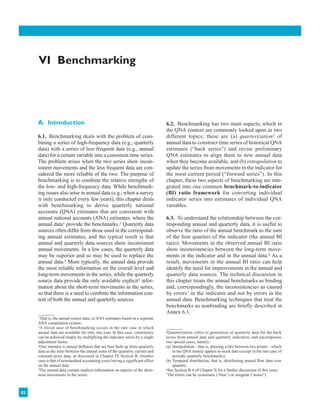
  • 5. VI BENCHMARKING 86 Chart 6.1. Pro Rata Distribution and the Step Problem The Indicator and the Derived Benchmarked QNA Estimates In this example, the step problem shows up as an increase in the derived series from q4 1998 to q1 1999 that is not matched by the move- ments in the source data.The quarterized data erroneously show a quarter-to-quarter rate of change for the first quarter of 1999 of 1.5% while the corresponding rate of change in source data is –1.8% (in this series, the first quarter is always relatively low because of seasonal factors). Benchmark-to-Indicator Ratio It is easier to recognize the step problem from charts of the BI ratio,where it shows up as abrupt upward or downward steps in the BI ratios between q4 of one year and q1 of the next year. In this example, the step problem shows up as a large upward jump in the BI ratio from q4 1998 to q1 1999. 1998 1999 2000 Indicator (left-hand scale) QNA estimates derived using pro rata distribution (right-hand scale) Back Series Forward Series (The corresponding data are given in Example 6.1) 96 98 100 102 104 106 108 960 980 1,000 1,020 1,040 1,060 1,080 9.8 9.9 10.0 10.1 10.2 10.3 10.4 10.5 1998 1999 2000
  • 6. scaling up or down the indicator (Iq,β +1) by the BI ratio for the last quarter of the last benchmark year (X4,β /I4,β ). 6.20. Also, note that if the quarterly estimates for the last benchmark year X4,β were derived using the pro rata technique in equation (6.1), for all quarters, the implied quarterly BI ratios are identical and equal to the annual BI ratio. That is, it follows from equation (6.1) that (X4,β/I4,β) = (Xq,β/Iq,β) = (Aβ/Σq Iq,β).17 6.21. Thus, as shown in equations (6.1) and (6.2), distribution refers to constructing the back series by using the BI ratio for the current year as adjust- ment factors to scale up or down the QNA source data, while extrapolation refers to constructing the forward series by carrying that BI ratio forward. C. The Proportional Denton Method 1. Introduction 6.22. The basic distribution technique shown in the previous section introduced a step in the series, and thus distorted quarterly patterns, by making all adjustments to quarterly growth rates to the first quarter. This step was caused by suddenly chang- ing from one BI ratio to another. To avoid this dis- tortion, the (implicit) quarterly BI ratios should change smoothly from one quarter to the next, while averaging to the annual BI ratios.18 Consequently, all quarterly growth rates will be adjusted by gradually changing, but relatively similar, amounts. 2. The Basic Version of the Proportional Denton Method 6.23. The basic version of the proportional Denton benchmarking technique keeps the benchmarked series as proportional to the indicator as possible by minimizing (in a least-squares sense) the difference in relative adjustment to neighboring quarters sub- ject to the constraints provided by the annual benchmarks. A numerical illustration of its opera- tion is shown in Example 6.2 and Chart 6.2. 6.24. Mathematically, the basic version of the pro- portional Denton technique can be expressed as19 (6.3) under the restriction that, for flow series,20 . That is, the sum21of the quarters should be equal to the annual data for each benchmark year,22 where t is time (e.g., t = 4y – 3 is the first quarter of year y, and t = 4y is the fourth quarter of year y); Xt is the derived QNA estimate for quarter t; It is the level of the indicator for quarter t; Ay is the annual data for year y; β is the last year for which an annual benchmark is available; and T is the last quarter for which quarterly source data are available. X A y t t T y = ∑ = ∈{ } 2 1 , .....β min – ,... ,... ..., ,...... – – 1 4 1 1 2 2 1 4 X X X t t t t t T T X I X I t T β β ( ) =       ∈ ( ) { } ∑ The Proportional Denton Method 87 17Thus, in this case, it does not matter which period is being moved. Moving from (a) the fourth quarter of the last benchmark year, (b) the average of the last benchmark year, or (c) the same quarter of the last benchmark year in proportion to the movements in the indi- cator from the corresponding periods gives the same results. Formally, it follows from equation (6.1) that 18In the standard case of binding annual benchmarks. q q q q q q q q X X I I X I I A I I , , , , , , , , , β β β β β β β β β β + + + + = ⋅       = ⋅       = ⋅         ∑ 1 4 1 4 1 1 19This presentation deviates from Denton’s original proposal by omit- ting the requirement that the value for the first period be predeter- mined.As pointed out by Cholette (1984), requiring that the values for the first period be predetermined implies minimizing the first correc- tion and can in some circumstances cause distortions to the bench- marked series. Also, Denton’s original proposal dealt only with estimating the back series. 20For the less common case of stock series, the equivalent constraint is that the value of the stock at the end of the final quarter of the year is equal to the stock at the end of the year. For index number series, the con- straint can be formulated as requiring the annual average of the quarters to be equal to the annual index or the sum of the quarters to be equal to four times the annual index. The two expressions are equivalent. 21Applies also to flow series in which the indicator is expressed as index numbers; the annual total of the indicator should still be expressed as the sum of the quarterly data. 22Theannualbenchmarksmaybeomittedforsomeyearstoallowforcases in which independent annual source data are not available for all years.
  • 7. 6.25. The proportional Denton technique implicitly constructs from the annual observed BI ratios a time series of quarterly benchmarked QNA estimates-to- indicator (quarterly BI) ratios that is as smooth as possible and, in the case of flow series: • For the back series, (y {1,...β}) averages23 to the annual BI ratios for each year y. • For the forward series, (y {β + 1.....}) are kept constant and equal to the ratio for the last quarter of the last benchmark year. We will use this interpretation of the proportional Denton method to develop an enhanced version in the next section. 6.26. The proportional Denton technique, as pre- sented in equation (6.3), requires that the indicator contain positive values only. For series that contain zeroes but not negative values, this problem can be circumvented by simply replacing the zeroes with values infinitesimally close to zero. For series that can take both negative and positive values, and are derived as differences between two non-negative series, such as changes in inventories, the problem can be avoided by applying the proportional Denton method to the opening and closing inventory levels rather than to the change. Alternatively, the problem can be circumvented by temporarily turning the indi- cator into a series containing only positive values by adding a sufficiently large constant to all periods, benchmarking the resulting indicator using equation (6.3), and subsequently deducting the constant from the resulting estimates. 6.27. For the back series, the proportional Denton method results in QNA quarter-to-quarter growth rates that differ from those in the indicator (e.g., see VI BENCHMARKING 88 Example 6.2. The Proportional Denton Method Same data as in Example 6.1. Indicator Estimated The Period-to-Period Annual Annual BI Derived QNA Quarterly Period-to-Period Indicator Rate of Change Data Ratios Estimates BI ratios Rate of Change q1 1998 98.2 969.8 9.876 q2 1998 100.8 2.6% 998.4 9.905 3.0% q3 1998 102.2 1.4% 1,018.3 9.964 2.0% q4 1998 100.8 –1.4% 1,013.4 10.054 –0.5% Sum 402.0 4000.0 9.950 4,000.0 q1 1999 99.0 –1.8% 1,007.2 10.174 –0.6% q2 1999 101.6 2.6% 1,042.9 10.264 3.5% q3 1999 102.7 1.1% 1,060.3 10.325 1.7% q4 1999 101.5 –1.2% 1,051.0 10.355 –0.9% Sum 404.8 0.7% 4161.4 10.280 4,161.4 4.0% q1 2000 100.5 –1.0% 1,040.6 10.355 –1.0% q2 2000 103.0 2.5% 1,066.5 10.355 2.5% q3 2000 103.5 0.5% 1,071.7 10.355 0.5% q4 2000 101.5 –1.9% 1,051.0 10.355 –1.9% Sum 408.5 0.9% ? ? 4,229.8 1.6% BI Ratios • For the back series (1998–1999): In contrast to the pro rata distribution method in which the estimated quarterly BI ratio jumped abruptly from 9.950 to 10.280, the proportional Denton method produces a smooth series of quarterly BI ratios in which: The quarterly estimates sum to 4000, that is, the weighted average BI ratio for 1998 is 9.950. The quarterly estimates sum to 4161.4, that is, the weighted average for 1999 is equal to 1.0280. The estimated quarterly BI ratio is increasing through 1998 and 1999 to match the increase in the observed annual BI ratio.The increase is smallest at the beginning of 1998 and at the end of 1999. • For the forward series (2000),the estimates are obtained by carrying forward the quarterly BI ratio (10.355) for the last quarter of 1999 (the last benchmark year). Rates of Change • For the back series,the quarterly percentage changes in 1998 and 1999 are adjusted upwards for all quarters to match the higher rate of change in the annual data. • For the forward series, the quarterly percentage changes in 1999 are identical to those of the indicator; but note that the rate of change from 1999 to 2000 in the derived QNA series (1.6%) is higher than the annual rate of change in the indicator (0.9%).The next section provides an extension of the method that can be use to ensure that annual rate of change in the derived QNA series equals the annual rate of change in the indicator, if that is desired. (These results are illustrated in Chart 6.2.) 23annual weighted average where the weights are q y q y q y q w I I , , , = = ∑ 1 4 X I w A I q y q y q y y q y q q , , , , ⋅ =       = = ∑ ∑ 1 4 1 4
  • 8. Example 6.2). In extreme cases, the method may even introduce new turning points in the derived series or change the timing of turning points; however, these changes are a necessary and desirable result of incor- porating the information contained in the annual data. 6.28. For the forward series, the proportional Denton method results in quarter-to-quarter growth rates that are identical to those in the indicator but also in an annual growth rate for the first year of the forward series that differs from the corresponding growth rate of the source data (see Example 6.2). This difference in the annual growth rate is caused by the way the indicator is linked in. By carrying forward the quar- terly BI ratio for the last quarter of the last benchmark year, the proportional Denton method implicitly “forecasts” the next annual BI ratio as different from the last observed annual BI ratio, and equal to the The Proportional Denton Method 89 Chart 6.2. Solution to the Step Problem:The Proportional Denton Method The Indicator and the Derived Benchmarked QNA Estimates Benchmark-to-Indicator Ratios 960 980 1000 1020 1040 1060 1080 96 98 100 102 104 106 108 1998 1999 2000 Indicator (left-hand scale) QNA estimates derived using pro rata distribution (right-hand scale) 1998–99 distributed 2000 extrapolated using Proportional Denton (right-hand scale) Back Series Forward Series (The corresponding data are given in Example 6.2) 1998 1999 2000 9.8 9.9 10.0 10.1 10.2 10.3 10.4 10.5 Annual step change 1998–99 distributed 2000 extrapolated using Proportional Denton
  • 9. quarterly BI ratio for the last quarter of the last benchmark year. As explained in Annex 6.2, the pro- portional Denton method will result in the following: • It will partly adjust for any systematic bias in the indicator’s annual rate of change if the bias is suf- ficiently large relative to any amount of noise, and thus, on average, lead to smaller revisions in the QNA estimates. • It will create a wagging tail effect with, on average, larger revisions if the amount of noise is suffi- ciently large relative to any systematic bias in the annual growth rate of the indicator. The next section presents an enhancement to the basic proportional Denton that better incorporates information on bias versus noise in the indicator’s movements. 6.29. For the forward series, the basic proportional Denton method implies moving from the fourth quarter of the last benchmark year (see equation (6.2.a)). As shown in Annex 6.2, other possible start- ing points may cause a forward step problem, if used together with benchmarking methods for the back series that avoid the step problem associated with pro rata distribution: • Using growth rates from four quarters earlier. Effectively, the estimated quarterly BI ratio is fore- cast as the same as four quarters earlier. This method maintains the percentage change in the indicator over the previous four quarters but it does not maintain the quarterly growth rates, disregards the information in past trends in the annual BI ratio, and introduces potential sever steps between the back series and the forward series. • Using growth rates from the last annual average. Effectively, the estimated quarterly BI ratio is fore- cast as the same as the last annual BI ratio. This method results in annual growth rates that equal those in the indicator; however, it also disregards the information in past trends in the annual BI ratio and introduces an unintended step between the back series and the forward series. 6.30. When the annual data later become available, the extrapolated QNA data would need to be re-esti- mated. As a result of the benchmarking process, new data for one year will also lead to changes in the quar- terly movements for the preceding year(s). This effect occurs because the adjustment for the errors in the indicator is distributed smoothly over several quarters, not just within the same year. For example, as illustrated in Example 6.3 and Chart 6.3, if the 1999 annual data subsequently showed that the downward error in the indicator for 1998 for Example 6.2 was reversed, then • the 1999 QNA estimates would be revised down; • the estimates in the second half of 1998 would be revised down (to smoothly adjust to the 1999 val- ues); and • the estimates in the first half of 1998 would need to be revised up (to make sure that the sum of the four quarters was still consistent with the 1998 annual total). While these effects may be complex, it should be emphasized that they are an inevitable and desired implication of incorporating the information pro- vided by the annual data concerning the errors in the long-term movements of the quarterly indicator. 3. Enhancements to the Proportional Denton Method for Extrapolation 6.31. It is possible to improve the estimates for the most recent quarters (the forward series) and reduce the size of later revisions by incorporating informa- tion on past systematic movements in the annual BI ratio. It is important to improve the estimates for these quarters, because they are typically of the keen- est interest to users. Carrying forward the quarterly BI ratio from the last quarter of the last year is an implicit forecast of the annual BI ratio, but a better forecast can usually be made. Accordingly, the basic Denton technique can be enhanced by adding a fore- cast of the next annual BI ratio, as follows: • If the annual growth rate of the indicator is system- atically biased compared to the annual data,24 then, on average, the best forecast of the next year’s BI ratio is the previous year’s value multiplied by the average relative change in the BI ratio. • If the annual growth rate of the indicator is unbi- ased compared to the annual data (i.e., the annual BI follows a random walk process), then, on aver- age, the best forecast of the next year’s BI ratio is the previous annual value. VI BENCHMARKING 90 24The indicator’s annual growth rate is systematically biased if the ratio between (a) the ratio of annual of change in the indicator and (b) the ratio of annual change in the annual data on average is signifi- cantly different from one or, equivalently, that the ratio of annual change in the annual BI ratio on average is significantly different from one, as seen from the following expression: A A I I A I A I BI BI y y q y q q y q y q y q y q y q y y – , , – , – , – – 1 1 4 1 1 4 1 4 1 1 1 4 1 = = = = ∑ ∑ ∑ ∑ = =
  • 10. • If the annual BI is fluctuating symmetrically around its mean, on average, the best forecast of the next year’s BI ratio is the long-term average BI value. • If the movements in the annual BI ratio are follow- ing a stable, predictable time-series model (i.e., an ARIMA25 orARMA26 model) then, on average, the best forecast of the next year’s BI ratio may be obtained from that model. • If the fluctuations in the annual BI ratio are corre- lated with the business cycle27 (e.g., as manifested in the indicator), then, on average, the best forecast of the next year’s BI ratio may be obtained by modeling that correlation. The Proportional Denton Method 91 Example 6.3. Revisions to the Benchmarked QNA Estimates Resulting from Annual Benchmarks for a NewYear This example is an extension of Example 6.2 and illustrates the impact on the back series of incorporating annual data for a new year,and sub- sequent revisions to the annual data for that year. Assume that preliminary annual data for 2000 become available and the estimate is equal to 4,100.0 (annual data A). Later on, the preliminary estimate for 2000 is revised upwards to 4,210.0 (annual data B). Using the equation presented in (6.3) to distribute the annual data over the quarters in proportion to the indicator will give the following sequence of revised QNA estimates: Indicator Revised QNA Estimates Quarterized BI Ratios Period-to Derived Derived Period Annual Annual Annual Annual in in The rate of Data BI Ratio Data BI Ratio Example With With Example With With Date Indicator Change 2000A 2000A 2000B 2000B 6.2 2000A 2000B 6.2 2000A 2000B q1 1998 98.2 969.8 968.1 969.5 9.876 9.858 9.873 q2 1998 100.3 2.6% 998.4 997.4 998.3 9.905 9.895 9.903 q3 1998 102.2 1.4% 1,018.3 1,018.7 1,018.4 9.964 9.967 9.965 q4 1998 100.8 –1.4% 1,013.4 1,015.9 1,013.8 10.054 10.078 10.058 Sum 402.0 4,000.0 9.950 4,000.0 9.950 q1 1999 99.0 –1.8% 1,007.2 1,012.3 1,008.0 10.174 10.225 10.182 q2 1999 101.6 2.6% 1,042.9 1,047.2 1,043.5 10.264 10.307 10.271 q3 1999 102.7 1.1% 1,060.3 1,059.9 1,060.3 10.325 10.321 10.324 q4 1999 101.5 –1.2% 1,051.0 1,042.0 1,049.6 10.355 10.266 10.341 Sum 404.8 0.7% 4,161.4 10.280 4,161.4 10.280 q1 2000 100.5 –1.0% 1,040.6 1,019.5 1,037.4 10.355 10.144 10.323 q2 2000 103.0 2.5% 1,066.5 1,035.4 1,061.8 10.355 10.052 10.308 q3 2000 103.5 0.5% 1,071.7 1,034.1 1,065.9 10.355 9.991 10.299 q4 2000 101.5 –1.9% 1,051.0 1,011.0 1,044.9 10.355 9.961 10.294 Sum 408.5 0.9% 4,100.0 10.037 4,210.0 10.306 4,229.8 4,100.0 4,210.0 As can be seen, incorporating the annual data for 2000 results in (a) revisions to both the 1999 and the 1998 QNA estimates, and (b) the estimates for one year depend on the difference in the annual movements of the indicator and the annual data for the previous years, the current year, and the following years. In case A, with an annual estimate for 2000 of 4100.0, the following can be observed: • The annual BI ratio increases from 9.950 in 1998 to 10.280 in 1999 and then drops to 10.037 in 2000. Correspondingly, the derived quarterly BI ratio increases gradually from q1 1998 through q3 1999 and then decreases through 2000. • Compared with the estimates obtained in Example 6.2, incorporating the 2000 annual estimate resulted in the following revisions to the path of the quar- terly BI ratio through 1998 and 1999: To smooth the transition to the decreasing BI ratios through 2000, which are caused by the drop in the annual BI ratio from 1999 to 2000, the BI ratios for q3 and q4 of 1999 have been revised downwards. The revisions downward of the BI ratios for q3 and q4 of 1999 is matched by an upward revision to the BI ratios for q1 and q2 of 1999 to ensure that the weighted average of the quarterly BI ratios for 1999 is equal to the annual BI ratio for 1999. To smooth the transition to the new BI ratios for 1999, the BI ratios for q3 and q4 of 1998 have been revised upward; consequently, the BI ratios for q1 and q2 of 1998 have been revised downwards. • As a consequence a turning point in the new time series of quarterly BI ratios has been introduced between the third and the fourth quarter of 1999, in contrast to the old BI ratio time series, which increased during the whole of 1999. In case B, with an annual estimate for 2000 of 4210.0, the following can be observed: • The annual BI ratio for 1999 of 10.306 is slightly higher than the 1999 ratio of 10.280, but: The ratio is lower than the initial q4 1999 BI ratio of 10.325 that was carried forward in Example 6.2 to obtain the initial quarterly estimates for 2000. Correspondingly, the initial annual estimate for 2000 obtained in Example 6.2 was higher than the new annual estimate for 2000. • Consequently, compared with the initial estimates from Example 6.2, the BI ratios have been revised downwards from q3 1999 onwards. • In spite of the fact that the annual BI ratio is increasing, the quarterized BI ratio is decreasing during 2000.This is caused by the steep increase in the quar- terly BI ratio during 1999 that was caused by the steep increase in the annual BI ratio from 1998 to 2000. (These results are illustrated in Chart 6.3.) 27Lags in incorporating deaths and births of businesses in quarterly sample frames may typically generate such correlations. 25Autoregressive integrated moving average time-series models. 26Autoregressive moving average time-series models.
  • 11. Note that only the annual BI ratio and not the annual benchmark value has to be forecast, and the BI ratio is typically easier to forecast than the annual bench- mark value itself. 6.32. To produce a series of estimated quarterly BI ratios taking into account the forecast, the same prin- ciples of least-square minimization used in the Denton formula can also be used with a series of annual BI ratios that include the forecast. Since the benchmark values are not available, the annual con- straint is that the weighted average of estimated quar- terly BI ratios is the same as the corresponding observed or forecast annual BI ratios and that period- to-period change in the time series of quarterly BI ratios is minimized. VI BENCHMARKING 92 Chart 6.3. Revisions to the Benchmarked QNA Estimates Resulting from Annual Benchmarks for a NewYear Benchmark-to-Indicator Ratios 960 980 1000 1020 1040 1060 1080 96 98 100 102 104 106 108 1998 1999 2000 Indicator (left-hand scale) With 2000A (right-hand scale) With 2000B (right-hand scale) Back Series Forward Series (The corresponding data are given in Example 6.3) 1998–99 distributed 2000 extrapolated using Proportional Denton (right-hand scale) 1998 1999 2000 With 2000A With 2000B 1998–99 distributed 2000 extrapolated using Proportional Denton 9.8 9.9 10.0 10.1 10.2 10.3 10.4 10.5
  • 12. 6.33. In mathematical terms: (6.4.a) under the restriction that (a) and (b) Where , and where QBIt is the estimated quarterly BI ratio (Xt /It) for period t; ABIy is the observed annual BI ratio (At/Σq Iq,y) for year y {1,...β}; and ÂBIy is the forecast annual BI ratio for year y {β + 1.....}. 6.34. Once a series of quarterly BI ratios is derived, the QNA estimate can be obtained by multiplying the indicator by the estimated BI ratio. Xt = QBIt • It (6.4.b) 6.35. The following shortcut version of the enhanced Denton extrapolation method gives similar results for less volatile series. In a computerized system, the shortcut is unnecessary, but it is easier to follow in an example (see Example 6.4 and Chart 6.4). This method can be expressed mathematically as (a) Q̂BI2,β = QBI2,β + 1/4 • η (6.5) Q̂BI3,β = QBI3,β + 1/4 • η Q̂BI4,β = QBI4,β – 1/2 • η (b) Q̂BI1,β + 1 = Q̂BI4,β – η Q̂BIq,β + 1 = Q̂BIq – 1,β + 1 – η where η = 1/3(QBI4,β – ÂBIβ + 1) (a fixed parameter for adjustments that ensures that the estimated quar- terly BI ratios average to the correct annual BI ratios); QBIq,β is the original BI ratio estimated for quarter q of the last benchmark year; Q̂BIq,β is the adjusted BI ratio estimated for quarter q of the last benchmark year; Q̂BIq,β+1 is the forecast BI ratio for quarter q of the fol- lowing year; and ÂBIβ + 1 is the forecast average annual BI ratio for the following year. 6.36. While national accountants are usually reluc- tant to make forecasts, all possible methods are based on either explicit or implicit forecasts, and implicit forecasts are more likely to be wrong because they are not scrutinized. Of course, it is often the case that the evidence is inconclusive, so the best forecast is simply to repeat the last observed annual BI ratio. D. Particular Issues 1. Fixed Coefficient Assumptions 6.37. In national accounts compilation, potential step problems may arise in cases that may not always be thought of as a benchmark-indicator relationship. One important example is the frequent use of assumptions of fixed coefficients relating inputs (total or part of intermediate consumption or inputs of labor and/or capital) to output (“IO ratios”). Fixed IO ratios can be seen as a kind of a benchmark-indicator relationship, where the available series is the indicator for the miss- ing one and the IO ratio (or its inverse) is the BI ratio. If IO ratios are changing from year to year but are kept constant within each year, a step problem is created. Accordingly, the Denton technique can be used to generate smooth time series of quarterly IO ratios based on annual (or less frequent) IO coefficients. Furthermore, systematic trends can be identified to forecast IO ratios for the most recent quarters. 2. Within-Year Cyclical Variations in Coefficients 6.38. Another issue associated with fixed coefficients is that coefficients that are assumed to be fixed may in fact be subject to cyclical variations within the year. IO ratios may vary cyclically owing to inputs that do not w I I t t t t t y y = ∈ ( ) { } = ∑ 4 3 4 1 4 – ,... for β QBI w ABI t y t t y y t y ⋅ = ∈ ( ) { } ∈ + { } = + ∑ 4 3 4 4 1 4 1 – – ˆ ...... , ,.... . for T β β QBI w ABI t y t t y y t y ⋅ = ∈ ( ) { } ∈{ } = ∑ 4 3 4 1 4 1 – ,... , ,... . for β β min – ,... ,.... ...., ,....... – 1 4 1 2 2 1 4 QBI QBI QBI t t t T T QBI QBI t T β β ( ) = [ ] ∈ ( ) { } ∑ Particular Issues 93
  • 13. vary proportionately with output, typically fixed costs such as labor, capital, or overhead such as heating and cooling. Similarly, the ratio between income flows (e.g., dividends) and their related indicators (e.g., prof- its) may vary cyclically. In some cases, these variations may be according to a seasonal pattern and be known.28 It should be noted that omitted seasonal variations are only a problem in the original non-seasonally adjusted data, as the variations are removed in seasonal adjust- ment and do not restrict the ability to pick trends and turning points in the economy. However, misguided attempts to correct the problem in the original data could distort the underlying trends. 6.39. To incorporate a seasonal pattern on the target QNA variable, without introducing steps in the series, one of the following two procedures can be used: (a) BI ratio-based procedure Augment the benchmarking procedure as out- lined in equation (6.4) by incorporating the a pri- ori assumed seasonal variations in the estimated quarterly BI ratios as follows: (6.6) under the same restrictions as in equation (6.4), where SFt is a time series with a priori assumed seasonal factors. min – ,... ,.... ...., ,....... – – 1 4 1 1 2 2 1 4 QBI QBI QBI QBI SF QBI SF t T t t t t t T β β ( ) =       ∈ ( ) { } ∑ T VI BENCHMARKING 94 28Cyclical variations in assumed fixed coefficients may also occur because of variations in the business cycle. These variations cause serious errors because they may distort trends and turning points in the economy. They can only be solved by direct measurement of the target variables. Example 6.4. Extrapolation Using Forecast BI Ratios Same data as Examples 6.1 and 6.3 Original estimates Quarter to quarter rates of change from Example 6.2 Original QNA Extrapolation using Estimates Annual estimates forecast BI ratios from Based on Annual BI BI for Forecast Original Example forecast Date Indicator data ratios ratios 1997–1998 BI ratio Estimate indicator 6.2 BI ratios q1 1998 98.2 9.876 969.8 q2 1998 100.8 9.905 998.4 2.60% 3.00% 3.00% q3 1998 102.2 9.964 1,018.3 1.40% 2.00% 2.00% q4 1998 100.8 10.054 1,013.4 –1.40% –0.50% –0.50% Sum 402.0 4,000.0 9.950 4,000.0 q1 1999 99.0 10.174 1,007.2 –1.80% –0.60% –0.60% q2 1999 101.6 10.264 1,042.9 10.253 1,041.7 2.60% 3.50% 3.40% q3 1999 102.7 10.325 1,060.3 10.314 1,059.2 1.10% 1.70% 1.70% q4 1999 101.5 10.355 1,051 10.376 1,053.2 –1.20% –0.90% –0.20% Sum 404.8 4,161.4 10.280 4,161.4 10.280 4,161.4 0.70% 4.00% 4.00% q1 2000 100.5 10.355 1,040.6 10.42 1,047.2 –1.00% –1.00% –0.60% q2 2000 103 10.355 1,066.5 10.464 1,077.8 2.50% 2.50% 2.90% q3 2000 103.5 10.355 1,071.7 10.508 1,087.5 0.50% 0.50% 0.90% q4 2000 101.5 10.355 1,051 10.551 1,071 –1.90% –1.90% –1.50% Sum 408.5 10.355 4,229.8 10.486 4,283.5 0.90% 1.60% 2.90% This example assumes that, based on a study of movements in the annual BI ratios for a number of years, it is established that the indicator on average under- states the annual rate of growth by 2.0%. The forecast annual and adjusted quarterly BI ratios are derived as follows: The annual BI ratio for 2000 is forecast to rise to 10.486, (i.e., 10.280 • 1.02). The adjustment factor (η) is derived as –0.044, (i.e., 1/3 • (10.355 – 10.486). q2 1999: 10.253 = 10.264 + 1/4 • (–0.044) q3 1999: 10.314 = 10.325 + 1/4 • (–0.044) q4 1999: 10.376 = 10.355 – 1/2 • (–0.044) q1 2000: 10.420 = 10.376 – (–0.044) q2 2000: 10.464 = 10.420 – (–0.044) q3 2000: 10.508 = 10.464 – (–0.044) q4 2000: 10.551 = 10.508 – (–0.044) Note that for the sum of the quarters, the annual BI ratios are as measured (1999) or forecast (2000), and the estimated quarterly BI ratios move in a smooth way to achieve those annual results, minimizing the proportional changes to the quarterly indicators. (These results are illustrated in Chart 6.4.)
  • 14. (b) Seasonal adjustment-based procedure (i) Use a standard seasonal adjustment package to seasonally adjust the indirect indicator. (ii) Multiply the seasonally adjusted indicator by the known seasonal coefficients. (iii) Benchmark the resulting series to the corre- sponding annual data. 6.40. The following inappropriate procedure is sometimes used to incorporate a seasonal pattern when the indicator and the target variable have dif- ferent and known seasonal patterns: (a) distribute the annual data for one year in propor- tion to the assumed seasonal pattern of the series, and (b) use the movements from the same period in the previous year in the indicator to update the series. 6.41. This procedure preserves the superimposed seasonal patterns when used for one year only. When Particular Issues 95 Chart 6.4. Extrapolation Using Forecast BI Ratios Benchmark-to-Indicator Ratios 960 980 1000 1020 1040 1060 1080 96 98 100 102 104 106 108 1998 1999 2000 Indicator (left-hand scale) 1998–99 distributed 2000 extrapolated using Proportional Denton (right-hand scale) Extrapolating using forcasted BI ratios (right-hand scale) Back Series Forward Series (The corresponding data are given in Example 6.4) 1998 1999 2000 Extrapolating using forcasted BI ratios 1998–99 distributed 2000 extrapolated using Proportional Denton 9.8 10.0 10.2 10.4 10.6
  • 15. the QNA estimates are benchmarked, however, this procedure will introduce breaks in the series that can remove or distort trends in the series and introduce more severe errors than those that it aims to prevent (see Annex 6.2 for an illustration). 3. Benchmarking and Compilation Procedures 6.42. Benchmarking should be an integral part of the compilation process and should be conducted at the most detailed compilation level. In practice, this may imply benchmarking different series in stages, where data for some series, which have already been bench- marked, are used to estimate other series, followed by a second or third round of benchmarking. The actual arrangements will vary depending on the particulari- ties of each case. 6.43. As an illustration, annual data may be available for all products, but quarterly data are available only for the main products. If it is decided to use the sum of the quarterly data as an indicator for the other products, the ideal procedure would be first to bench- mark each of the products for which quarterly data are available to the annual data for that product, and then to benchmark the quarterly sum of the bench- marked estimates for the main products to the total. Of course, if all products were moving in similar ways, this would give similar results to directly benchmarking the quarterly total to the annual total. 6.44. In other cases, a second or third round of benchmarking may be avoided and compilation pro- cedure simplified. For instance, a current price indi- cator can be constructed as the product of a quantity indicator and a price indicator without first bench- marking the quantity and price indicators to any cor- responding annual benchmarks. Similarly, a constant price indicator can be constructed as a current price indicator divided by a price indicator without first benchmarking the current price indicator. Also, if output at constant prices is used as an indicator for intermediate consumption, the (unbenchmarked) constant price output indicator can be benchmarked to the annual intermediate consumption data directly. It can be shown that the result is identical to first benchmarking the output indicator to annual output data, and then benchmarking the resulting bench- marked output estimates to the annual intermediate consumption data. 6.45. To derive quarterly constant price data by deflating current price data, the correct procedure would be first to benchmark the quarterly current price indicator and then to deflate the benchmarked quarterly current price data. If the same price indices are used in the annual and quarterly accounts, the sum of the four quarters of constant price data should be taken as the annual estimate, and a second round of benchmarking is unnecessary. As explained in Chapter IX Section B, annual deflators constructed as unweighted averages of monthly or quarterly price data can introduce an aggregation over time error in the annual deflators and subsequently in the annual constant price data that can be significant if there is quarterly volatility. Moreover, if, in those cases, quar- terly constant price data are derived by benchmarking a quarterly constant price indicator derived by deflat- ing the current price indicator to the annual constant price data, the aggregation over time error will be passed on to the implicit quarterly deflator, which will differ from the original price indices. Thus, in those cases, annual constant price data should in prin- ciple be derived as the sum of quarterly or even monthly deflated data if possible. If quarterly volatil- ity is insignificant, however, annual constant price estimates can be derived by deflating directly and then benchmarking the quarterly constant price esti- mates to the annual constant price estimates. 4. Balancing Items and Accounting Identities 6.46. The benchmarking methods discussed in this chapter treat each time series as an independent vari- able and thus do not take into account any accounting relationship between related time series. Consequently, the benchmarked quarterly time series will not auto- matically form a consistent set of accounts. For exam- ple, quarterly GDP from the production side may differ from quarterly GDP from the expenditure side, even though the annual data are consistent. The annual sum of these discrepancies, however, will cancel out for years where the annual benchmark data are balanced.29 While multivariate benchmarking methods exist that take the relationship between the time series as an additional constraint, they are too complex and demanding to be used in QNA. 6.47. In practice, the discrepancies in the accounts can be minimized by benchmarking the different parts of the accounts at the most detailed level and building aggregates from the benchmarked compo- nents. If the remaining discrepancies between, for VI BENCHMARKING 96 29The within-year discrepancies will in most cases be relatively insignificant for the back series.
  • 16. instance, GDP from the production and expenditure side are sufficiently small,30 it may be defensible to distribute them proportionally over the correspond- ing components on one or both sides. In other cases, it may be best to leave them as explicit statistical dis- crepancies, unless the series causing these discrepan- cies can be identified. Large remaining discrepancies indicate that there are large inconsistencies between the short-term movements for some of the series. 5. More Benchmarking Options 6.48. The basic version of the proportional Denton technique presented in equation (6.3) can be expanded by allowing for alternative benchmark options, as in the following examples: • The annual benchmarks may be omitted for some years to allow for cases where independent annual source data are not available for all years. • Sub-annual benchmarks may be specified by requiring that the values of the derived series are equal to some predetermined values in certain benchmark quarters; or the half-yearly sums of the derived quarterly estimates are equal to half-yearly benchmark data for some periods. • Benchmarks may be treated as nonbinding. • Quarters that are known to be systematically more error prone than others may be adjusted relatively more than others. The formulas for the two latter extensions are pro- vided in Section B.2 of Annex 6.1. 6. Benchmarking and Revisions 6.49. To avoid introducing distortions in the series, incorporation of new annual data for one year will gen- erally require revision of previously published quar- terly data for several years. This is a basic feature of all acceptable benchmarking methods. As explained in paragraph 6.30, and as illustrated in Example 6.3, in addition to the QNA estimates for the year for which new annual data are to be incorporated, the quarterly data for one or several preceding and following years, may have to be revised. In principle, previously pub- lished QNA estimates for all preceding and following years may have to be adjusted to maximally preserve the short-term movements in the indicator, if the errors in the indicator are large. In practice, however, with most benchmarking methods, the impact of new annual data will gradually be diminishing and zero for sufficiently distant periods. 6.50. One of the advantages of the Denton method compared with several of the alternative methods discussed in Annex 6.1, is that it allows for revi- sions to as many preceding years as desired. If desired, revisions to some previously published QNA estimates can be avoided by specifying those estimates as “quarterly benchmark restrictions.” This option freezes the values for those periods, and thus can be used to reduce the number of years that have to be revised each time new annual data become available. To avoid introducing significant distortions to the benchmarked series, however, at least two to three years preceding (and following) years should be allowed to be revised each time new annual data become available. In general, the impact on more distant years will be negligible. 7. Other Comments 6.51. Sophisticated benchmarking techniques use advanced concepts. In practice, however, they require little time or concern in routine quarterly compilation. In the initial establishment phase, the issues need to be understood and the processes automated as an integral part of the QNA production system. Thereafter, the techniques will improve the data and reduce future revisions without demanding time and attention of the QNA compiler. It is good practice to check the new benchmarks as they arrive each year in order to replace the previous BI ratio forecasts and make new annual BI forecasts. A useful tool for doing so is a table of observed annual BI ratios over the past several years. It will be usual for the BI ratio forecasts to have been wrong to varying degrees, but the important question is whether the error reveals a pattern that would allow better forecasts to be made in the future. In addition, changes in the annual BI ratio point to issues concerning the indicator that will be of rele- vance to the data suppliers. Particular Issues 97 30That is, so that the impact on the growth rates are negligible.
  • 17. Annex 6.1. Alternative Benchmarking Methods 98 A. Introduction 6.A1.1. There are two main approaches to bench- marking of time series: a purely numerical approach and a statistical modeling approach. The numerical differs from the statistical modeling approach by not specifying a statistical time-series model that the series is assumed to follow. The numerical approach encompasses the family of least-squares minimization methods proposed by Denton (1971) and others,1 the Bassie method,2 and the method proposed by Ginsburgh (1973). The modeling approach encompasses ARIMA3 model-based methods proposed by Hillmer and Trabelsi (1987), State Space models proposed by Durbin and Quenneville (1997), and a set of regression models proposed by various Statistics Canada staff.4 In addition, Chow and Lin (1971) have proposed a multivariable general least-squares regression approach for interpolation, distribution, and extrap- olation of time series. While not a benchmarking method in a strict sense, the Chow-Lin method is related to the statistical approach, particularly to Statistics Canada’s regression models. 6.A1.2. The aim of this annex is to provide a brief review, in the context of compiling quarterly national accounts (QNA), of the most familiar of these methods and to compare them with the pre- ferred proportional Denton technique with enhance- ments. The annex is not intended to provide an extensive survey of all alternative benchmarking methods proposed. 6.A1.3. The enhanced proportional Denton tech- nique provides many advantages over the alterna- tives. It is, as explained in paragraph 6.7, by logical consequence optimal if the general benchmarking objective of maximal preservation of the short-term movements in the indicator is specified as keeping the quarterly estimates as proportional to the indica- tor as possible and the benchmarks are binding. In addition, compared with the alternatives, the enhanced proportional Denton technique is rela- tively simple, robust, and well suited for large-scale applications. Moreover, the implied benchmark- indicator (BI) ratio framework provides a general and integrated framework for converting indicator series into QNA estimates through interpolation, distribution, and extrapolation with an indicator that, in contrast to additive methods, is not sensitive to the overall level of the indicators and does not tend to smooth away some of the quarter-to-quarter rates of change in the data. The BI framework also encompasses the basic extrapolation with an indica- tor technique used in most countries. 6.A1.4. In contrast, the potential advantage of the various statistical modeling methods over the enhanced proportional Denton technique is that they explicitly take into account any supplementary information about the underlying error mechanism and other aspects of the stochastic properties of the series. Usually, however, this supplementary infor- mation is not available in the QNA context. Moreover, some of the statistical modeling methods render the danger of over-adjusting the series by interpreting true irregular movements that do not fit the regular patterns of the statistical model as errors, and thus removing them. In addition, the enhance- ment to the proportional Denton provided in Section D of Chapter VI allows for taking into account sup- plementary information about seasonal and other short-term variations in the BI ratio. Further enhancements that allow for incorporating any sup- plementary information that the source data for some quarters are weaker than others, and thus should be adjusted more than others, are provided in Section B.2 of this annex, together with a nonbind- ing version of the proportional Denton. 6.A1.5. Also, for the forward series, the enhance- ments to the proportional Denton method developed 1Helfand, Monsour, and Trager (1977), and Skjæveland (1985). 2Bassie (1958). 3Autoregressive integrated moving average. 4Laniel, and Fyfe (1990), and Cholette and Dagum (1994).
  • 18. in Section C.3 of Chapter VI provide more and bet- ter options for incorporating various forms of infor- mation on past systematic bias in the indicator’s movements. The various statistical modeling meth- ods typically are expressed as additive relationships between the levels of the series, not the movements, that substantially limit the possibilities for alterna- tive formulation of the existence of any bias in the indicator. The enhancements to the proportional Denton method developed in Chapter VI express systematic bias in terms of systematic behavior of the relative difference in the annual growth rate of the indicator and the annual series or, equivalently, in the annual BI ratio. This provides for a more flexible framework for adjusting for bias in the indicator. B. The Denton Family of Benchmarking Methods 1. Standard Versions of the Denton Family 6.A1.6. The Denton family of least-squares-based benchmarking methods is based on the principle of movement preservation. Several least-squares- based methods can be distinguished, depending on how the principle of movement preservation is made operationally. The principle of movement preserva- tion can be expressed as requiring that (1) the quar- ter-to-quarter growth in the adjusted quarterly series and the original quarterly series should be as similar as possible or (2) the adjustment to neighboring quarters should be as similar as possible. Within each of these two broad groups, further alternatives can be specified. The quarter-to-quarter growth can be specified as absolute growth or as rate of growth, and the absolute or the relative difference of these two expressions of quarter-to-quarter growth can be minimized. Similarly, the difference in absolute or relative adjustment of neighboring quarters can be minimized. 6.A1.7. The proportional Denton method (formula D4 below) is preferred over the other versions of the Denton method for the following three main reasons: • It is substantially easier to implement. • It results in most practical circumstances in approximately the same estimates for the back series as formula D2, D3, and D5 below. • Through the BI ratio formulation used in Chapter VI, it provides a simple and elegant framework for extrapolation using the enhanced propor- tional Denton method, which fully takes into account the existence of any systematic bias or lack thereof in the year-to-year rate of change in the indicator. • Through the BI ratio formulation used in Chapter VI, it provides a simple and elegant framework for extrapolation, which supports the understand- ing of the enhanced proportional Denton method; the Denton method fully takes into account the existence of any systematic bias or lack thereof in the year-to-year rate of change in the indicator. 6.A1.8. In mathematical terms, the following are the main versions5 of the proposed least-squares bench- marking methods:6 MinD1: (6.A1.1) Min D2: (6.A1.2) Min D3: (6.A1.3) Min D4:7 (6.A1.4) min – ..., ,.... – – 1 4 1 1 2 2 X X X t t t t t T T X I X I β ( ) =       ∑ min – ..., ,.... – – 1 4 1 1 2 2 X X X t t t t t T T X X I I β ( )       = ∑ min min min ..., ,.... – – ..., ,.... – – ..., ,.... – 1 4 1 4 1 4 1 1 1 1 1 2 2 1 1 2 2 1 X X X t t t t t T X X X t t t t t T X X X t t T T T X X I I X I X I X X β β β ( ) ( ) ( )                         ( = = ∑ ∑ = = n n n ) ) ( ) [ ] = ∑ – – 1 1 2 2 n I I t t t T min – – min – – ..., ,.... ..., ,.... 1 4 1 4 1 1 1 1 2 2 2 2 X X X t T X X X t T T T X X I I X I X I t t t t t t t t β β ( ) − = ( ) − − ( ) − ( ) [ ] ∑ − ( ) − ( ) [ ] ∑ = = Annex 6.1. Alternative Benchmarking Methods 99 5The abbreviations D1, D2, D3, and D4, were introduced by Sjöberg (1982), as part of a classification of the alternative least- squares-based methods proposed by, or inspired by, Denton (1971). D1 and D4 were proposed by Denton; D2 and D3 by Helfand, Monsour, and Trager (1977); and D5 by Skjæveland (1985). 6This presentation deviates from the original presentation by the various authors by omitting their additional requirement that the value for the first period is predetermined. Also, Denton’s original proposal only dealt with the back series. 7This is the basic version of the proportional Denton.
  • 19. Min D5: (6.A1.5) All versions are minimized under the same restric- tions, that for flow series, . That is, the sum of the quarters should be equal to the annual data for each benchmark year. 6.A1.9. The various versions of the Denton family of least-squares-based benchmarking methods have the following characteristics: • The D1 formula minimizes the differences in the absolute growth between the benchmarked series Xt and the indicator series It. It can also be seen as minimizing the absolute difference of the absolute adjustments of two neighboring quarters. • The D2 formula minimizes the logarithm of the rela- tive differences in the growth rates of the two series. Formula D2 can also be looked upon as minimizing the logarithm of the relative differences of the relative adjustments of two neighboring quarters and as the logarithm of the absolute differences in the period-to- period growth rates between the two series. • The D3 formula minimizes the absolute differences in the period-to-period growth rates between the two series. • The D4 formula minimizes the absolute differences in the relative adjustments of two neighboring quarters. • The D5 formula minimizes the relative differences in the growth rates of the two series. Formula D5 can also be looked upon as minimizing the relative differences of the relative adjustments of two neighboring quarters. 6.A1.10. While all five formulas can be used for benchmarking, only the D1 formula and the D4 for- mula have linear first-order conditions for a mini- mum and thus are the easiest to implement in practice. In practice, the D1 and D4 formulas are the only ones currently in use. 6.A.1.11. The D4 formula—the proportional Denton method—is generally preferred over the D1 formula because it preserves seasonal and other short-term fluctuations in the series better when these fluctuations are multiplicatively distributed around the trend of the series. Multiplicatively distributed short-term fluctua- tions seem to be characteristic of most seasonal macro- economic series. By the same token, it seems most reasonable to assume that the errors are generally mul- tiplicatively, and not additively, distributed, unless anything to the contrary is explicitly known. The D1 formula results in a smooth additive distribution of the errors in the indicator, in contrast to the smooth multi- plicative distribution produced by the D4 formula. Consequently, as with all additive adjustment formula- tions, the D1 formula tends to smooth away some of the quarter-to-quarter rates of change in the indicator series.As a consequence, the D1 formula can seriously disturb that aspect of the short-term movements for series that show strong short-term variations. This can occur particularly if there is a substantial difference between the level of the indicator and the target vari- able. In addition, the D1 formula may in a few instances result in negative benchmarked values for some quarters (even if all original quarterly and annual data are positive) if large negative adjustments are required for data with strong seasonal variations. 6.A1.12. The D2, D3, and D5 formulas are very sim- ilar. They are all formulated as an explicit preserva- tion of the period-to-period rate of change in the indicator series, which is the ideal objective formula- tion, according to several authors (e.g., Helfand, Monsour, and Trager 1977). Although the three for- mulas in most practical circumstances will give approximately the same estimates for the back series, the D2 formula seems slightly preferable over the other two. In contrast to D2, the D3 formula will adjust small rates of change relatively more than large rates of change, which is not an appealing prop- erty. Compared to D5, the D2 formula treats large and small rates of change symmetrically and thus will result in a smoother series of relative adjustments to the growth rates. 2. Further Expansions of the Proportional Denton Method 6.A1.13. The basic version of the proportional Denton technique (D4) presented in the chapter can be further expanded by allowing for alternative or additional benchmark restrictions, such as the following: • Adjusting relatively more quarters that are known to be systematically more error prone than others. • Treating benchmarks as nonbinding. X A y t y y y 1 4 3 4 1 = ∈{ } = ∑ – , ,...β min – min – ,... ,.... ..., ,.... – – ..., ,.... – – 1 4 1 4 1 1 2 2 1 1 2 2 1 1 1 4 X X X t t t t t T X X X t t t t t T T T X X I I X I X I t T β β β ( ) ( )             ( ) { } = = ∑ ∑ = ∈ VI BENCHMARKING 100
  • 20. 6.A1.14. The following augmented version of the basic formula allows for specifying which quarters should be adjusted more than the others: (6.A1.6) under the standard restriction that That is, the sum of the quarters should be equal to the annual data for each benchmark year. Where wqt is a set of user-specified quarterly weights that specifies which quarters should be adjusted more than the others. 6.A1.15. In equation (6.A1.6), only the relative value of the user-specified weights (wqt ) matters. The absolute differences in the relative adjustments of a pair of neighboring quarters given a weight that is high relative to the weights for the others will be smaller than for pairs given a low weight. 6.A1.16. Further augmenting the basic formula as follows, allows for treating the benchmarks as non- binding: (6.A1.7) Where way is a set of user-specified annual weights that specifies how binding the annual benchmarks should be treated. Again, only the relative value of the user-specified weights matters. Relatively high values of the annual weights specify that the benchmarks should be treated as relatively binding. C. The Bassie Method 6.A1.17. Bassie (1958) was the first to devise a method for constructing monthly and quarterly series whose short-term movements would closely reflect those of a related series while maintaining consistency with annual totals. The Bassie method was the only method described in detail in Quarterly National Accounts (OECD, 1979). However, using the Bassie method as presented in OECD (1979) can result in a step problem if data for several years are adjusted simultaneously. 6.A1.18. The Bassie method is significantly less suited for QNA compilation than the proportional Denton technique with enhancements for the follow- ing main reasons: • The proportional Denton method better preserves the short-term movements in the indicator. • The additive version of the Bassie method, as with most additive adjustment methods, tends to smooth the series and thus can seriously disturb the quar- ter-to-quarter rates of change in series that show strong short-term variations. • The multiplicative version of the Bassie method does not yield an exact correction, requiring a small amount of prorating at the end. • The proportional Denton method allows for the full time series to be adjusted simultaneously, in con- trast to the Bassie method, which operates on only two consecutive years. • The Bassie method can result in a step problem if data for several years are adjusted simultane- ously and not stepwise.8 • The proportional Denton method with enhance- ments provides a general and integrated framework for converting indicator series into QNA estimates through interpolation, distribution, and extrapola- tion with an indicator. In contrast, the Bassie method does not support extrapolation; it only addresses distribution of annual data. • The Bassie method results in a more cumbersome compilation process. 6.A1.19. The following is the standard presentation of the Bassie method, as found, among others, in OECD (1979). Two consecutive years are consid- ered. No discrepancies between the quarterly and annual data for the first year are assumed, and the (absolute or relative) difference for the second year is equal to K2. 6.A1.20. The Bassie method assumes that the cor- rection for any quarter is a function of time, Kq = f(t) and that f(t) = a + bt + ct2 + dt3. The method then stip- ulates the following four conditions: (i) The average correction in year 1 should be equal to zero: min – – – . ..., ,.... – – – 1 4 2 1 1 2 1 4 3 4 2 1 X X X q t T t t t t a y t y t y y T t y w X I X I w X A β β ( ) = = = ∑ ∑ ∑ ⋅ ⋅             X A y t t y y y = ∑ = ∈{ } 4 1 4 1 – , ,... . β min – ,... ,.... ...., ,....... – – 1 4 2 1 1 2 1 4 X X X q t T t t t t T t w X I X I t T β β ( ) = ∑ ⋅ ∈         ( ) { } Annex 6.1. Alternative Benchmarking Methods 101
  • 21. (ii) The average correction in year 2 should be equal to the annual error in year 2 (K2): (iii)At the start of year 1, the correction should be zero, so as not to disturb the relationship between the first quarter of year 1 and the fourth quarter of year 0: f(0) = 0. (iv) At the end of year 2, the correction should be nei- ther increasing nor decreasing: 6.A1.21. These four conditions allow computing the following fixed coefficients to distribute the annual error in year 2 (K2) over the four quarters of year 2 and to adjust the quarterly pattern within year 1: 6.A1.22. The difference between the annual sum of the quarterly estimates and the direct annual esti- mate in year 2 (K2) can be expressed either in an additive form or in a multiplicative form. The addi- tive form is as follows: (6.A1.8) leading to the following additive version of the Bassie adjustment method: Zq,1 = Xq,1 + 0.25 • bq • K2 (6.A1.9) Zq,2 = Xq,2 + 0.25 • cq • K2 K A Xq q 2 2 2 1 4 = = ∑ – , df dt 2 0 ( ) = . f t dt K ( ) . = ∫ 2 1 2 f t dt ( ) . = ∫ 0 0 1 VI BENCHMARKING 102 Example 6.A1.1. The Bassie Method and the Step Problem Adjustment Coefficients Implied Original Annual Rate of Adjustment Adjustment Adjusted Growth Adjustment Date Estimates Estimates Error ofYear 2 ofYear 3 Estimates Rates Ratio Year 1 q1 1,000.0 –0.0981445 990.2 0.990 q2 1,000.0 –0.1440297 985.6 –0.5% 0.986 q3 1,000.0 –0.0083008 999.2 1.4% 0.999 q4 1,000.0 0.25048828 1,025.1 2.6% 1.025 Total year 1 4,000.0 4,000.0 0.00 0.0 4,000.0 Year 2 q1 1,000.0 0.57373047 –0.0981445 1,057.4 3.2% 1.057 q2 1,000.0 0.90283203 –0.1440297 1,090.3 3.1% 1.090 q3 1,000.0 1.17911122 –0.0083008 1,117.9 2.5% 1.118 q4 1,000.0 1.34423822 0.25048828 1,134.4 1.5% 1.134 Total year 2 4,000.0 4,400.0 0.10 4.0 0.0 4,400.0 Year 3 q1 1,000.0 0.57373047 1,000.0 –11.9% 1.000 q2 1,000.0 0.90283203 1,000.0 0.0% 1.000 q3 1,000.0 1.17911122 1,000.0 0.0% 1.000 q4 1,000.0 1.34423822 1,000.0 0.0% 1.000 Total year 3 4,000.0 4,000.0 0.00 4.0 In the example, revised annual estimates for years 2 and 3 were made available at the same time. As seen, the first–round adjustment of the quarterly series to align the quarterly estimates to the annual estimate for year 2 results in an upward adjustment in the growth through year 1 and year 2 but no adjustments to year 3, leading to a break in the series between q4 of year 2 and q1 of year 3. The break introduced by the first round of adjustments is not removed in the second round of adjustments to align the series to the annual estimate for year 3. In the example, the error in year 3 is zero, and the Bassie method, applied as described above, results in no further adjustments of the data. 8This step problem can be reduced, but not removed entirely, by a reformulation of the standard presentation of the method; however, use of the Bassie method is still not advisable. To be used for year 1 To be used for year 2 b1 -0.098145 c1 0.573730 b2 -0.144030 c2 0.902832 b3 -0.008301 c3 1.179111 b4 0.250488 c4 1.344238 Sum 0.0 4.0
  • 22. where q is used as a generic symbol for quarters; Zq,y is the level of the adjusted quarterly estimate for quarter q in year 1 (y = 1) and 2 (y = 2); Xq,y is the level of the preliminary quarterly estimate for quarter q in year y; and A2 is the level of the direct annual estimate for year 2. 6.A1.23. The multiplicative form is as follows: (6.A1.10) leading to the following multiplicative version of the Bassie adjustment method: Zq,1 = Xq,1 • (1 + bq • K2) (6.A1.11) Zq,2 = Xq,2 • (1 + cq • K2) The multiplicative version of the Bassie method does not yield an exact correction, and a small amount of prorating is necessary at the end of the computation. 6.A1.24. The Bassie method only works as long as not more than one year is adjusted each time and the quarterly estimates represent a continuous time series. In particular, it should be noted that (contrary to what is stated in Quarterly National Accounts (OECD 1979, page 30), when several years are to be adjusted, the process cannot be directly “continued for years 2 and 3, years 3 and 4, etc., applying the correction factors for the ‘first year’to year 2 (which has already been corrected once) and the correction factors for ‘the second year’ for year 3, and 4, etc.” That is, the following generalized version of the multiplicative Bassie method does not work: Zq,y = Xq,y • (1 + cq • Ky) • (1 + bq • Ky + 1) (6.A1.12) 6.A1.25. Example 6.A1.1, using the multiplicative version of the Bassie method, illustrates the working of the Bassie method as described in OECD (1979) and the step problem inherent in this version of the method when used for adjusting several years simultaneously. 6.A1.26. The break introduced by the use of the Bassie method, as applied above, is caused by the fact that the quarterly time series used in aligning the series to year 3 is not continuous. The time series used consists of the original data for year 3 and the data for year 2 aligned or benchmarked to the annual data for year 2. This dis- continuity is carried over into the revised series. D. The Ginsburgh-Nasse Method 6.A1.27. Ginsburgh proposed a three-step method for distribution of annual data using a related quarterly series. He did not address the problem of extrapolation, or estimation of the forward series. By slightly refor- mulating the original presentation of the method along the lines suggested by Ginsburgh himself, however, the basic version of the QNA “regression-based” compila- tion system,9 as originally formulated by Nasse (1973), for estimating both the back and the forward series emerges. In this section the following is shown: • The Ginsburgh-Nasse method is in essence identi- cal to the additive Denton (D1) method with a prior adjustment of the indicator for any significant aver- age difference between the level of the indicator and the target variable. • For both the back and forward series, the Ginsburgh-Nasse method and the D1 method with prior level adjustment result in identical estimates. • The regression component of the Ginsburgh-Nasse method constitutes an unnecessarily complicated and cumbersome way of prior adjusting the indicator for any significant average difference between the level of the indicator and the target variable. • The same prior level adjustment can be obtained simply by using the ratio between the annual benchmark and the annual sum of the indicator for one year as an adjustment factor. 6.A1.28. Ginsburgh’s proposal was to generate the benchmarked quarterly data by using the following three-step procedure: (a) Estimate the “quarterly trend” of the annual data Ay and the annual sum of the indicator using a the following least-squares distribution formula: under the restriction that Z A t y t t y y = ∑ = ∈ ( ) { } ∈{ } 4 3 4 1 4 1 – ,... , ,.... , β β β min – ....., – 1 4 1 2 2 4 Z Z t t t Z Z β β ( ) = [ ] ∑ I I y q y q = ∑ , K A Xq q 2 2 2 1 4 1 =       = ∑ , – Annex 6.1. Alternative Benchmarking Methods 103 9As presented in for instance Dureau (1995).
  • 23. where Zt = Ât and Ît, respectively. Denote the resulting quarterized series Âq,y and Îq,y. (b) Use the standard ordinary-least-squares (OLS) technique to estimate the parameters of the fol- lowing annual linear regression equation: Ay = f(Iy) = a + b • Iy + εy, (6.A1.13) E(εy) = 0, y {1,....β} where εy stands for the error term assumed to be ran- dom with an expected value equal to zero; and a and b are fixed parameters to be estimated. (c) Finally, derive the benchmarked data for the back series as follows: Xq,y = Âq,y + ˆ b • (Iq,y – Îq,y) (6.A1.14) q {1,...4}, y {1,...β} where b̂ is the estimated value of the fixed para- meter b in equation (6.A1.13). 6.A1.29. As shown by Ginsburgh, the derived benchmarked series in equation (6.A1.14) can equiv- alently be derived by solving the following least- squares minimization problem: (6.A1.15) This equation reduces to the additive Denton (D1) formula in equation (6.A1.1) if b̂ is close to 1. 6.A1.30. In equation (6.A1.15), the parameter b̂ serves to adjust for the average difference between the level of indicator and the target variable and thus helps mitigate one of the major weaknesses of the standard additive Denton formula. The parameter a, in the lin- ear regression equation (6.A1.13), serves to adjust for any systematic difference (bias) in the average move- ments of the indicator and target variable. The para- meter a does not appear in equations (6.A1.14) or (6.A1.15), however, and thus in the end serves no role in deriving the estimates for the back series. 6.A1.31. The basic set-up of the QNA “regression- based” compilation system proposed by Nasse is the following: (a) Use an estimated econometric relationship such as in step (b) of the Ginsburgh method above to derive preliminary (nonbenchmarked) QNA time series (Xp q,y) as Xp q,y = â /4 + ˆ b • Iq,y, y {1,....β} (6.A1.16) where â is the estimated value of the fixed para- meter a in equation (6.A1.13). (b) Compute the difference between the annual sums of the quarterly estimates derived by using equa- tion (6.A1.16) and the corresponding indepen- dent annual data as follows: ε̂y = Ay – Σq Xp q,y ≠ 0 (6.A1.17) The OLS estimation technique will ensure that the error term sums to zero over the estimation period (ΣyΣqεq,y = 0) but will not ensure that the annual sum of the error term is equal to zero. (c) Generate a smooth continuous time series of error terms for year 1 to β using the following least- squares minimization expression: (6.A1.18) under the restriction that (d) Finally, derive the benchmarked data for both the back and the forward series as follows: For the back series, Xq,y = â /4 + ˆ b • Iq,y + ε̂q,y (6.A1.19) y {1,....β} For the forward series, Xq,y = â /4 + ˆ b • Iq,y + ε̂4,β (6.A1.20) y {β + 1,.....} 6.A1.32. By combining equations (6.A1.17), (6.A1.18), (6.A1.19), and (6.A1.20), it can be shown that steps (b) to (d) above reduce to (6.A1.21) and thus become identical to the Ginsburgh method in equation (6.A1.15), expanded slightly to also encompass the forward series.Again, observe that the min – – ˆ – ..., ,...... – – 1 4 4 1 1 2 2 4 X X X t t t t t y y X X b I I β ( ) = ( ) ( ) [ ] ⋅ ∑ ε ε t y t y y = = ∑ 4 3 4 – min – , ,.... ..., – 1 4 1 2 2 4 1 ε ε β β ε ε β ( ) = [ ] ∈{ } ∑ t t t y min – – ˆ – ..., – – 1 4 1 1 2 2 4 X X t t t t t X X b I I β β ( ) = ( ) ⋅( ) [ ] ∑ VI BENCHMARKING 104
  • 24. parameter â does not appear in equation (6.A1.21) and thus in the end serves no role in deriving the esti- mates, even for the forward series. 6.A1.33. Equations (6.A1.15) and (6.A1.21) show that the Ginsburgh-Nasse method does not repre- sent any real difference from the additive Denton (D1) method for the following two reasons. First, and most importantly, the regression approach does not provide any additional adjustment for the exis- tence of any bias in the indicator’s movements compared with the basic additive Denton method, neither for the back series nor for the forward series. Second, regression analysis represents an unnecessarily complicated way of adjusting for any significant average difference between the level of the indicator and the target variable. This average- level-difference adjustment can be obtained much more easily by a simple rescaling of the original indicator, using the ratio between the annual bench- mark and the annual sum of the indicator for one year as the adjustment factor. Thus, as shown, the Ginsburgh-Nasse method in the end constitutes an unnecessarily complicated and cumbersome10 way of obtaining for both the back and the forward series the same estimates that can be obtained much easier by using the D1 method. 6.A1.34. As with most additive adjustment formula- tions, the Ginsburgh-Nasse and D1 methods tend to smooth away some of the quarter-to-quarter rates of change in the indicator series.As a consequence, they can seriously disturb that aspect of the short-term movements for series that show strong short-term variations.11 This can particularly occur if there is a substantial difference between the level of the indica- tor and the target variable. 6.A1.35. The procedure set out in (a) to (d) above has also been criticized (Bournay and Laroque 1979) as being inconsistent in terms of statistical models. OLS regression assumes that the errors are not autocorrelated. This is inconsistent with the smooth distribution of the annual errors in equation (6.A1.18), which implies an assumption that the errors are perfectly autocorrelated with a unit auto- correlation coefficient. This inconsistency may not have any significant impact on the back series but may imply that it is possible to obtain a better esti- mate for the forward series by incorporating any known information on the errors’ autocorrelation structure. 6.A1.36. The procedure can also be criticized for being sensitive to spurious covariance between the series. Formulating the econometric relationship as a relationship between the level of non-stationary time series renders the danger of primarily measuring apparent correlations caused by the strong trend usu- ally shown by economic time series. 6.A1.37. Compared with the enhanced version of the proportional Denton method, the Ginsburgh-Nasse and D1 methods have two additional distinct disad- vantages, namely:12 (a) They will only partly adjust for any systematic bias in the indicator’s annual movements if the bias is substantial relative to any amount of noise. (b) They will, on average, lead to relatively larger revisions (a wagging tail effect) if the amount of noise is substantial relative to any bias in the indi- cator’s annual movements. 6.A1.38. The potential wagging tail effect that the Ginsburgh-Nasse and D1 methods suffer from is associated with the inconsistent use of statistical models mentioned above (paragraph 6.A1.35). In particular, estimating the forward series by carry- ing forward the estimated error term for the fourth quarter of the last benchmark year ε̂q,β is inconsis- tent with the assumptions underlying the use of OLS to estimate the parameters of equation (6.A1.13). To see this, assume for the sake of the argument that the statistical model in equation (6.A1.13) is correctly specified and thus that the annual error term εy is not autocorrelated and has a zero mean. Then the best forecast for the next annual discrepancy ε̂β + 1 would be zero and not 4 • ε̂β + 1 as implied by equation (6.A1.20). Annex 6.1. Alternative Benchmarking Methods 105 10In contrast to the D1 method, the regression approach also requires very long time series for all indicators. 11Some of the countries using these additive methods partly cir- cumvent the problem by applying them only on seasonally adjusted source data. However, other short-term variations in the data will still be partly smoothed away, and, as explained in Chapter I, loss of the original non-seasonally adjusted estimates is a significant problem in itself. 12The basic version of the proportional Denton also suffers from these weaknesses. A detailed discussion of these issues with respect to the D4 formula is provided in Annex 6.2. The discussion in Annex 6.2 is also applicable to the D1 formula, with the only dif- ference being how the annual movements are expressed: as additive changes in the case of the D1 formula and as relative changes (growth rates) in the case of the D4 formula.
  • 25. E. Arima-Model-Based Methods 6.A1.39. The ARIMA-model-based method pro- posed by Hillmer and Trabelsi (1987) provides one method for taking into account any known infor- mation about the stochastic properties of the series being benchmarked. As for most of the statistical modeling methods, the method was proposed in the context of improving survey estimates, where the survey design may provide identifiable infor- mation about parts of the stochastic properties of the series (the sampling part of the underlying error-generating mechanism). Clearly, incorporat- ing any such information, if available, in the esti- mation procedure may potentially improve the estimates. In the QNA context, however, this infor- mation about the stochastic properties of the series is usually non-existent. Furthermore, non-sam- pling errors in the surveys may often be more important than sampling errors, and incorporating only partial information about the underlying error-generating mechanism may introduce sys- tematic errors. 6.A1.40. The main advantages of the enhanced pro- portional Denton method over the ARIMA-model- based methods in the QNA compilation context are the following: • The enhanced proportional Denton method is much simpler, more robust, and better suited for large-scale applications. • The enhanced proportional Denton method avoids the danger associated with the ARIMA-model- based method of over-adjusting the series by inter- preting as errors, and thus removing, true irregular movements that do not fit the regular patterns of the statistical model. • The enhanced proportional Denton method avoids the danger of substantially disturbed estimates resulting from misspecification of the autocovari- ance structure of the quarterly and annual error terms in the ARIMA-model-based method. • The enhanced proportional Denton method allows for extrapolation taking into account fully the exis- tence of any systematic bias or lack thereof in the year-to-year rate of change in the indicator. In con- trast, the proposed ARIMA-model-based method does not accommodate any bias in the indicator’s movements. 6.A1.41. The core idea behind the Hillmer- Trabelsi ARIMA-model-based method is to assume the following: (a) That the quarterly time series is observed with an additive error, Iq,y = θq,y + εq,y where θq,y represents the true but unknown quarterly values of the series and is assumed to follow an ARIMA model. The error term εq,y is assumed to have zero mean and to follow a known ARMA13 model. Assuming that the error term has zero mean implies that the observed series is assumed to be an unbiased estimate of the true series. (b) That the annual benchmarks also are observed with an additive error with zero mean and known autocovariance structure. That is, the annual benchmarks follow the model: Ay = Σq θq,y + ξy where ξy represents the annual error term, and is assumed independent of εq,y and ηq,y. Based on the assumed time-series models and assumed known autocovariance structures, Hillmer and Trabelsi obtain the quarterly benchmarked series using what the time-series literature refers to as “signal extraction.” F. General Least-Squares Regression Models 6.A1.42. An alternative, and potentially better, method to take into account any known information about the stochastic properties of the underlying error-generating process is represented by the alter- native general-least-squares (GLS) regression mod- els proposed by various Statistics Canada staff. 6.A1.43. The advantages of the enhanced propor- tional Denton method over the GLS regression model methods, in the QNA compilation context, are basically the same as the advantages over the ARIMA-model-based method listed in paragraph 6.A1.40 above. 6.A1.44. The following three models constitute the core of Statistics Canada’s benchmarking program “Program Bench”: • The additive model (Cholette and Dagum 1994) It = a + θt + εt, (6.A1.22a) E(εt) = 0, E(εt εt – k) ≠ 0 t k {1,...(4β),....T}, y {1,...β} (6.A1.22b) A w E w E w w y t y t y y y y t k = + ( )= ( )≠ = − ∑θ , , – 4 3 4 0 0 VI BENCHMARKING 106 13Autoregressive moving average.
  • 26. where a is an unknown constant bias parameter to be estimated; θt is the true but unknown quarterly values to be estimated; εt is the quarterly error term associated with the observed indicator and is assumed to have zero mean and a known autocovariance structure; and wy is the annual error term associated with the observed benchmarks and is assumed to have zero mean and a known autocovariance structure. The benchmarks will be binding if the variance of the annual error term is zero and non-binding if the variance is different from zero. • The multiplicative model (Cholette 1994) It = a • θt • εt, (6.A1.23a) E(εt) = 0, E(εt εt – k) ≠ 0 (6.A1.23b) • The mixed model (Laniel and Fyfe 1990) It = a • θt + εt, (6.A1.24a) E(εt) = 0, E(εt εt – k) ≠ 0 (6.A1.24b) 6.A1.45. Cholette and Dagum (1994) provide the GLS solution to equation (6.A1.22) when the autoco- variance structure of the annual and quarterly error terms is known. Similarly, Mian and Laniel (1993) provides the Maximum Likelihood solution to equa- tion (6.A1.24) when the autocovariance structure of the annual and quarterly error terms is known.14 6.A1.46. The three GLS models are implemented in Statistics Canada’s benchmarking program, assum- ing that the errors follow the following autocovari- ance structures: E(εt) = 0, (6.A1.25a) E(εt εt – k) ≠ σεt σεt – 1 ρk (6.A1.25b) where σεt is the standard deviation of the quarterly errors, which may vary with time t, meaning that the errors may be heteroscedastic; ρk is a parameter indicating the degree of autocor- relation in the errors; and σ2 wy is the variance of the annual errors, which may vary with time y, meaning that the errors may be heteroscedastic. and where the autocorrelations ρk corresponds to those of a stationary and invertible ARMA process whose parameter values are supplied by the users of the program. This is equivalent to assuming that the quarterly errors follow a time-series process given by εt = t • σεt where t follows the selected ARMA process. 6.A1.47. The regression models in equation (6.A1.22) to (6.A1.25) can be used to approximate the D1, D3, and D4 versions of the Denton method above by specifying the autocovariance structure appropriately. The additive regression model in equation (6.A1.22) approximates D1 if (a) the bias parameter is omitted; (b) the benchmarks are binding (zero variances); (c) the variances of the quarterly errors are constant; and (d) the ARMA model specified approximates a ran- dom walk process (that is εt = σεt • (εt – 1 + vt ) where vt represents “white noise”). Similarly, the additive regression model in equation (6.A1.22) approximates D4 if (a) the bias parameter is omitted; (b) the benchmarks are binding; (c) the coefficients of variation (CVs, σεt/– ε (where – ε is the average error) of the quarterly errors are constant; and (d) the ARMA model specified approximates a random walk process (that is εt = σεt • (εt – 1 + vt ) where σεt is given by the constant CVs). Finally, the multiplicative regression model in equa- tion (6.A1.24) approximates D3 if (a) the benchmarks are binding; (b) the coefficients of variation (CVs) of the quarterly errors are constant; and (c) the ARMA model specified approximates a random walk process (that is, εt = σεt • (εt – 1 + vt )). A w E w E w y t y t y y y y wy = + ( )= ( )= = ∑θ σ , , – 4 3 4 2 2 0 A w E w E w w y t y t y y y y t k = + ( )= ( )≠ = − ∑θ , , – 4 3 4 0 0 A w E w E w w y t y t y y y y t k = + ( )= ( )≠ = − ∑θ , , – 4 3 4 0 0 Annex 6.1. Alternative Benchmarking Methods 107 14The solutions are the “best linear unbiased estimates” (BLUE) under the given assumptions.