SlideShare a Scribd company logo
1 of 30
Assignment: Modeling and prediction for movies
Setup
Load packages
library(ggplot2)
library(dplyr)
library(statsr)
library(corrplot)
library(leaps)
library(grid)
library(gridExtra)
Load data
Make sure your data and R Markdown files are in the same directory. When loaded your data file will be called
movies. Delete this note when before you submit your work.
setwd("E:/R WD")
load("E:/R WD/movies.RData")
Part 1: Data
Dataset was downloaded from Coursera assigment webpage which comes from IMDB and Rotten Tomatoes.The
observation consists of random samples complied from the reviews of the audience and critics.The dataset
contains information about 651 movies released before 2016 and information about these are stored across 32
variables. The data is randomly selected not randomly assigned. Consequently any conclusion can only be
generlised to population; causality requires random assignment. Hence with this dataset it is only possible to do a
n observationa study & no causal analysis cn be done.
Part 2: Research question
After having a look at the data I concluded that I will try to understanding the most significant predictor and its
relationship with audience score for a movie i.e movies polularity.
Part 3: Exploratory data analysis
Analyse the Data
Checking the structure of the data using the code below.
str(movies)
## Classes 'tbl_df', 'tbl' and 'data.frame': 651 obs. of 32 variables:
## $ title : chr "Filly Brown" "The Dish" "Waiting for Guffman" "The Age of Innocence"
...
## $ title_type : Factor w/ 3 levels "Documentary",..: 2 2 2 2 2 1 2 2 1 2 ...
## $ genre : Factor w/ 11 levels "Action & Adventure",..: 6 6 4 6 7 5 6 6 5 6 ...
## $ runtime : num 80 101 84 139 90 78 142 93 88 119 ...
## $ mpaa_rating : Factor w/ 6 levels "G","NC-17","PG",..: 5 4 5 3 5 6 4 5 6 6 ...
## $ studio : Factor w/ 211 levels "20th Century Fox",..: 91 202 167 34 13 163 147 118
88 84 ...
## $ thtr_rel_year : num 2013 2001 1996 1993 2004 ...
## $ thtr_rel_month : num 4 3 8 10 9 1 1 11 9 3 ...
## $ thtr_rel_day : num 19 14 21 1 10 15 1 8 7 2 ...
## $ dvd_rel_year : num 2013 2001 2001 2001 2005 ...
## $ dvd_rel_month : num 7 8 8 11 4 4 2 3 1 8 ...
## $ dvd_rel_day : num 30 28 21 6 19 20 18 2 21 14 ...
## $ imdb_rating : num 5.5 7.3 7.6 7.2 5.1 7.8 7.2 5.5 7.5 6.6 ...
## $ imdb_num_votes : int 899 12285 22381 35096 2386 333 5016 2272 880 12496 ...
## $ critics_rating : Factor w/ 3 levels "Certified Fresh",..: 3 1 1 1 3 2 3 3 2 1 ...
## $ critics_score : num 45 96 91 80 33 91 57 17 90 83 ...
## $ audience_rating : Factor w/ 2 levels "Spilled","Upright": 2 2 2 2 1 2 2 1 2 2 ...
## $ audience_score : num 73 81 91 76 27 86 76 47 89 66 ...
## $ best_pic_nom : Factor w/ 2 levels "no","yes": 1 1 1 1 1 1 1 1 1 1 ...
## $ best_pic_win : Factor w/ 2 levels "no","yes": 1 1 1 1 1 1 1 1 1 1 ...
## $ best_actor_win : Factor w/ 2 levels "no","yes": 1 1 1 2 1 1 1 2 1 1 ...
## $ best_actress_win: Factor w/ 2 levels "no","yes": 1 1 1 1 1 1 1 1 1 1 ...
## $ best_dir_win : Factor w/ 2 levels "no","yes": 1 1 1 2 1 1 1 1 1 1 ...
## $ top200_box : Factor w/ 2 levels "no","yes": 1 1 1 1 1 1 1 1 1 1 ...
## $ director : chr "Michael D. Olmos" "Rob Sitch" "Christopher Guest" "Martin Scorsese"
...
## $ actor1 : chr "Gina Rodriguez" "Sam Neill" "Christopher Guest" "Daniel Day-Lewis"
...
## $ actor2 : chr "Jenni Rivera" "Kevin Harrington" "Catherine O'Hara" "Michelle
Pfeiffer" ...
## $ actor3 : chr "Lou Diamond Phillips" "Patrick Warburton" "Parker Posey" "Winona
Ryder" ...
## $ actor4 : chr "Emilio Rivera" "Tom Long" "Eugene Levy" "Richard E. Grant" ...
## $ actor5 : chr "Joseph Julian Soria" "Genevieve Mooy" "Bob Balaban" "Alec McCowen"
...
## $ imdb_url : chr "http://www.imdb.com/title/tt1869425/"
"http://www.imdb.com/title/tt0205873/" "http://www.imdb.com/title/tt0118111/"
"http://www.imdb.com/title/tt0106226/" ...
## $ rt_url : chr "//www.rottentomatoes.com/m/filly_brown_2012/"
"//www.rottentomatoes.com/m/dish/" "//www.rottentomatoes.com/m/waiting_for_guffman/"
"//www.rottentomatoes.com/m/age_of_innocence/" ...
Discussion
On analysing the structure of movie dataset, we can conclude that the dataset cantains 32 variables and 651
observations. Among the total 32 variables, 9 ar character variables, 12 are factor variable, 10 are numerical
variable, one is integer variable and among the present 10 numerical variable 6 are related to date. There are a
total of four variables related to rating and these are Mpaa_rating, Imdb_rating, critics_rating, and audience_ rating.
Two of these variable is related to scoring a movie, one variable related to the maturity content of the movie and
one to the voting for a movie. For identification of the popularity of the movies not all variable will be relevant. Also
for variable like awards are not taken into consideration here as awards ceremony happens much after the movie
is released and won't be affecting the audience score. the variables like actor1,2,3,4,5, URL based, and studio won't
not taken into consderation.
Getting Data for the model
Getting the data of the potential predictor for the model using the code below.
# Selected data will be saved to variabe named MD signifying model data
# Here Pipe operator %>% is used which basically tells R to take the value of that which is to the
left and pass it to the right as an argument.
MD <- movies %>%
# from the movie dataset selecting these
select (title_type, genre, runtime,
mpaa_rating, thtr_rel_year, thtr_rel_month,
imdb_rating, imdb_num_votes, critics_score,
critics_rating, audience_rating, audience_score)%>%
# out of the selected renaming some long variables name
rename (rel_month = thtr_rel_month, rel_year = thtr_rel_year)
Analyze the structure of Model Data
Checking the structure of the selected data from the movie data using the code below.
str(MD)
## Classes 'tbl_df', 'tbl' and 'data.frame': 651 obs. of 12 variables:
## $ title_type : Factor w/ 3 levels "Documentary",..: 2 2 2 2 2 1 2 2 1 2 ...
## $ genre : Factor w/ 11 levels "Action & Adventure",..: 6 6 4 6 7 5 6 6 5 6 ...
## $ runtime : num 80 101 84 139 90 78 142 93 88 119 ...
## $ mpaa_rating : Factor w/ 6 levels "G","NC-17","PG",..: 5 4 5 3 5 6 4 5 6 6 ...
## $ rel_year : num 2013 2001 1996 1993 2004 ...
## $ rel_month : num 4 3 8 10 9 1 1 11 9 3 ...
## $ imdb_rating : num 5.5 7.3 7.6 7.2 5.1 7.8 7.2 5.5 7.5 6.6 ...
## $ imdb_num_votes : int 899 12285 22381 35096 2386 333 5016 2272 880 12496 ...
## $ critics_score : num 45 96 91 80 33 91 57 17 90 83 ...
## $ critics_rating : Factor w/ 3 levels "Certified Fresh",..: 3 1 1 1 3 2 3 3 2 1 ...
## $ audience_rating: Factor w/ 2 levels "Spilled","Upright": 2 2 2 2 1 2 2 1 2 2 ...
## $ audience_score : num 73 81 91 76 27 86 76 47 89 66 ...
Discussion
On analysing the structure of Model Data dataset, we can conclude that the dataset cantains 12 variables out of the
initial 32 variables and 651 observations. Among the total 12 variables, 5 are factor variable, 6 are numerical
variable, one is integer variable and among the present 6 numerical variable 2 are related to date. There are a total
of four variables related to rating and these are Mpaa_rating, Imdb_rating, critics_rating, and audience_ rating. Two
of these variable is related to scoring a movie, one variable related to the maturity content of the movie and one to
the voting for a movie.
Removing missing data and Check dimentionality
Removing the obseravtion having missing data in the Model Data dataset using the code below.
# Remove NAs
CompleteCases_Index <-complete.cases(MD)
MD <- MD[CompleteCases_Index, ]
dim(MD)
## [1] 650 12
Discussion
Initially there 651 obseravations present and now after removing the incomplete obseravtions we are left with 650
observations i.e. we had a 651-650=1 incomplete observations
Summarize of Model Data
summary(MD)
## title_type genre runtime mpaa_rating
## Documentary : 54 Drama :305 Min. : 39.0 G : 19
## Feature Film:591 Comedy : 87 1st Qu.: 92.0 NC-17 : 2
## TV Movie : 5 Action & Adventure: 65 Median :103.0 PG :118
## Mystery & Suspense: 59 Mean :105.8 PG-13 :133
## Documentary : 51 3rd Qu.:115.8 R :329
## Horror : 23 Max. :267.0 Unrated: 49
## (Other) : 60
## rel_year rel_month imdb_rating imdb_num_votes
## Min. :1970 Min. : 1.000 Min. :1.900 Min. : 180
## 1st Qu.:1990 1st Qu.: 4.000 1st Qu.:5.900 1st Qu.: 4584
## Median :2000 Median : 7.000 Median :6.600 Median : 15204
## Mean :1998 Mean : 6.735 Mean :6.492 Mean : 57620
## 3rd Qu.:2007 3rd Qu.:10.000 3rd Qu.:7.300 3rd Qu.: 58484
## Max. :2014 Max. :12.000 Max. :9.000 Max. :893008
##
## critics_score critics_rating audience_rating audience_score
## Min. : 1.00 Certified Fresh:135 Spilled:275 Min. :11.00
## 1st Qu.: 33.00 Fresh :208 Upright:375 1st Qu.:46.00
## Median : 61.00 Rotten :307 Median :65.00
## Mean : 57.65 Mean :62.35
## 3rd Qu.: 83.00 3rd Qu.:80.00
## Max. :100.00 Max. :97.00
##
Discussion
Out of the total 650 complete observations of the movies, 591 are feature films, 54 are documentry and 5 are TV
Movies.
Among these movies 305 are drama based, 87 are comedy based, 65 are action & adventure based, 59 are mystery
& suspense based, 51 are documentry, 23 are horror and the 60 lies in other categories.
Run time of movies ranges from 39 minutes to 267 minutes and it seems to be right skewed.
Among these movies 19 are G rated, 2 are NC-17 rated, 118 are PG rated, 133 are PG-13 rated, 329 are R rated and
49 are Unrated.
Movies release year for the available data ranges from 1970 to 2014 and the the data is a bit left skewed.
Movies release month shows that more number of movies are released in the later half of the year.
The rating score for the IMDB rating ranges from 0 to 9 while critics score and audience score ranges from 1 to
100. IMDB rating, critics score and audience score all are skewed left. IMDB num votes ranges from 180 to 893008
and this is right skewed.
The critics rating has three level of which for majority are negative (i.e. 307). In contrast audience rating has two
levels of which majority are positive (i.e. 375).
Analyze the above discussion graphically
Checking the skewedness of various parameters using histogram and plot using the code below.
# giving a layout so that the output of all the function below don't show up individually but
together
#layout(matrix(c(1,2,3,4), nrow=3, ncol=1, byrow= TRUE))
#par(mfrow = c(2,1))
plot(MD$title_type, xlab = "Movies Type", ylab = "no. of movies", las = 0, main="a) No. of movies
of specific type", col=rainbow(7))
plot(MD$genre, xlab = "Movies Genre", ylab = "no. of movies", las = 2, axis=0.6, main="b) No. of
movies of specific genre", col=rainbow(7), col.lab = "Black", col.axis="dark grey")
hist(MD$runtime, xlab = "Movie Runtime", prob=TRUE, main = "c) Runtime Evaluation")
lines(density(MD$runtime), col="blue", lwd=2)
plot(MD$mpaa_rating, xlab = "mpaa rating", ylab = "no. of movies", las = 0, main="d)
Classification of no. of movies based on mpaa rating", col=rainbow(7), cex.lab = 1, col.lab =
"Black")
hist(MD$rel_year, xlab = "Movie release year", xlim = c(1970, 2014), breaks = 44, prob=TRUE, main
= "e) No. of movies released per year distribution")
lines(density(MD$rel_year), col="blue", lwd=2)
hist(MD$rel_month, xlim = c(1, 12), breaks = 12, xlab = "Movie release month", prob=TRUE, main =
"f) Movie Release Month distribution")
lines(density(MD$rel_month), col="blue", lwd=2)
hist(MD$imdb_rating, xlab = "imdb rating", breaks = 18, prob=TRUE, main = "g) Movie IMDB rating")
lines(density(MD$imdb_rating), col="blue", lwd=2)
hist(MD$imdb_num_votes, xlim = c(180, 893008), breaks = 500, xlab = "imdb no. of votes",
prob=TRUE, main = "h) Movie imdb number of votes")
lines(density(MD$imdb_num_votes), col="blue", lwd=2)
hist(MD$critics_score, xlab = "Critics score", xlim = c(1, 100), breaks = 20, prob=TRUE, main =
"i) Critics score of the movie")
lines(density(MD$critics_score), col="blue", lwd=2)
plot(MD$critics_rating, xlab = "Critics Rating", ylab = "no. of movies", las = 0, main="j) No. of
movies classified by critics rating", col=rainbow(7))
plot(MD$audience_rating, xlab = "Audience Rating", ylab = "no. of movies", las = 0, main="k) No.
of movies classified by audience Rating", col=rainbow(7))
hist(MD$audience_score,xlim = c(1, 100), breaks = 20, xlab = "Audience Score", prob=TRUE, main =
"k) Movie Audience Score")
lines(density(MD$audience_score), col="blue", lwd=2)
Discussion
The discussion done above seems to be adequate even on observing the graphical interpretation.
Understandanding the relationship between various numerical parameter and audience score
Graph the runtime predictor
Checking the relationship between runtime (explanatory variable) and audience score (response variable) by
plotting using the code below.
ggplot(MD, aes(x=runtime, y=audience_score)) + geom_point() + stat_smooth(method=lm, level=0.99)
Discussion
The relationship is a positive weak liner relationship between a potential explanatory variable (predictor) and the
response variable as depicted in the graph. This Relationship should be confirmed by the Corelation matrix (done
below).
Graph the rel_year predictor
Checking the relationship between rel_year (explanatory variable) and audience score (response variable) by
plotting using the code below.
ggplot(MD, aes(x=rel_year, y=audience_score)) + geom_point() + stat_smooth(method=lm, level=0.99)
Discussion
There seems to be no relationship between a potential explanatory variable (predictor) and the response variable
as depicted in the graph. This Relationship should be confirmed by the Corelation matrix (done below).
Graph the rel_month predictor
Checking the relationship between rel_month (explanatory variable) and audience score (response variable) by
plotting using the code below.
ggplot(MD, aes(x=rel_month, y=audience_score)) + geom_point() + stat_smooth(method=lm, level=0.99)
Discussion
There seems to be no relationship between a potential explanatory variable (predictor) and the response variable
as depicted in the graph. This Relationship should be confirmed by the Corelation matrix (done below).
Graph the imdb_rating predictor
Checking the relationship between imdb_rating (explanatory variable) and audience score (response variable) by
plotting using the code below.
ggplot(MD, aes(x=imdb_rating, y=audience_score)) + geom_point() + stat_smooth(method=lm,
level=0.99)
Discussion
There seems to be strong positive linear relationship between a potential explanatory variable (predictor) and the
response variable as depicted in the graph. This Relationship should be confirmed by the Corelation matrix (done
below).
Graph the imdb_num_votes predictor
Checking the relationship between imdb_num_votes (explanatory variable) and audience score (response variable)
by plotting using the code below.
ggplot(MD, aes(x=imdb_num_votes, y=audience_score)) + geom_point() + stat_smooth(method=lm,
level=0.99)
Discussion
There seems to be a moderate positive linear relationship between a potential explanatory variable (predictor)
and the response variable as depicted in the graph. This Relationship should be confirmed by the Corelation matrix
(done below).
Graph the critics_score predictor
Checking the relationship between imdb_num_votes (explanatory variable) and audience score (response variable)
by plotting using the code below.
ggplot(MD, aes(x=critics_score, y=audience_score)) + geom_point() + stat_smooth(method=lm,
level=0.99)
Discussion
There seems to be a strong positive linear relationship between a potential explanatory variable (predictor) and
the response variable as depicted in the graph. This Relationship should be confirmed by the Corelation matrix
(done below).
Creating a Corelation Matrix and Graphing it
Corelation matrix was created using the code below.
# Selecting the numerical data
MD[ , sapply(MD, is.numeric)]
## # A tibble: 650 x 7
## runtime rel_year rel_month imdb_rating imdb_num_votes critics_score
## <dbl> <dbl> <dbl> <dbl> <int> <dbl>
## 1 80 2013 4 5.5 899 45
## 2 101 2001 3 7.3 12285 96
## 3 84 1996 8 7.6 22381 91
## 4 139 1993 10 7.2 35096 80
## 5 90 2004 9 5.1 2386 33
## 6 78 2009 1 7.8 333 91
## 7 142 1986 1 7.2 5016 57
## 8 93 1996 11 5.5 2272 17
## 9 88 2012 9 7.5 880 90
## 10 119 2012 3 6.6 12496 83
## # ... with 640 more rows, and 1 more variables: audience_score <dbl>
# applying the numerical data to get correlation
CorMatrix <- cor(MD[ ,sapply(MD,is.numeric)], use= "complete.obs")
corrplot(CorMatrix, method="shade", shade.col=NA, cl.pos="n", tl.col="black", tl.srt=30,
addCoef.col="black")
Discussion
The correlation matrix gives the following corelationship coefficient between the numeric predictor and reponse
variable which is audience_score is as below.
SNo. Predictor Correlation Coeff. Linear Relationship
1. runtime 0.18 +ve, weak relationship
2. rel_year -0.05 no relationship
3. rel_month 0.03 no relationship
4. imdb_rating 0.86 +ve, very strong
5. imdb_num_votes 0.29 +ve, moderate
6. critics_score 0.70 +ve, strong
In the correlation matrix it can be seen that the collinearty between two explanatory variable imdb_rating and
critics_score. the relationship between these two is exceptionally strong which is 76% and it means that the two
variables contribute redundant information to the model and complicate model estimation. Hence the explanatory
variable, critics_score will not be used. However the extremely high correlation between imdb_rating and
audience_score of 86% indicates that imdb_rating should be the first predictor added to the model.
Part 4: Modeling
Developing the Model
To create a Multiple Linear Regression (MLR) model that predicts audience score (AS), adding predictor with
Forwad Stepwise Regression methodology has been selected.
To build/create the multiple regression model a iterative process is used. the model will be build using the lm()
function, Summarizing the model and to analyze its adjusted R square the summary function is used. To add the
predictor to the model by analyzing both the AIC & p-value, add() function is used.
This approach was used because it evaluated both the significance (as measured by both F-values and t-values)
and the proportion of variability (as measured by adjusted R-square) before a predictor is added.
Create blank Model for audience score
Create a blank model for audience score (response variable) using the code below.
# Multiple Linear Regression Model for Audience Score
MLRMAS <- lm(audience_score~1, data=MD)
Summarze the existing model
ascertain significane, adjusted R-square, is increasing & the degree of freedom are decreasing
summary(MLRMAS)
##
## Call:
## lm(formula = audience_score ~ 1, data = MD)
##
## Residuals:
## Min 1Q Median 3Q Max
## -51.348 -16.348 2.652 17.652 34.652
##
## Coefficients:
## Estimate Std. Error t value Pr(>|t|)
## (Intercept) 62.3477 0.7937 78.56 <2e-16 ***
## ---
## Signif. codes: 0 '***' 0.001 '**' 0.01 '*' 0.05 '.' 0.1 ' ' 1
##
## Residual standard error: 20.23 on 649 degrees of freedom
Discussion
Only the intercept is in the model and there is no predictor. However the degree of freedom is 649 (650-0-1).
Selecting the first predictor
To select the first predictor we need to find the predictor with the lowest AIC and p-value. The table to check the
values can the displayed using the code below.
add1(MLRMAS, scope=MD, test="F")
## Warning in model.matrix.default(Terms, m, contrasts.arg = object
## $contrasts): the response appeared on the right-hand side and was dropped
## Warning in model.matrix.default(Terms, m, contrasts.arg = object
## $contrasts): problem with term 11 in model.matrix: no columns are assigned
## Single term additions
##
## Model:
## audience_score ~ 1
## Df Sum of Sq RSS AIC F value Pr(>F)
## <none> 265727 3910.6
## genre 10 51633 214094 3790.2 15.4108 < 2.2e-16 ***
## runtime 1 8702 257025 3891.0 21.9389 3.431e-06 ***
## mpaa_rating 5 18017 247710 3875.0 9.3684 1.248e-08 ***
## rel_year 1 798 264930 3910.7 1.9516 0.1629
## rel_month 1 273 265455 3911.9 0.6660 0.4147
## imdb_rating 1 198782 66945 3016.5 1924.1205 < 2.2e-16 ***
## imdb_num_votes 1 22393 243335 3855.4 59.6321 4.353e-14 ***
## critics_score 1 131758 133970 3467.5 637.3000 < 2.2e-16 ***
## critics_rating 2 100258 165469 3606.7 196.0095 < 2.2e-16 ***
## audience_rating 1 198625 67102 3018.0 1918.1116 < 2.2e-16 ***
## audience_score 0 0 265727 3910.6
## ---
## Signif. codes: 0 '***' 0.001 '**' 0.01 '*' 0.05 '.' 0.1 ' ' 1
Discussion
As expected, the significant predictor with the lowest AIC is imdb_rating (3016.5). significance is determined by
using F-value which is very high consequently the p-value is less than 0.05.
Adding the first predictor to model
The selected predictor is added to the model using the code below.
MLRMAS <- lm(audience_score~imdb_rating, data=MD)
Summarizing the first iteration
Ascertain Significance, adjusted R square is increasing and degree of freedom are decreasing. The model can the
summarize using the code below.
summary(MLRMAS)
##
## Call:
## lm(formula = audience_score ~ imdb_rating, data = MD)
##
## Residuals:
## Min 1Q Median 3Q Max
## -26.805 -6.550 0.676 5.676 52.912
##
## Coefficients:
## Estimate Std. Error t value Pr(>|t|)
## (Intercept) -42.3748 2.4205 -17.51 <2e-16 ***
## imdb_rating 16.1321 0.3678 43.87 <2e-16 ***
## ---
## Signif. codes: 0 '***' 0.001 '**' 0.01 '*' 0.05 '.' 0.1 ' ' 1
##
## Residual standard error: 10.16 on 648 degrees of freedom
## Multiple R-squared: 0.7481, Adjusted R-squared: 0.7477
## F-statistic: 1924 on 1 and 648 DF, p-value: < 2.2e-16
Discussion
After adding the imdb_rating predictor to the model, three were examined:
1. t-value to confirm a significant p-value
2. adjuste R square to confirm an increase
3. degrees of freedom to confirm a decrease.
All three were confirmed.
Note the values of Multiple R-squared: 0.748, Adjusted R-squared: 0.7477, DF: 648, p-value: <2.2e-16.
Selecting the second predictor
To select the second predictor we need to find the predictor with the lowest AIC and p-value. The table to check the
values can the displayed using the code below.
add1(MLRMAS, scope=MD, test="F")
## Warning in model.matrix.default(Terms, m, contrasts.arg = object
## $contrasts): the response appeared on the right-hand side and was dropped
## Warning in model.matrix.default(Terms, m, contrasts.arg = object
## $contrasts): problem with term 11 in model.matrix: no columns are assigned
## Single term additions
##
## Model:
## audience_score ~ imdb_rating
## Df Sum of Sq RSS AIC F value Pr(>F)
## <none> 66945 3016.5
## genre 10 4589 62357 2990.4 4.6949 1.706e-06 ***
## runtime 1 746 66199 3011.2 7.2904 0.0071137 **
## mpaa_rating 5 1016 65929 3016.6 1.9816 0.0794436 .
## rel_year 1 204 66742 3016.6 1.9753 0.1603687
## rel_month 1 231 66714 3016.3 2.2414 0.1348464
## imdb_num_votes 1 3 66943 3018.5 0.0260 0.8719136
## critics_score 1 1167 65779 3007.1 11.4745 0.0007483 ***
## critics_rating 2 1976 64969 3001.1 9.8231 6.273e-05 ***
## audience_rating 1 35703 31242 2523.2 739.3758 < 2.2e-16 ***
## audience_score 0 0 66945 3016.5
## ---
## Signif. codes: 0 '***' 0.001 '**' 0.01 '*' 0.05 '.' 0.1 ' ' 1
Discussion
audience_rating is the next significant predictor with the lowest AIC (2523.2). Significance is determined by using
F-value which is very high consequently the p-value is less than 0.05.
Adding the second predictor to model
The selected predictor is added to the model using the code below.
MLRMAS <- lm(audience_score~imdb_rating + audience_rating, data=MD)
Summarizing the second iteration
Ascertain Significance, adjusted R square is increasing and degree of freedom are decreasing. The model can the
summarize using the code below.
summary(MLRMAS)
##
## Call:
## lm(formula = audience_score ~ imdb_rating + audience_rating,
## data = MD)
##
## Residuals:
## Min 1Q Median 3Q Max
## -22.1512 -4.7629 0.6289 4.3517 24.3283
##
## Coefficients:
## Estimate Std. Error t value Pr(>|t|)
## (Intercept) -11.5316 2.0062 -5.748 1.39e-08 ***
## imdb_rating 9.5271 0.3496 27.251 < 2e-16 ***
## audience_ratingUpright 20.8584 0.7671 27.191 < 2e-16 ***
## ---
## Signif. codes: 0 '***' 0.001 '**' 0.01 '*' 0.05 '.' 0.1 ' ' 1
##
## Residual standard error: 6.949 on 647 degrees of freedom
## Multiple R-squared: 0.8824, Adjusted R-squared: 0.8821
## F-statistic: 2428 on 2 and 647 DF, p-value: < 2.2e-16
Discussion
After adding the imdb_rating predictor to the model, three were examined:
1. t-value to confirm a significant p-value
2. adjuste R square to confirm an increase
3. degrees of freedom to confirm a decrease.
All three were confirmed.
Note the values of Multiple R-squared: 0.8824, Adjusted R-squared: 0.8821, DF: 647, p-value: <2.2e-16.
Selecting the third predictor
To select the second predictor we need to find the predictor with the lowest AIC and p-value. The table to check the
values can the displayed using the code below.
add1(MLRMAS, scope=MD, test="F")
## Warning in model.matrix.default(Terms, m, contrasts.arg = object
## $contrasts): the response appeared on the right-hand side and was dropped
## Warning in model.matrix.default(Terms, m, contrasts.arg = object
## $contrasts): problem with term 11 in model.matrix: no columns are assigned
## Single term additions
##
## Model:
## audience_score ~ imdb_rating + audience_rating
## Df Sum of Sq RSS AIC F value Pr(>F)
## <none> 31242 2523.2
## genre 10 1265.01 29977 2516.3 2.6881 0.00313 **
## runtime 1 240.18 31002 2520.2 5.0047 0.02562 *
## mpaa_rating 5 399.93 30842 2524.8 1.6650 0.14093
## rel_year 1 67.08 31175 2523.8 1.3900 0.23884
## rel_month 1 126.78 31116 2522.5 2.6321 0.10521
## imdb_num_votes 1 8.67 31234 2525.0 0.1793 0.67210
## critics_score 1 140.61 31102 2522.2 2.9205 0.08794 .
## critics_rating 2 154.79 31088 2523.9 1.6057 0.20154
## audience_score 0 0.00 31242 2523.2
## ---
## Signif. codes: 0 '***' 0.001 '**' 0.01 '*' 0.05 '.' 0.1 ' ' 1
Discussion
genre is the next significant predictor with the lowest AIC (2516.3). Significance is determined by using F-value
which is very high consequently the p-value is less than 0.05.
Adding the third predictor to model
The selected predictor is added to the model using the code below.
MLRMAS <- lm(audience_score~imdb_rating + audience_rating + genre, data=MD)
Summarizing the third iteration
Ascertain Significance, adjusted R square is increasing and degree of freedom are decreasing. The model can the
summarize using the code below.
summary(MLRMAS)
##
## Call:
## lm(formula = audience_score ~ imdb_rating + audience_rating +
## genre, data = MD)
##
## Residuals:
## Min 1Q Median 3Q Max
## -21.6395 -4.4288 0.5889 4.2970 25.0845
##
## Coefficients:
## Estimate Std. Error t value Pr(>|t|)
## (Intercept) -12.5605 2.1955 -5.721 1.63e-08 ***
## imdb_rating 9.8028 0.3689 26.571 < 2e-16 ***
## audience_ratingUpright 20.3180 0.7746 26.231 < 2e-16 ***
## genreAnimation 3.6228 2.4513 1.478 0.13991
## genreArt House & International -2.7912 2.0320 -1.374 0.17005
## genreComedy 1.5109 1.1269 1.341 0.18050
## genreDocumentary 0.6003 1.3696 0.438 0.66130
## genreDrama -0.8339 0.9589 -0.870 0.38481
## genreHorror -1.6199 1.6693 -0.970 0.33222
## genreMusical & Performing Arts 2.5416 2.1899 1.161 0.24625
## genreMystery & Suspense -3.2744 1.2462 -2.627 0.00881 **
## genreOther 0.2743 1.9251 0.142 0.88675
## genreScience Fiction & Fantasy 0.2559 2.4406 0.105 0.91652
## ---
## Signif. codes: 0 '***' 0.001 '**' 0.01 '*' 0.05 '.' 0.1 ' ' 1
##
## Residual standard error: 6.86 on 637 degrees of freedom
## Multiple R-squared: 0.8872, Adjusted R-squared: 0.8851
## F-statistic: 417.5 on 12 and 637 DF, p-value: < 2.2e-16
Discussion
After adding the imdb_rating predictor to the model, three were examined:
1. t-value to confirm a significant p-value
2. adjuste R square to confirm an increase
3. degrees of freedom to confirm a decrease.
All three were confirmed.
Note the values of Multiple R-squared: 0.8872, Adjusted R-squared: 0.8851, DF: 637, p-value: <2.2e-16.
Selecting the fourth predictor
To select the second predictor we need to find the predictor with the lowest AIC and p-value. The table to check the
values can the displayed using the code below.
add1(MLRMAS, scope=MD, test="F")
## Warning in model.matrix.default(Terms, m, contrasts.arg = object
## $contrasts): the response appeared on the right-hand side and was dropped
## Warning in model.matrix.default(Terms, m, contrasts.arg = object
## $contrasts): problem with term 11 in model.matrix: no columns are assigned
## Single term additions
##
## Model:
## audience_score ~ imdb_rating + audience_rating + genre
## Df Sum of Sq RSS AIC F value Pr(>F)
## <none> 29977 2516.3
## runtime 1 107.425 29870 2516.0 2.2873 0.13093
## mpaa_rating 5 114.492 29863 2523.8 0.4846 0.78787
## rel_year 1 102.085 29875 2516.1 2.1732 0.14093
## rel_month 1 169.321 29808 2514.6 3.6127 0.05779 .
## imdb_num_votes 1 21.772 29956 2517.8 0.4622 0.49682
## critics_score 1 121.255 29856 2515.7 2.5830 0.10851
## critics_rating 2 154.302 29823 2516.9 1.6427 0.19427
## audience_score 0 0.000 29977 2516.3
## ---
## Signif. codes: 0 '***' 0.001 '**' 0.01 '*' 0.05 '.' 0.1 ' ' 1
Discussion
There is no next significant predictor to add to the model with p-value less than 0.05.
Analyze the final model
Analyzing the the final model's regression output, avona output and the formula using the code written below.
summary(MLRMAS)
##
## Call:
## lm(formula = audience_score ~ imdb_rating + audience_rating +
## genre, data = MD)
##
## Residuals:
## Min 1Q Median 3Q Max
## -21.6395 -4.4288 0.5889 4.2970 25.0845
##
## Coefficients:
## Estimate Std. Error t value Pr(>|t|)
## (Intercept) -12.5605 2.1955 -5.721 1.63e-08 ***
## imdb_rating 9.8028 0.3689 26.571 < 2e-16 ***
## audience_ratingUpright 20.3180 0.7746 26.231 < 2e-16 ***
## genreAnimation 3.6228 2.4513 1.478 0.13991
## genreArt House & International -2.7912 2.0320 -1.374 0.17005
## genreComedy 1.5109 1.1269 1.341 0.18050
## genreDocumentary 0.6003 1.3696 0.438 0.66130
## genreDrama -0.8339 0.9589 -0.870 0.38481
## genreHorror -1.6199 1.6693 -0.970 0.33222
## genreMusical & Performing Arts 2.5416 2.1899 1.161 0.24625
## genreMystery & Suspense -3.2744 1.2462 -2.627 0.00881 **
## genreOther 0.2743 1.9251 0.142 0.88675
## genreScience Fiction & Fantasy 0.2559 2.4406 0.105 0.91652
## ---
## Signif. codes: 0 '***' 0.001 '**' 0.01 '*' 0.05 '.' 0.1 ' ' 1
##
## Residual standard error: 6.86 on 637 degrees of freedom
## Multiple R-squared: 0.8872, Adjusted R-squared: 0.8851
## F-statistic: 417.5 on 12 and 637 DF, p-value: < 2.2e-16
anova(MLRMAS)
## Analysis of Variance Table
##
## Response: audience_score
## Df Sum Sq Mean Sq F value Pr(>F)
## imdb_rating 1 198782 198782 4224.0003 < 2e-16 ***
## audience_rating 1 35703 35703 758.6665 < 2e-16 ***
## genre 10 1265 127 2.6881 0.00313 **
## Residuals 637 29977 47
## ---
## Signif. codes: 0 '***' 0.001 '**' 0.01 '*' 0.05 '.' 0.1 ' ' 1
formula(MLRMAS)
## audience_score ~ imdb_rating + audience_rating + genre
Discussion
The final model depicts a Parsimonius Model: the simplest model with the highest predictive power. Only three
predictors are used : imdb_rating, audience_rating and genre.
The ANOVA output confirms the significance of the individual predictors (i.e., p-values < 0.05)
The linear regression model output confirm the significance of the individual predictors as well, but it also
confirms the significance of the model as a whole (i.e., F-statistic 417.5 on 12 and 637 DF, p-value:< 2.2e-16).
Finally, the proportion of variability in the response variable explained by the model is 88.51% (i.e. adjusted R-
square).
Variables that were excluded from the table are listed below- runtime - weak linear relationship and not significant
rel_year - no linear relationship and not significant
rel_month - no linear relationship and not significant
mpaa_rating - not significant
imdb_num_votes - not significant
critics_rating - not significant
critics_score - collinearity and not significant
Intrepreting the coefficients
To know of the coefficient of the model use the code below.
coefficients(MLRMAS)
## (Intercept) imdb_rating
## -12.5605354 9.8028449
## audience_ratingUpright genreAnimation
## 20.3180279 3.6228430
## genreArt House & International genreComedy
## -2.7911586 1.5108717
## genreDocumentary genreDrama
## 0.6003104 -0.8339436
## genreHorror genreMusical & Performing Arts
## -1.6198585 2.5415754
## genreMystery & Suspense genreOther
## -3.2743845 0.2742760
## genreScience Fiction & Fantasy
## 0.2559299
Discussion
the interpretation of a multivariate regression coefficient is the expected change in the response per unit change in
a predictor, holding all of the other predictors constant.
Specific interpretations follow-
• Intercept Coefficient:
the estimated audience score is -12.56053 if none of the predictors in the model are included. this cn be
interpreted as that if no information is given the audience generally conceive the movie with a negative sense.
• imdb_rating:
the estimated expected increase in the audience score is 9.8028 when the imdb_rating goes up by 1, holding
all other predictors constant.
• audience_rating Upright coefficient:
the estimted audience_rating score is 20.318, ehen the audience rating is "Upright " and holding all other
predictors constant. However if the audience rating is "Spilled" the expected decrease in audience score will
be of around 20.
• genreDrama Coefficient:
the estimated decrease in audience score, when the genre is drama is 0.83394, while holding all other
predictor constant. However, the audience scores can increase or decrease depending on what genre category
is selected.
Model Diagnostics i.e. Checking the conditions graphically
Check for linearity
Checking for the linear relationship between numerical predictor (s) and residual (s) using the code written below.
plot(MLRMAS$residuals ~ MD$imdb_rating, main="Linearity Condition")
Discussion
Condition met the plot depicts a complete random scatter around zero; no descernable pattern.
Check for normality
Checking for the nearly normal residuals using the code written below.
qqnorm(MLRMAS$residuals, main="Normality Condition")
qqline(MLRMAS$residuals, main="Normality Condition")
Discussion
Condition met - the majority of the points lie on the line, but because of skeness, a few points do not. Also note that
there are no apparent outliners.
hist(MLRMAS$residuals, prob=TRUE, main="Normality Condition")
lines(density(MLRMAS$residuals), col="blue", lwd=2)
Discussion
Condition met - the histogram confirms the skewness (right skewness) but the distribution still appear to be nearly
normal.
Check for variability
checking for the variability of the residuals using the code written below.
plot(MLRMAS$residuals ~ MLRMAS$fitted.values, main="Variability conditions")
Discussion
Condition met - the plot of predicted values shows that residuals are equally variable for low and heigh values and
there is no visible fan pattern.
plot(abs(MLRMAS$residuals) ~ MLRMAS$fitted.values, main="Variability conditions")
Discussion
Condition met - the plot of absolute value of the residuals does not depict any unusual observations.
Check for independancy
checking for the independancy of the residuals using the code written below.
plot(MLRMAS$residuals, main="Independany Conditions")
Discussion
Condition met - the plot depicts residuals being randomly scatterd around zero.
Part 5: Prediction
Building a test data case
Build test data cases for the movie "Deadpool (2016)" using the data gathered from IMDB and rotten tomatoes
website and storing the data in the variable named TDC (test data case) using the following code.
audience_score <- 90
imdb_rating <- 8.1
audience_rating <- "Upright"
genre <- "Comedy"
TDC <- data.frame (audience_score, imdb_rating, audience_rating, genre)
Discussion:
as said above the source of the data is IMDB and rotten tomatatoes website. once the movie was selected the movie
ws searched on these two website and the reuired data was extracted which will be used here.
Predicting the audience score
TDC (test data case) using the following code.
myPrediction <- round(predict(MLRMAS, TDC), digits = 0)
c(myPrediction, TDC$audience_score)
## 1
## 89 90
Discussion:
Predicting the correct audience score was not easy. The model seems to be much sensitive to the imdb_rating
variable and the result of this sesitivity was to predict a much higher audience score.
Audience score will be predicted much more accurately by the model when both the audience acore and the
imdb_rating are relatively high.
Estimate and Interpret the prediction confidence interval
ConfidenceInterval <- predict(MLRMAS, TDC, interval="confidence")
ConfidenceInterval
## fit lwr upr
## 1 88.67141 86.72074 90.62207
Discussion:
We are 95% confident that, all else being equal, the predicted audience score for the movie 'Deadpool' will be
between 86.72074 and 90.62207 on average.
Part 6: Conclusion
Explanatory data analysis was of great help in providing the insight on what data items to include in the model or
not to.
The modeling methodology of evaluating both significance and variablity of each predictor before adding it to the
model produced a very robust model that very precisely answered the research question and the model predicted
the audience score correctly and the margin of error is +/- (90.62207-86.72074) =1.950665.
State Concerns
Sample is not representative: the data is biased toward drama movies, consequently the model was trained
primarily by drame movie dataset thus it would have been better to predict the audience score about drama
movies.

More Related Content

What's hot

Lecture - ANCOVA 4 Slides.pdf
Lecture - ANCOVA 4 Slides.pdfLecture - ANCOVA 4 Slides.pdf
Lecture - ANCOVA 4 Slides.pdfmuhammad shahid
 
Regression (Linear Regression and Logistic Regression) by Akanksha Bali
Regression (Linear Regression and Logistic Regression) by Akanksha BaliRegression (Linear Regression and Logistic Regression) by Akanksha Bali
Regression (Linear Regression and Logistic Regression) by Akanksha BaliAkanksha Bali
 
Basics of Regression analysis
 Basics of Regression analysis Basics of Regression analysis
Basics of Regression analysisMahak Vijayvargiya
 
The Wishart and inverse-wishart distribution
 The Wishart and inverse-wishart distribution The Wishart and inverse-wishart distribution
The Wishart and inverse-wishart distributionPankaj Das
 
Complex random sampling designs
Complex random sampling designsComplex random sampling designs
Complex random sampling designsDr.Sangeetha R
 
Lecture-3 Probability and probability distribution.ppt
Lecture-3 Probability and probability distribution.pptLecture-3 Probability and probability distribution.ppt
Lecture-3 Probability and probability distribution.ppthabtamu biazin
 
Probability distribution in R
Probability distribution in RProbability distribution in R
Probability distribution in RAlichy Sowmya
 
Powerpoint sampling distribution
Powerpoint sampling distributionPowerpoint sampling distribution
Powerpoint sampling distributionSusan McCourt
 
Bivariate analysis
Bivariate analysisBivariate analysis
Bivariate analysisariassam
 
Chapter 09
Chapter 09Chapter 09
Chapter 09bmcfad01
 
Hypothesis Testing
Hypothesis TestingHypothesis Testing
Hypothesis TestingKen Plummer
 
Data analytics using R programming
Data analytics using R programmingData analytics using R programming
Data analytics using R programmingUmang Singh
 

What's hot (20)

Lecture - ANCOVA 4 Slides.pdf
Lecture - ANCOVA 4 Slides.pdfLecture - ANCOVA 4 Slides.pdf
Lecture - ANCOVA 4 Slides.pdf
 
Regression (Linear Regression and Logistic Regression) by Akanksha Bali
Regression (Linear Regression and Logistic Regression) by Akanksha BaliRegression (Linear Regression and Logistic Regression) by Akanksha Bali
Regression (Linear Regression and Logistic Regression) by Akanksha Bali
 
Basics of Regression analysis
 Basics of Regression analysis Basics of Regression analysis
Basics of Regression analysis
 
The Wishart and inverse-wishart distribution
 The Wishart and inverse-wishart distribution The Wishart and inverse-wishart distribution
The Wishart and inverse-wishart distribution
 
Complex random sampling designs
Complex random sampling designsComplex random sampling designs
Complex random sampling designs
 
Statistics:Probability Theory
Statistics:Probability TheoryStatistics:Probability Theory
Statistics:Probability Theory
 
Lecture-3 Probability and probability distribution.ppt
Lecture-3 Probability and probability distribution.pptLecture-3 Probability and probability distribution.ppt
Lecture-3 Probability and probability distribution.ppt
 
Outliers
OutliersOutliers
Outliers
 
Probability distribution in R
Probability distribution in RProbability distribution in R
Probability distribution in R
 
Correlation and Regression
Correlation and Regression Correlation and Regression
Correlation and Regression
 
Powerpoint sampling distribution
Powerpoint sampling distributionPowerpoint sampling distribution
Powerpoint sampling distribution
 
Bivariate analysis
Bivariate analysisBivariate analysis
Bivariate analysis
 
R Basics
R BasicsR Basics
R Basics
 
Chapter 09
Chapter 09Chapter 09
Chapter 09
 
Hypothesis Testing
Hypothesis TestingHypothesis Testing
Hypothesis Testing
 
Two Proportions
Two Proportions  Two Proportions
Two Proportions
 
Data analytics using R programming
Data analytics using R programmingData analytics using R programming
Data analytics using R programming
 
Crosstabs
CrosstabsCrosstabs
Crosstabs
 
Count data analysis
Count data analysisCount data analysis
Count data analysis
 
Sampling, Census
Sampling, Census Sampling, Census
Sampling, Census
 

Similar to Regression Model for movies

R markup code to create Regression Model
R markup code to create Regression ModelR markup code to create Regression Model
R markup code to create Regression ModelMohit Rajput
 
Graph Gurus Episode 2: Building a Movie Recommendation Engine
Graph Gurus Episode 2: Building a Movie Recommendation EngineGraph Gurus Episode 2: Building a Movie Recommendation Engine
Graph Gurus Episode 2: Building a Movie Recommendation EngineTigerGraph
 
Aspect identification
Aspect identificationAspect identification
Aspect identificationJean Brenda
 
UK GIAF Summer 2015 - From data science to data impact
UK GIAF Summer 2015 - From data science to data impact  UK GIAF Summer 2015 - From data science to data impact
UK GIAF Summer 2015 - From data science to data impact Lauren Cormack
 
Capstone Project: Master's of Science in Data Science
Capstone Project: Master's of Science in Data Science Capstone Project: Master's of Science in Data Science
Capstone Project: Master's of Science in Data Science Silvia Qu
 
Machine Learning, Key to Your Classification Challenges
Machine Learning, Key to Your Classification ChallengesMachine Learning, Key to Your Classification Challenges
Machine Learning, Key to Your Classification ChallengesMarc Borowczak
 
Regressioin mini case
Regressioin mini caseRegressioin mini case
Regressioin mini caseveesingh
 
Text Preprocessing - 1
Text Preprocessing - 1Text Preprocessing - 1
Text Preprocessing - 1Isham Rashik
 
Facebook Sentiment Analysis - What is Facebook Saying about Nintendo?
Facebook Sentiment Analysis - What is Facebook Saying about Nintendo?Facebook Sentiment Analysis - What is Facebook Saying about Nintendo?
Facebook Sentiment Analysis - What is Facebook Saying about Nintendo?Gregory Zapata
 
Predicting Box Office Revenues
Predicting Box Office RevenuesPredicting Box Office Revenues
Predicting Box Office Revenuesatamaki
 
Building a Movie Success Predictor
Building a Movie Success PredictorBuilding a Movie Success Predictor
Building a Movie Success PredictorYouness Lahdili
 
movieRecommendation_FinalReport
movieRecommendation_FinalReportmovieRecommendation_FinalReport
movieRecommendation_FinalReportSohini Sarkar
 
4Developers: Norbert Wójtowicz- Data-Oriented Architecture
4Developers: Norbert Wójtowicz- Data-Oriented Architecture4Developers: Norbert Wójtowicz- Data-Oriented Architecture
4Developers: Norbert Wójtowicz- Data-Oriented ArchitecturePROIDEA
 
movie_notebook.pdf
movie_notebook.pdfmovie_notebook.pdf
movie_notebook.pdfpinstechwork
 
Article Summary Essay Sample
Article Summary Essay SampleArticle Summary Essay Sample
Article Summary Essay SampleLinda Graham
 
Recommending Movies Using Neo4j
Recommending Movies Using Neo4j Recommending Movies Using Neo4j
Recommending Movies Using Neo4j Ilias Katsabalos
 

Similar to Regression Model for movies (20)

R markup code to create Regression Model
R markup code to create Regression ModelR markup code to create Regression Model
R markup code to create Regression Model
 
Graph Gurus Episode 2: Building a Movie Recommendation Engine
Graph Gurus Episode 2: Building a Movie Recommendation EngineGraph Gurus Episode 2: Building a Movie Recommendation Engine
Graph Gurus Episode 2: Building a Movie Recommendation Engine
 
Aspect identification
Aspect identificationAspect identification
Aspect identification
 
Basic Graphics with R
Basic Graphics with RBasic Graphics with R
Basic Graphics with R
 
UK GIAF Summer 2015 - From data science to data impact
UK GIAF Summer 2015 - From data science to data impact  UK GIAF Summer 2015 - From data science to data impact
UK GIAF Summer 2015 - From data science to data impact
 
Capstone Project: Master's of Science in Data Science
Capstone Project: Master's of Science in Data Science Capstone Project: Master's of Science in Data Science
Capstone Project: Master's of Science in Data Science
 
1145 track3 balac
1145 track3 balac1145 track3 balac
1145 track3 balac
 
Machine Learning, Key to Your Classification Challenges
Machine Learning, Key to Your Classification ChallengesMachine Learning, Key to Your Classification Challenges
Machine Learning, Key to Your Classification Challenges
 
Regressioin mini case
Regressioin mini caseRegressioin mini case
Regressioin mini case
 
Text Preprocessing - 1
Text Preprocessing - 1Text Preprocessing - 1
Text Preprocessing - 1
 
Facebook Sentiment Analysis - What is Facebook Saying about Nintendo?
Facebook Sentiment Analysis - What is Facebook Saying about Nintendo?Facebook Sentiment Analysis - What is Facebook Saying about Nintendo?
Facebook Sentiment Analysis - What is Facebook Saying about Nintendo?
 
IMDB Analysis.pdf
IMDB Analysis.pdfIMDB Analysis.pdf
IMDB Analysis.pdf
 
Predicting Box Office Revenues
Predicting Box Office RevenuesPredicting Box Office Revenues
Predicting Box Office Revenues
 
TMDb movie dataset by kaggle
TMDb movie dataset by kaggleTMDb movie dataset by kaggle
TMDb movie dataset by kaggle
 
Building a Movie Success Predictor
Building a Movie Success PredictorBuilding a Movie Success Predictor
Building a Movie Success Predictor
 
movieRecommendation_FinalReport
movieRecommendation_FinalReportmovieRecommendation_FinalReport
movieRecommendation_FinalReport
 
4Developers: Norbert Wójtowicz- Data-Oriented Architecture
4Developers: Norbert Wójtowicz- Data-Oriented Architecture4Developers: Norbert Wójtowicz- Data-Oriented Architecture
4Developers: Norbert Wójtowicz- Data-Oriented Architecture
 
movie_notebook.pdf
movie_notebook.pdfmovie_notebook.pdf
movie_notebook.pdf
 
Article Summary Essay Sample
Article Summary Essay SampleArticle Summary Essay Sample
Article Summary Essay Sample
 
Recommending Movies Using Neo4j
Recommending Movies Using Neo4j Recommending Movies Using Neo4j
Recommending Movies Using Neo4j
 

More from Mohit Rajput

Understanding Association Rule Mining
Understanding Association Rule MiningUnderstanding Association Rule Mining
Understanding Association Rule MiningMohit Rajput
 
Understanding known _ unknown - known _ unknown
Understanding known _ unknown - known _ unknownUnderstanding known _ unknown - known _ unknown
Understanding known _ unknown - known _ unknownMohit Rajput
 
Algorithms in Reinforcement Learning
Algorithms in Reinforcement LearningAlgorithms in Reinforcement Learning
Algorithms in Reinforcement LearningMohit Rajput
 
Understanding Bagging and Boosting
Understanding Bagging and BoostingUnderstanding Bagging and Boosting
Understanding Bagging and BoostingMohit Rajput
 
Dissertation mid evaluation
Dissertation mid evaluationDissertation mid evaluation
Dissertation mid evaluationMohit Rajput
 
For Seminar - Prospect: Development of continuous CNT path in BCP using sel...
For Seminar - Prospect:  Development of continuous CNT path in BCP using  sel...For Seminar - Prospect:  Development of continuous CNT path in BCP using  sel...
For Seminar - Prospect: Development of continuous CNT path in BCP using sel...Mohit Rajput
 
Mid-Dissertation Work Done Report
Mid-Dissertation Work Done ReportMid-Dissertation Work Done Report
Mid-Dissertation Work Done ReportMohit Rajput
 
Mid-Dissertation Work Report Presentation
Mid-Dissertation Work Report Presentation  Mid-Dissertation Work Report Presentation
Mid-Dissertation Work Report Presentation Mohit Rajput
 
SURA Final report PVDF-CNT
SURA Final report PVDF-CNTSURA Final report PVDF-CNT
SURA Final report PVDF-CNTMohit Rajput
 
Presentation- BCP self assembly meshes
Presentation- BCP self assembly meshesPresentation- BCP self assembly meshes
Presentation- BCP self assembly meshesMohit Rajput
 
Presentation- Multilayer block copolymer meshes by orthogonal self-assembly
Presentation- Multilayer block copolymer  meshes by orthogonal self-assemblyPresentation- Multilayer block copolymer  meshes by orthogonal self-assembly
Presentation- Multilayer block copolymer meshes by orthogonal self-assemblyMohit Rajput
 
Cover for report on Biofuels Generation
Cover for report on Biofuels GenerationCover for report on Biofuels Generation
Cover for report on Biofuels GenerationMohit Rajput
 
A Report on Metal Drawing Operations
A Report on Metal Drawing OperationsA Report on Metal Drawing Operations
A Report on Metal Drawing OperationsMohit Rajput
 
A technical report on BioFuels Generation
A technical report on BioFuels GenerationA technical report on BioFuels Generation
A technical report on BioFuels GenerationMohit Rajput
 
Presentation - Bio-fuels Generation
Presentation - Bio-fuels GenerationPresentation - Bio-fuels Generation
Presentation - Bio-fuels GenerationMohit Rajput
 
Status of Education in India by Mohit Rajput
Status of Education in India by Mohit RajputStatus of Education in India by Mohit Rajput
Status of Education in India by Mohit RajputMohit Rajput
 
Internship Presentation on Characterization of Stainless Steel-Titanium Diffu...
Internship Presentation on Characterization of Stainless Steel-Titanium Diffu...Internship Presentation on Characterization of Stainless Steel-Titanium Diffu...
Internship Presentation on Characterization of Stainless Steel-Titanium Diffu...Mohit Rajput
 
Posters for Exhibition
Posters for ExhibitionPosters for Exhibition
Posters for ExhibitionMohit Rajput
 
Posters for Exhibition on Materials
Posters for Exhibition on Materials Posters for Exhibition on Materials
Posters for Exhibition on Materials Mohit Rajput
 

More from Mohit Rajput (20)

Understanding Association Rule Mining
Understanding Association Rule MiningUnderstanding Association Rule Mining
Understanding Association Rule Mining
 
Understanding known _ unknown - known _ unknown
Understanding known _ unknown - known _ unknownUnderstanding known _ unknown - known _ unknown
Understanding known _ unknown - known _ unknown
 
Algorithms in Reinforcement Learning
Algorithms in Reinforcement LearningAlgorithms in Reinforcement Learning
Algorithms in Reinforcement Learning
 
Understanding Bagging and Boosting
Understanding Bagging and BoostingUnderstanding Bagging and Boosting
Understanding Bagging and Boosting
 
Dissertation mid evaluation
Dissertation mid evaluationDissertation mid evaluation
Dissertation mid evaluation
 
For Seminar - Prospect: Development of continuous CNT path in BCP using sel...
For Seminar - Prospect:  Development of continuous CNT path in BCP using  sel...For Seminar - Prospect:  Development of continuous CNT path in BCP using  sel...
For Seminar - Prospect: Development of continuous CNT path in BCP using sel...
 
Mid-Dissertation Work Done Report
Mid-Dissertation Work Done ReportMid-Dissertation Work Done Report
Mid-Dissertation Work Done Report
 
Mid-Dissertation Work Report Presentation
Mid-Dissertation Work Report Presentation  Mid-Dissertation Work Report Presentation
Mid-Dissertation Work Report Presentation
 
Sura ppt final
Sura ppt finalSura ppt final
Sura ppt final
 
SURA Final report PVDF-CNT
SURA Final report PVDF-CNTSURA Final report PVDF-CNT
SURA Final report PVDF-CNT
 
Presentation- BCP self assembly meshes
Presentation- BCP self assembly meshesPresentation- BCP self assembly meshes
Presentation- BCP self assembly meshes
 
Presentation- Multilayer block copolymer meshes by orthogonal self-assembly
Presentation- Multilayer block copolymer  meshes by orthogonal self-assemblyPresentation- Multilayer block copolymer  meshes by orthogonal self-assembly
Presentation- Multilayer block copolymer meshes by orthogonal self-assembly
 
Cover for report on Biofuels Generation
Cover for report on Biofuels GenerationCover for report on Biofuels Generation
Cover for report on Biofuels Generation
 
A Report on Metal Drawing Operations
A Report on Metal Drawing OperationsA Report on Metal Drawing Operations
A Report on Metal Drawing Operations
 
A technical report on BioFuels Generation
A technical report on BioFuels GenerationA technical report on BioFuels Generation
A technical report on BioFuels Generation
 
Presentation - Bio-fuels Generation
Presentation - Bio-fuels GenerationPresentation - Bio-fuels Generation
Presentation - Bio-fuels Generation
 
Status of Education in India by Mohit Rajput
Status of Education in India by Mohit RajputStatus of Education in India by Mohit Rajput
Status of Education in India by Mohit Rajput
 
Internship Presentation on Characterization of Stainless Steel-Titanium Diffu...
Internship Presentation on Characterization of Stainless Steel-Titanium Diffu...Internship Presentation on Characterization of Stainless Steel-Titanium Diffu...
Internship Presentation on Characterization of Stainless Steel-Titanium Diffu...
 
Posters for Exhibition
Posters for ExhibitionPosters for Exhibition
Posters for Exhibition
 
Posters for Exhibition on Materials
Posters for Exhibition on Materials Posters for Exhibition on Materials
Posters for Exhibition on Materials
 

Recently uploaded

Data Warehouse , Data Cube Computation
Data Warehouse   , Data Cube ComputationData Warehouse   , Data Cube Computation
Data Warehouse , Data Cube Computationsit20ad004
 
Delhi Call Girls CP 9711199171 ☎✔👌✔ Whatsapp Hard And Sexy Vip Call
Delhi Call Girls CP 9711199171 ☎✔👌✔ Whatsapp Hard And Sexy Vip CallDelhi Call Girls CP 9711199171 ☎✔👌✔ Whatsapp Hard And Sexy Vip Call
Delhi Call Girls CP 9711199171 ☎✔👌✔ Whatsapp Hard And Sexy Vip Callshivangimorya083
 
PKS-TGC-1084-630 - Stage 1 Proposal.pptx
PKS-TGC-1084-630 - Stage 1 Proposal.pptxPKS-TGC-1084-630 - Stage 1 Proposal.pptx
PKS-TGC-1084-630 - Stage 1 Proposal.pptxPramod Kumar Srivastava
 
VIP Call Girls in Amravati Aarohi 8250192130 Independent Escort Service Amravati
VIP Call Girls in Amravati Aarohi 8250192130 Independent Escort Service AmravatiVIP Call Girls in Amravati Aarohi 8250192130 Independent Escort Service Amravati
VIP Call Girls in Amravati Aarohi 8250192130 Independent Escort Service AmravatiSuhani Kapoor
 
Low Rate Call Girls Bhilai Anika 8250192130 Independent Escort Service Bhilai
Low Rate Call Girls Bhilai Anika 8250192130 Independent Escort Service BhilaiLow Rate Call Girls Bhilai Anika 8250192130 Independent Escort Service Bhilai
Low Rate Call Girls Bhilai Anika 8250192130 Independent Escort Service BhilaiSuhani Kapoor
 
dokumen.tips_chapter-4-transient-heat-conduction-mehmet-kanoglu.ppt
dokumen.tips_chapter-4-transient-heat-conduction-mehmet-kanoglu.pptdokumen.tips_chapter-4-transient-heat-conduction-mehmet-kanoglu.ppt
dokumen.tips_chapter-4-transient-heat-conduction-mehmet-kanoglu.pptSonatrach
 
Customer Service Analytics - Make Sense of All Your Data.pptx
Customer Service Analytics - Make Sense of All Your Data.pptxCustomer Service Analytics - Make Sense of All Your Data.pptx
Customer Service Analytics - Make Sense of All Your Data.pptxEmmanuel Dauda
 
Unveiling Insights: The Role of a Data Analyst
Unveiling Insights: The Role of a Data AnalystUnveiling Insights: The Role of a Data Analyst
Unveiling Insights: The Role of a Data AnalystSamantha Rae Coolbeth
 
04242024_CCC TUG_Joins and Relationships
04242024_CCC TUG_Joins and Relationships04242024_CCC TUG_Joins and Relationships
04242024_CCC TUG_Joins and Relationshipsccctableauusergroup
 
100-Concepts-of-AI by Anupama Kate .pptx
100-Concepts-of-AI by Anupama Kate .pptx100-Concepts-of-AI by Anupama Kate .pptx
100-Concepts-of-AI by Anupama Kate .pptxAnupama Kate
 
Saket, (-DELHI )+91-9654467111-(=)CHEAP Call Girls in Escorts Service Saket C...
Saket, (-DELHI )+91-9654467111-(=)CHEAP Call Girls in Escorts Service Saket C...Saket, (-DELHI )+91-9654467111-(=)CHEAP Call Girls in Escorts Service Saket C...
Saket, (-DELHI )+91-9654467111-(=)CHEAP Call Girls in Escorts Service Saket C...Sapana Sha
 
VIP High Class Call Girls Jamshedpur Anushka 8250192130 Independent Escort Se...
VIP High Class Call Girls Jamshedpur Anushka 8250192130 Independent Escort Se...VIP High Class Call Girls Jamshedpur Anushka 8250192130 Independent Escort Se...
VIP High Class Call Girls Jamshedpur Anushka 8250192130 Independent Escort Se...Suhani Kapoor
 
Spark3's new memory model/management
Spark3's new memory model/managementSpark3's new memory model/management
Spark3's new memory model/managementakshesh doshi
 
RadioAdProWritingCinderellabyButleri.pdf
RadioAdProWritingCinderellabyButleri.pdfRadioAdProWritingCinderellabyButleri.pdf
RadioAdProWritingCinderellabyButleri.pdfgstagge
 
Full night 🥵 Call Girls Delhi New Friends Colony {9711199171} Sanya Reddy ✌️o...
Full night 🥵 Call Girls Delhi New Friends Colony {9711199171} Sanya Reddy ✌️o...Full night 🥵 Call Girls Delhi New Friends Colony {9711199171} Sanya Reddy ✌️o...
Full night 🥵 Call Girls Delhi New Friends Colony {9711199171} Sanya Reddy ✌️o...shivangimorya083
 
Call Girls In Mahipalpur O9654467111 Escorts Service
Call Girls In Mahipalpur O9654467111  Escorts ServiceCall Girls In Mahipalpur O9654467111  Escorts Service
Call Girls In Mahipalpur O9654467111 Escorts ServiceSapana Sha
 
20240419 - Measurecamp Amsterdam - SAM.pdf
20240419 - Measurecamp Amsterdam - SAM.pdf20240419 - Measurecamp Amsterdam - SAM.pdf
20240419 - Measurecamp Amsterdam - SAM.pdfHuman37
 

Recently uploaded (20)

Data Warehouse , Data Cube Computation
Data Warehouse   , Data Cube ComputationData Warehouse   , Data Cube Computation
Data Warehouse , Data Cube Computation
 
Delhi Call Girls CP 9711199171 ☎✔👌✔ Whatsapp Hard And Sexy Vip Call
Delhi Call Girls CP 9711199171 ☎✔👌✔ Whatsapp Hard And Sexy Vip CallDelhi Call Girls CP 9711199171 ☎✔👌✔ Whatsapp Hard And Sexy Vip Call
Delhi Call Girls CP 9711199171 ☎✔👌✔ Whatsapp Hard And Sexy Vip Call
 
VIP Call Girls Service Charbagh { Lucknow Call Girls Service 9548273370 } Boo...
VIP Call Girls Service Charbagh { Lucknow Call Girls Service 9548273370 } Boo...VIP Call Girls Service Charbagh { Lucknow Call Girls Service 9548273370 } Boo...
VIP Call Girls Service Charbagh { Lucknow Call Girls Service 9548273370 } Boo...
 
PKS-TGC-1084-630 - Stage 1 Proposal.pptx
PKS-TGC-1084-630 - Stage 1 Proposal.pptxPKS-TGC-1084-630 - Stage 1 Proposal.pptx
PKS-TGC-1084-630 - Stage 1 Proposal.pptx
 
꧁❤ Aerocity Call Girls Service Aerocity Delhi ❤꧂ 9999965857 ☎️ Hard And Sexy ...
꧁❤ Aerocity Call Girls Service Aerocity Delhi ❤꧂ 9999965857 ☎️ Hard And Sexy ...꧁❤ Aerocity Call Girls Service Aerocity Delhi ❤꧂ 9999965857 ☎️ Hard And Sexy ...
꧁❤ Aerocity Call Girls Service Aerocity Delhi ❤꧂ 9999965857 ☎️ Hard And Sexy ...
 
VIP Call Girls in Amravati Aarohi 8250192130 Independent Escort Service Amravati
VIP Call Girls in Amravati Aarohi 8250192130 Independent Escort Service AmravatiVIP Call Girls in Amravati Aarohi 8250192130 Independent Escort Service Amravati
VIP Call Girls in Amravati Aarohi 8250192130 Independent Escort Service Amravati
 
Low Rate Call Girls Bhilai Anika 8250192130 Independent Escort Service Bhilai
Low Rate Call Girls Bhilai Anika 8250192130 Independent Escort Service BhilaiLow Rate Call Girls Bhilai Anika 8250192130 Independent Escort Service Bhilai
Low Rate Call Girls Bhilai Anika 8250192130 Independent Escort Service Bhilai
 
dokumen.tips_chapter-4-transient-heat-conduction-mehmet-kanoglu.ppt
dokumen.tips_chapter-4-transient-heat-conduction-mehmet-kanoglu.pptdokumen.tips_chapter-4-transient-heat-conduction-mehmet-kanoglu.ppt
dokumen.tips_chapter-4-transient-heat-conduction-mehmet-kanoglu.ppt
 
Customer Service Analytics - Make Sense of All Your Data.pptx
Customer Service Analytics - Make Sense of All Your Data.pptxCustomer Service Analytics - Make Sense of All Your Data.pptx
Customer Service Analytics - Make Sense of All Your Data.pptx
 
Unveiling Insights: The Role of a Data Analyst
Unveiling Insights: The Role of a Data AnalystUnveiling Insights: The Role of a Data Analyst
Unveiling Insights: The Role of a Data Analyst
 
04242024_CCC TUG_Joins and Relationships
04242024_CCC TUG_Joins and Relationships04242024_CCC TUG_Joins and Relationships
04242024_CCC TUG_Joins and Relationships
 
100-Concepts-of-AI by Anupama Kate .pptx
100-Concepts-of-AI by Anupama Kate .pptx100-Concepts-of-AI by Anupama Kate .pptx
100-Concepts-of-AI by Anupama Kate .pptx
 
Saket, (-DELHI )+91-9654467111-(=)CHEAP Call Girls in Escorts Service Saket C...
Saket, (-DELHI )+91-9654467111-(=)CHEAP Call Girls in Escorts Service Saket C...Saket, (-DELHI )+91-9654467111-(=)CHEAP Call Girls in Escorts Service Saket C...
Saket, (-DELHI )+91-9654467111-(=)CHEAP Call Girls in Escorts Service Saket C...
 
VIP High Class Call Girls Jamshedpur Anushka 8250192130 Independent Escort Se...
VIP High Class Call Girls Jamshedpur Anushka 8250192130 Independent Escort Se...VIP High Class Call Girls Jamshedpur Anushka 8250192130 Independent Escort Se...
VIP High Class Call Girls Jamshedpur Anushka 8250192130 Independent Escort Se...
 
Russian Call Girls Dwarka Sector 15 💓 Delhi 9999965857 @Sabina Modi VVIP MODE...
Russian Call Girls Dwarka Sector 15 💓 Delhi 9999965857 @Sabina Modi VVIP MODE...Russian Call Girls Dwarka Sector 15 💓 Delhi 9999965857 @Sabina Modi VVIP MODE...
Russian Call Girls Dwarka Sector 15 💓 Delhi 9999965857 @Sabina Modi VVIP MODE...
 
Spark3's new memory model/management
Spark3's new memory model/managementSpark3's new memory model/management
Spark3's new memory model/management
 
RadioAdProWritingCinderellabyButleri.pdf
RadioAdProWritingCinderellabyButleri.pdfRadioAdProWritingCinderellabyButleri.pdf
RadioAdProWritingCinderellabyButleri.pdf
 
Full night 🥵 Call Girls Delhi New Friends Colony {9711199171} Sanya Reddy ✌️o...
Full night 🥵 Call Girls Delhi New Friends Colony {9711199171} Sanya Reddy ✌️o...Full night 🥵 Call Girls Delhi New Friends Colony {9711199171} Sanya Reddy ✌️o...
Full night 🥵 Call Girls Delhi New Friends Colony {9711199171} Sanya Reddy ✌️o...
 
Call Girls In Mahipalpur O9654467111 Escorts Service
Call Girls In Mahipalpur O9654467111  Escorts ServiceCall Girls In Mahipalpur O9654467111  Escorts Service
Call Girls In Mahipalpur O9654467111 Escorts Service
 
20240419 - Measurecamp Amsterdam - SAM.pdf
20240419 - Measurecamp Amsterdam - SAM.pdf20240419 - Measurecamp Amsterdam - SAM.pdf
20240419 - Measurecamp Amsterdam - SAM.pdf
 

Regression Model for movies

  • 1. Assignment: Modeling and prediction for movies Setup Load packages library(ggplot2) library(dplyr) library(statsr) library(corrplot) library(leaps) library(grid) library(gridExtra) Load data Make sure your data and R Markdown files are in the same directory. When loaded your data file will be called movies. Delete this note when before you submit your work. setwd("E:/R WD") load("E:/R WD/movies.RData") Part 1: Data Dataset was downloaded from Coursera assigment webpage which comes from IMDB and Rotten Tomatoes.The observation consists of random samples complied from the reviews of the audience and critics.The dataset contains information about 651 movies released before 2016 and information about these are stored across 32 variables. The data is randomly selected not randomly assigned. Consequently any conclusion can only be generlised to population; causality requires random assignment. Hence with this dataset it is only possible to do a n observationa study & no causal analysis cn be done. Part 2: Research question After having a look at the data I concluded that I will try to understanding the most significant predictor and its relationship with audience score for a movie i.e movies polularity. Part 3: Exploratory data analysis Analyse the Data Checking the structure of the data using the code below. str(movies) ## Classes 'tbl_df', 'tbl' and 'data.frame': 651 obs. of 32 variables: ## $ title : chr "Filly Brown" "The Dish" "Waiting for Guffman" "The Age of Innocence" ... ## $ title_type : Factor w/ 3 levels "Documentary",..: 2 2 2 2 2 1 2 2 1 2 ... ## $ genre : Factor w/ 11 levels "Action & Adventure",..: 6 6 4 6 7 5 6 6 5 6 ... ## $ runtime : num 80 101 84 139 90 78 142 93 88 119 ... ## $ mpaa_rating : Factor w/ 6 levels "G","NC-17","PG",..: 5 4 5 3 5 6 4 5 6 6 ... ## $ studio : Factor w/ 211 levels "20th Century Fox",..: 91 202 167 34 13 163 147 118
  • 2. 88 84 ... ## $ thtr_rel_year : num 2013 2001 1996 1993 2004 ... ## $ thtr_rel_month : num 4 3 8 10 9 1 1 11 9 3 ... ## $ thtr_rel_day : num 19 14 21 1 10 15 1 8 7 2 ... ## $ dvd_rel_year : num 2013 2001 2001 2001 2005 ... ## $ dvd_rel_month : num 7 8 8 11 4 4 2 3 1 8 ... ## $ dvd_rel_day : num 30 28 21 6 19 20 18 2 21 14 ... ## $ imdb_rating : num 5.5 7.3 7.6 7.2 5.1 7.8 7.2 5.5 7.5 6.6 ... ## $ imdb_num_votes : int 899 12285 22381 35096 2386 333 5016 2272 880 12496 ... ## $ critics_rating : Factor w/ 3 levels "Certified Fresh",..: 3 1 1 1 3 2 3 3 2 1 ... ## $ critics_score : num 45 96 91 80 33 91 57 17 90 83 ... ## $ audience_rating : Factor w/ 2 levels "Spilled","Upright": 2 2 2 2 1 2 2 1 2 2 ... ## $ audience_score : num 73 81 91 76 27 86 76 47 89 66 ... ## $ best_pic_nom : Factor w/ 2 levels "no","yes": 1 1 1 1 1 1 1 1 1 1 ... ## $ best_pic_win : Factor w/ 2 levels "no","yes": 1 1 1 1 1 1 1 1 1 1 ... ## $ best_actor_win : Factor w/ 2 levels "no","yes": 1 1 1 2 1 1 1 2 1 1 ... ## $ best_actress_win: Factor w/ 2 levels "no","yes": 1 1 1 1 1 1 1 1 1 1 ... ## $ best_dir_win : Factor w/ 2 levels "no","yes": 1 1 1 2 1 1 1 1 1 1 ... ## $ top200_box : Factor w/ 2 levels "no","yes": 1 1 1 1 1 1 1 1 1 1 ... ## $ director : chr "Michael D. Olmos" "Rob Sitch" "Christopher Guest" "Martin Scorsese" ... ## $ actor1 : chr "Gina Rodriguez" "Sam Neill" "Christopher Guest" "Daniel Day-Lewis" ... ## $ actor2 : chr "Jenni Rivera" "Kevin Harrington" "Catherine O'Hara" "Michelle Pfeiffer" ... ## $ actor3 : chr "Lou Diamond Phillips" "Patrick Warburton" "Parker Posey" "Winona Ryder" ... ## $ actor4 : chr "Emilio Rivera" "Tom Long" "Eugene Levy" "Richard E. Grant" ... ## $ actor5 : chr "Joseph Julian Soria" "Genevieve Mooy" "Bob Balaban" "Alec McCowen" ... ## $ imdb_url : chr "http://www.imdb.com/title/tt1869425/" "http://www.imdb.com/title/tt0205873/" "http://www.imdb.com/title/tt0118111/" "http://www.imdb.com/title/tt0106226/" ... ## $ rt_url : chr "//www.rottentomatoes.com/m/filly_brown_2012/" "//www.rottentomatoes.com/m/dish/" "//www.rottentomatoes.com/m/waiting_for_guffman/" "//www.rottentomatoes.com/m/age_of_innocence/" ... Discussion On analysing the structure of movie dataset, we can conclude that the dataset cantains 32 variables and 651 observations. Among the total 32 variables, 9 ar character variables, 12 are factor variable, 10 are numerical variable, one is integer variable and among the present 10 numerical variable 6 are related to date. There are a total of four variables related to rating and these are Mpaa_rating, Imdb_rating, critics_rating, and audience_ rating. Two of these variable is related to scoring a movie, one variable related to the maturity content of the movie and one to the voting for a movie. For identification of the popularity of the movies not all variable will be relevant. Also for variable like awards are not taken into consideration here as awards ceremony happens much after the movie is released and won't be affecting the audience score. the variables like actor1,2,3,4,5, URL based, and studio won't not taken into consderation. Getting Data for the model Getting the data of the potential predictor for the model using the code below. # Selected data will be saved to variabe named MD signifying model data # Here Pipe operator %>% is used which basically tells R to take the value of that which is to the left and pass it to the right as an argument. MD <- movies %>% # from the movie dataset selecting these select (title_type, genre, runtime,
  • 3. mpaa_rating, thtr_rel_year, thtr_rel_month, imdb_rating, imdb_num_votes, critics_score, critics_rating, audience_rating, audience_score)%>% # out of the selected renaming some long variables name rename (rel_month = thtr_rel_month, rel_year = thtr_rel_year) Analyze the structure of Model Data Checking the structure of the selected data from the movie data using the code below. str(MD) ## Classes 'tbl_df', 'tbl' and 'data.frame': 651 obs. of 12 variables: ## $ title_type : Factor w/ 3 levels "Documentary",..: 2 2 2 2 2 1 2 2 1 2 ... ## $ genre : Factor w/ 11 levels "Action & Adventure",..: 6 6 4 6 7 5 6 6 5 6 ... ## $ runtime : num 80 101 84 139 90 78 142 93 88 119 ... ## $ mpaa_rating : Factor w/ 6 levels "G","NC-17","PG",..: 5 4 5 3 5 6 4 5 6 6 ... ## $ rel_year : num 2013 2001 1996 1993 2004 ... ## $ rel_month : num 4 3 8 10 9 1 1 11 9 3 ... ## $ imdb_rating : num 5.5 7.3 7.6 7.2 5.1 7.8 7.2 5.5 7.5 6.6 ... ## $ imdb_num_votes : int 899 12285 22381 35096 2386 333 5016 2272 880 12496 ... ## $ critics_score : num 45 96 91 80 33 91 57 17 90 83 ... ## $ critics_rating : Factor w/ 3 levels "Certified Fresh",..: 3 1 1 1 3 2 3 3 2 1 ... ## $ audience_rating: Factor w/ 2 levels "Spilled","Upright": 2 2 2 2 1 2 2 1 2 2 ... ## $ audience_score : num 73 81 91 76 27 86 76 47 89 66 ... Discussion On analysing the structure of Model Data dataset, we can conclude that the dataset cantains 12 variables out of the initial 32 variables and 651 observations. Among the total 12 variables, 5 are factor variable, 6 are numerical variable, one is integer variable and among the present 6 numerical variable 2 are related to date. There are a total of four variables related to rating and these are Mpaa_rating, Imdb_rating, critics_rating, and audience_ rating. Two of these variable is related to scoring a movie, one variable related to the maturity content of the movie and one to the voting for a movie. Removing missing data and Check dimentionality Removing the obseravtion having missing data in the Model Data dataset using the code below. # Remove NAs CompleteCases_Index <-complete.cases(MD) MD <- MD[CompleteCases_Index, ] dim(MD) ## [1] 650 12 Discussion Initially there 651 obseravations present and now after removing the incomplete obseravtions we are left with 650 observations i.e. we had a 651-650=1 incomplete observations Summarize of Model Data summary(MD) ## title_type genre runtime mpaa_rating ## Documentary : 54 Drama :305 Min. : 39.0 G : 19 ## Feature Film:591 Comedy : 87 1st Qu.: 92.0 NC-17 : 2 ## TV Movie : 5 Action & Adventure: 65 Median :103.0 PG :118 ## Mystery & Suspense: 59 Mean :105.8 PG-13 :133 ## Documentary : 51 3rd Qu.:115.8 R :329 ## Horror : 23 Max. :267.0 Unrated: 49
  • 4. ## (Other) : 60 ## rel_year rel_month imdb_rating imdb_num_votes ## Min. :1970 Min. : 1.000 Min. :1.900 Min. : 180 ## 1st Qu.:1990 1st Qu.: 4.000 1st Qu.:5.900 1st Qu.: 4584 ## Median :2000 Median : 7.000 Median :6.600 Median : 15204 ## Mean :1998 Mean : 6.735 Mean :6.492 Mean : 57620 ## 3rd Qu.:2007 3rd Qu.:10.000 3rd Qu.:7.300 3rd Qu.: 58484 ## Max. :2014 Max. :12.000 Max. :9.000 Max. :893008 ## ## critics_score critics_rating audience_rating audience_score ## Min. : 1.00 Certified Fresh:135 Spilled:275 Min. :11.00 ## 1st Qu.: 33.00 Fresh :208 Upright:375 1st Qu.:46.00 ## Median : 61.00 Rotten :307 Median :65.00 ## Mean : 57.65 Mean :62.35 ## 3rd Qu.: 83.00 3rd Qu.:80.00 ## Max. :100.00 Max. :97.00 ## Discussion Out of the total 650 complete observations of the movies, 591 are feature films, 54 are documentry and 5 are TV Movies. Among these movies 305 are drama based, 87 are comedy based, 65 are action & adventure based, 59 are mystery & suspense based, 51 are documentry, 23 are horror and the 60 lies in other categories. Run time of movies ranges from 39 minutes to 267 minutes and it seems to be right skewed. Among these movies 19 are G rated, 2 are NC-17 rated, 118 are PG rated, 133 are PG-13 rated, 329 are R rated and 49 are Unrated. Movies release year for the available data ranges from 1970 to 2014 and the the data is a bit left skewed. Movies release month shows that more number of movies are released in the later half of the year. The rating score for the IMDB rating ranges from 0 to 9 while critics score and audience score ranges from 1 to 100. IMDB rating, critics score and audience score all are skewed left. IMDB num votes ranges from 180 to 893008 and this is right skewed. The critics rating has three level of which for majority are negative (i.e. 307). In contrast audience rating has two levels of which majority are positive (i.e. 375). Analyze the above discussion graphically Checking the skewedness of various parameters using histogram and plot using the code below. # giving a layout so that the output of all the function below don't show up individually but together #layout(matrix(c(1,2,3,4), nrow=3, ncol=1, byrow= TRUE)) #par(mfrow = c(2,1)) plot(MD$title_type, xlab = "Movies Type", ylab = "no. of movies", las = 0, main="a) No. of movies of specific type", col=rainbow(7))
  • 5. plot(MD$genre, xlab = "Movies Genre", ylab = "no. of movies", las = 2, axis=0.6, main="b) No. of movies of specific genre", col=rainbow(7), col.lab = "Black", col.axis="dark grey") hist(MD$runtime, xlab = "Movie Runtime", prob=TRUE, main = "c) Runtime Evaluation") lines(density(MD$runtime), col="blue", lwd=2)
  • 6. plot(MD$mpaa_rating, xlab = "mpaa rating", ylab = "no. of movies", las = 0, main="d) Classification of no. of movies based on mpaa rating", col=rainbow(7), cex.lab = 1, col.lab = "Black") hist(MD$rel_year, xlab = "Movie release year", xlim = c(1970, 2014), breaks = 44, prob=TRUE, main = "e) No. of movies released per year distribution") lines(density(MD$rel_year), col="blue", lwd=2)
  • 7. hist(MD$rel_month, xlim = c(1, 12), breaks = 12, xlab = "Movie release month", prob=TRUE, main = "f) Movie Release Month distribution") lines(density(MD$rel_month), col="blue", lwd=2) hist(MD$imdb_rating, xlab = "imdb rating", breaks = 18, prob=TRUE, main = "g) Movie IMDB rating") lines(density(MD$imdb_rating), col="blue", lwd=2)
  • 8. hist(MD$imdb_num_votes, xlim = c(180, 893008), breaks = 500, xlab = "imdb no. of votes", prob=TRUE, main = "h) Movie imdb number of votes") lines(density(MD$imdb_num_votes), col="blue", lwd=2) hist(MD$critics_score, xlab = "Critics score", xlim = c(1, 100), breaks = 20, prob=TRUE, main = "i) Critics score of the movie") lines(density(MD$critics_score), col="blue", lwd=2)
  • 9. plot(MD$critics_rating, xlab = "Critics Rating", ylab = "no. of movies", las = 0, main="j) No. of movies classified by critics rating", col=rainbow(7)) plot(MD$audience_rating, xlab = "Audience Rating", ylab = "no. of movies", las = 0, main="k) No. of movies classified by audience Rating", col=rainbow(7))
  • 10. hist(MD$audience_score,xlim = c(1, 100), breaks = 20, xlab = "Audience Score", prob=TRUE, main = "k) Movie Audience Score") lines(density(MD$audience_score), col="blue", lwd=2) Discussion The discussion done above seems to be adequate even on observing the graphical interpretation.
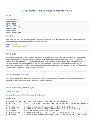
  • 11. Understandanding the relationship between various numerical parameter and audience score Graph the runtime predictor Checking the relationship between runtime (explanatory variable) and audience score (response variable) by plotting using the code below. ggplot(MD, aes(x=runtime, y=audience_score)) + geom_point() + stat_smooth(method=lm, level=0.99) Discussion The relationship is a positive weak liner relationship between a potential explanatory variable (predictor) and the response variable as depicted in the graph. This Relationship should be confirmed by the Corelation matrix (done below). Graph the rel_year predictor Checking the relationship between rel_year (explanatory variable) and audience score (response variable) by plotting using the code below. ggplot(MD, aes(x=rel_year, y=audience_score)) + geom_point() + stat_smooth(method=lm, level=0.99)
  • 12. Discussion There seems to be no relationship between a potential explanatory variable (predictor) and the response variable as depicted in the graph. This Relationship should be confirmed by the Corelation matrix (done below). Graph the rel_month predictor Checking the relationship between rel_month (explanatory variable) and audience score (response variable) by plotting using the code below. ggplot(MD, aes(x=rel_month, y=audience_score)) + geom_point() + stat_smooth(method=lm, level=0.99)
  • 13. Discussion There seems to be no relationship between a potential explanatory variable (predictor) and the response variable as depicted in the graph. This Relationship should be confirmed by the Corelation matrix (done below). Graph the imdb_rating predictor Checking the relationship between imdb_rating (explanatory variable) and audience score (response variable) by plotting using the code below. ggplot(MD, aes(x=imdb_rating, y=audience_score)) + geom_point() + stat_smooth(method=lm, level=0.99)
  • 14. Discussion There seems to be strong positive linear relationship between a potential explanatory variable (predictor) and the response variable as depicted in the graph. This Relationship should be confirmed by the Corelation matrix (done below). Graph the imdb_num_votes predictor Checking the relationship between imdb_num_votes (explanatory variable) and audience score (response variable) by plotting using the code below. ggplot(MD, aes(x=imdb_num_votes, y=audience_score)) + geom_point() + stat_smooth(method=lm, level=0.99)
  • 15. Discussion There seems to be a moderate positive linear relationship between a potential explanatory variable (predictor) and the response variable as depicted in the graph. This Relationship should be confirmed by the Corelation matrix (done below). Graph the critics_score predictor Checking the relationship between imdb_num_votes (explanatory variable) and audience score (response variable) by plotting using the code below. ggplot(MD, aes(x=critics_score, y=audience_score)) + geom_point() + stat_smooth(method=lm, level=0.99)
  • 16. Discussion There seems to be a strong positive linear relationship between a potential explanatory variable (predictor) and the response variable as depicted in the graph. This Relationship should be confirmed by the Corelation matrix (done below). Creating a Corelation Matrix and Graphing it Corelation matrix was created using the code below. # Selecting the numerical data MD[ , sapply(MD, is.numeric)] ## # A tibble: 650 x 7 ## runtime rel_year rel_month imdb_rating imdb_num_votes critics_score ## <dbl> <dbl> <dbl> <dbl> <int> <dbl> ## 1 80 2013 4 5.5 899 45 ## 2 101 2001 3 7.3 12285 96 ## 3 84 1996 8 7.6 22381 91 ## 4 139 1993 10 7.2 35096 80 ## 5 90 2004 9 5.1 2386 33 ## 6 78 2009 1 7.8 333 91 ## 7 142 1986 1 7.2 5016 57 ## 8 93 1996 11 5.5 2272 17 ## 9 88 2012 9 7.5 880 90 ## 10 119 2012 3 6.6 12496 83 ## # ... with 640 more rows, and 1 more variables: audience_score <dbl> # applying the numerical data to get correlation CorMatrix <- cor(MD[ ,sapply(MD,is.numeric)], use= "complete.obs") corrplot(CorMatrix, method="shade", shade.col=NA, cl.pos="n", tl.col="black", tl.srt=30, addCoef.col="black")
  • 17. Discussion The correlation matrix gives the following corelationship coefficient between the numeric predictor and reponse variable which is audience_score is as below. SNo. Predictor Correlation Coeff. Linear Relationship 1. runtime 0.18 +ve, weak relationship 2. rel_year -0.05 no relationship 3. rel_month 0.03 no relationship 4. imdb_rating 0.86 +ve, very strong 5. imdb_num_votes 0.29 +ve, moderate 6. critics_score 0.70 +ve, strong In the correlation matrix it can be seen that the collinearty between two explanatory variable imdb_rating and critics_score. the relationship between these two is exceptionally strong which is 76% and it means that the two variables contribute redundant information to the model and complicate model estimation. Hence the explanatory variable, critics_score will not be used. However the extremely high correlation between imdb_rating and audience_score of 86% indicates that imdb_rating should be the first predictor added to the model. Part 4: Modeling Developing the Model To create a Multiple Linear Regression (MLR) model that predicts audience score (AS), adding predictor with Forwad Stepwise Regression methodology has been selected. To build/create the multiple regression model a iterative process is used. the model will be build using the lm() function, Summarizing the model and to analyze its adjusted R square the summary function is used. To add the predictor to the model by analyzing both the AIC & p-value, add() function is used. This approach was used because it evaluated both the significance (as measured by both F-values and t-values) and the proportion of variability (as measured by adjusted R-square) before a predictor is added.
  • 18. Create blank Model for audience score Create a blank model for audience score (response variable) using the code below. # Multiple Linear Regression Model for Audience Score MLRMAS <- lm(audience_score~1, data=MD) Summarze the existing model ascertain significane, adjusted R-square, is increasing & the degree of freedom are decreasing summary(MLRMAS) ## ## Call: ## lm(formula = audience_score ~ 1, data = MD) ## ## Residuals: ## Min 1Q Median 3Q Max ## -51.348 -16.348 2.652 17.652 34.652 ## ## Coefficients: ## Estimate Std. Error t value Pr(>|t|) ## (Intercept) 62.3477 0.7937 78.56 <2e-16 *** ## --- ## Signif. codes: 0 '***' 0.001 '**' 0.01 '*' 0.05 '.' 0.1 ' ' 1 ## ## Residual standard error: 20.23 on 649 degrees of freedom Discussion Only the intercept is in the model and there is no predictor. However the degree of freedom is 649 (650-0-1). Selecting the first predictor To select the first predictor we need to find the predictor with the lowest AIC and p-value. The table to check the values can the displayed using the code below. add1(MLRMAS, scope=MD, test="F") ## Warning in model.matrix.default(Terms, m, contrasts.arg = object ## $contrasts): the response appeared on the right-hand side and was dropped ## Warning in model.matrix.default(Terms, m, contrasts.arg = object ## $contrasts): problem with term 11 in model.matrix: no columns are assigned ## Single term additions ## ## Model: ## audience_score ~ 1 ## Df Sum of Sq RSS AIC F value Pr(>F) ## <none> 265727 3910.6 ## genre 10 51633 214094 3790.2 15.4108 < 2.2e-16 *** ## runtime 1 8702 257025 3891.0 21.9389 3.431e-06 *** ## mpaa_rating 5 18017 247710 3875.0 9.3684 1.248e-08 *** ## rel_year 1 798 264930 3910.7 1.9516 0.1629 ## rel_month 1 273 265455 3911.9 0.6660 0.4147 ## imdb_rating 1 198782 66945 3016.5 1924.1205 < 2.2e-16 *** ## imdb_num_votes 1 22393 243335 3855.4 59.6321 4.353e-14 *** ## critics_score 1 131758 133970 3467.5 637.3000 < 2.2e-16 *** ## critics_rating 2 100258 165469 3606.7 196.0095 < 2.2e-16 *** ## audience_rating 1 198625 67102 3018.0 1918.1116 < 2.2e-16 *** ## audience_score 0 0 265727 3910.6
  • 19. ## --- ## Signif. codes: 0 '***' 0.001 '**' 0.01 '*' 0.05 '.' 0.1 ' ' 1 Discussion As expected, the significant predictor with the lowest AIC is imdb_rating (3016.5). significance is determined by using F-value which is very high consequently the p-value is less than 0.05. Adding the first predictor to model The selected predictor is added to the model using the code below. MLRMAS <- lm(audience_score~imdb_rating, data=MD) Summarizing the first iteration Ascertain Significance, adjusted R square is increasing and degree of freedom are decreasing. The model can the summarize using the code below. summary(MLRMAS) ## ## Call: ## lm(formula = audience_score ~ imdb_rating, data = MD) ## ## Residuals: ## Min 1Q Median 3Q Max ## -26.805 -6.550 0.676 5.676 52.912 ## ## Coefficients: ## Estimate Std. Error t value Pr(>|t|) ## (Intercept) -42.3748 2.4205 -17.51 <2e-16 *** ## imdb_rating 16.1321 0.3678 43.87 <2e-16 *** ## --- ## Signif. codes: 0 '***' 0.001 '**' 0.01 '*' 0.05 '.' 0.1 ' ' 1 ## ## Residual standard error: 10.16 on 648 degrees of freedom ## Multiple R-squared: 0.7481, Adjusted R-squared: 0.7477 ## F-statistic: 1924 on 1 and 648 DF, p-value: < 2.2e-16 Discussion After adding the imdb_rating predictor to the model, three were examined: 1. t-value to confirm a significant p-value 2. adjuste R square to confirm an increase 3. degrees of freedom to confirm a decrease. All three were confirmed. Note the values of Multiple R-squared: 0.748, Adjusted R-squared: 0.7477, DF: 648, p-value: <2.2e-16. Selecting the second predictor To select the second predictor we need to find the predictor with the lowest AIC and p-value. The table to check the values can the displayed using the code below. add1(MLRMAS, scope=MD, test="F") ## Warning in model.matrix.default(Terms, m, contrasts.arg = object ## $contrasts): the response appeared on the right-hand side and was dropped ## Warning in model.matrix.default(Terms, m, contrasts.arg = object ## $contrasts): problem with term 11 in model.matrix: no columns are assigned
  • 20. ## Single term additions ## ## Model: ## audience_score ~ imdb_rating ## Df Sum of Sq RSS AIC F value Pr(>F) ## <none> 66945 3016.5 ## genre 10 4589 62357 2990.4 4.6949 1.706e-06 *** ## runtime 1 746 66199 3011.2 7.2904 0.0071137 ** ## mpaa_rating 5 1016 65929 3016.6 1.9816 0.0794436 . ## rel_year 1 204 66742 3016.6 1.9753 0.1603687 ## rel_month 1 231 66714 3016.3 2.2414 0.1348464 ## imdb_num_votes 1 3 66943 3018.5 0.0260 0.8719136 ## critics_score 1 1167 65779 3007.1 11.4745 0.0007483 *** ## critics_rating 2 1976 64969 3001.1 9.8231 6.273e-05 *** ## audience_rating 1 35703 31242 2523.2 739.3758 < 2.2e-16 *** ## audience_score 0 0 66945 3016.5 ## --- ## Signif. codes: 0 '***' 0.001 '**' 0.01 '*' 0.05 '.' 0.1 ' ' 1 Discussion audience_rating is the next significant predictor with the lowest AIC (2523.2). Significance is determined by using F-value which is very high consequently the p-value is less than 0.05. Adding the second predictor to model The selected predictor is added to the model using the code below. MLRMAS <- lm(audience_score~imdb_rating + audience_rating, data=MD) Summarizing the second iteration Ascertain Significance, adjusted R square is increasing and degree of freedom are decreasing. The model can the summarize using the code below. summary(MLRMAS) ## ## Call: ## lm(formula = audience_score ~ imdb_rating + audience_rating, ## data = MD) ## ## Residuals: ## Min 1Q Median 3Q Max ## -22.1512 -4.7629 0.6289 4.3517 24.3283 ## ## Coefficients: ## Estimate Std. Error t value Pr(>|t|) ## (Intercept) -11.5316 2.0062 -5.748 1.39e-08 *** ## imdb_rating 9.5271 0.3496 27.251 < 2e-16 *** ## audience_ratingUpright 20.8584 0.7671 27.191 < 2e-16 *** ## --- ## Signif. codes: 0 '***' 0.001 '**' 0.01 '*' 0.05 '.' 0.1 ' ' 1 ## ## Residual standard error: 6.949 on 647 degrees of freedom ## Multiple R-squared: 0.8824, Adjusted R-squared: 0.8821 ## F-statistic: 2428 on 2 and 647 DF, p-value: < 2.2e-16 Discussion After adding the imdb_rating predictor to the model, three were examined: 1. t-value to confirm a significant p-value
  • 21. 2. adjuste R square to confirm an increase 3. degrees of freedom to confirm a decrease. All three were confirmed. Note the values of Multiple R-squared: 0.8824, Adjusted R-squared: 0.8821, DF: 647, p-value: <2.2e-16. Selecting the third predictor To select the second predictor we need to find the predictor with the lowest AIC and p-value. The table to check the values can the displayed using the code below. add1(MLRMAS, scope=MD, test="F") ## Warning in model.matrix.default(Terms, m, contrasts.arg = object ## $contrasts): the response appeared on the right-hand side and was dropped ## Warning in model.matrix.default(Terms, m, contrasts.arg = object ## $contrasts): problem with term 11 in model.matrix: no columns are assigned ## Single term additions ## ## Model: ## audience_score ~ imdb_rating + audience_rating ## Df Sum of Sq RSS AIC F value Pr(>F) ## <none> 31242 2523.2 ## genre 10 1265.01 29977 2516.3 2.6881 0.00313 ** ## runtime 1 240.18 31002 2520.2 5.0047 0.02562 * ## mpaa_rating 5 399.93 30842 2524.8 1.6650 0.14093 ## rel_year 1 67.08 31175 2523.8 1.3900 0.23884 ## rel_month 1 126.78 31116 2522.5 2.6321 0.10521 ## imdb_num_votes 1 8.67 31234 2525.0 0.1793 0.67210 ## critics_score 1 140.61 31102 2522.2 2.9205 0.08794 . ## critics_rating 2 154.79 31088 2523.9 1.6057 0.20154 ## audience_score 0 0.00 31242 2523.2 ## --- ## Signif. codes: 0 '***' 0.001 '**' 0.01 '*' 0.05 '.' 0.1 ' ' 1 Discussion genre is the next significant predictor with the lowest AIC (2516.3). Significance is determined by using F-value which is very high consequently the p-value is less than 0.05. Adding the third predictor to model The selected predictor is added to the model using the code below. MLRMAS <- lm(audience_score~imdb_rating + audience_rating + genre, data=MD) Summarizing the third iteration Ascertain Significance, adjusted R square is increasing and degree of freedom are decreasing. The model can the summarize using the code below. summary(MLRMAS) ## ## Call: ## lm(formula = audience_score ~ imdb_rating + audience_rating + ## genre, data = MD) ## ## Residuals: ## Min 1Q Median 3Q Max ## -21.6395 -4.4288 0.5889 4.2970 25.0845
  • 22. ## ## Coefficients: ## Estimate Std. Error t value Pr(>|t|) ## (Intercept) -12.5605 2.1955 -5.721 1.63e-08 *** ## imdb_rating 9.8028 0.3689 26.571 < 2e-16 *** ## audience_ratingUpright 20.3180 0.7746 26.231 < 2e-16 *** ## genreAnimation 3.6228 2.4513 1.478 0.13991 ## genreArt House & International -2.7912 2.0320 -1.374 0.17005 ## genreComedy 1.5109 1.1269 1.341 0.18050 ## genreDocumentary 0.6003 1.3696 0.438 0.66130 ## genreDrama -0.8339 0.9589 -0.870 0.38481 ## genreHorror -1.6199 1.6693 -0.970 0.33222 ## genreMusical & Performing Arts 2.5416 2.1899 1.161 0.24625 ## genreMystery & Suspense -3.2744 1.2462 -2.627 0.00881 ** ## genreOther 0.2743 1.9251 0.142 0.88675 ## genreScience Fiction & Fantasy 0.2559 2.4406 0.105 0.91652 ## --- ## Signif. codes: 0 '***' 0.001 '**' 0.01 '*' 0.05 '.' 0.1 ' ' 1 ## ## Residual standard error: 6.86 on 637 degrees of freedom ## Multiple R-squared: 0.8872, Adjusted R-squared: 0.8851 ## F-statistic: 417.5 on 12 and 637 DF, p-value: < 2.2e-16 Discussion After adding the imdb_rating predictor to the model, three were examined: 1. t-value to confirm a significant p-value 2. adjuste R square to confirm an increase 3. degrees of freedom to confirm a decrease. All three were confirmed. Note the values of Multiple R-squared: 0.8872, Adjusted R-squared: 0.8851, DF: 637, p-value: <2.2e-16. Selecting the fourth predictor To select the second predictor we need to find the predictor with the lowest AIC and p-value. The table to check the values can the displayed using the code below. add1(MLRMAS, scope=MD, test="F") ## Warning in model.matrix.default(Terms, m, contrasts.arg = object ## $contrasts): the response appeared on the right-hand side and was dropped ## Warning in model.matrix.default(Terms, m, contrasts.arg = object ## $contrasts): problem with term 11 in model.matrix: no columns are assigned ## Single term additions ## ## Model: ## audience_score ~ imdb_rating + audience_rating + genre ## Df Sum of Sq RSS AIC F value Pr(>F) ## <none> 29977 2516.3 ## runtime 1 107.425 29870 2516.0 2.2873 0.13093 ## mpaa_rating 5 114.492 29863 2523.8 0.4846 0.78787 ## rel_year 1 102.085 29875 2516.1 2.1732 0.14093 ## rel_month 1 169.321 29808 2514.6 3.6127 0.05779 . ## imdb_num_votes 1 21.772 29956 2517.8 0.4622 0.49682 ## critics_score 1 121.255 29856 2515.7 2.5830 0.10851 ## critics_rating 2 154.302 29823 2516.9 1.6427 0.19427 ## audience_score 0 0.000 29977 2516.3 ## --- ## Signif. codes: 0 '***' 0.001 '**' 0.01 '*' 0.05 '.' 0.1 ' ' 1
  • 23. Discussion There is no next significant predictor to add to the model with p-value less than 0.05. Analyze the final model Analyzing the the final model's regression output, avona output and the formula using the code written below. summary(MLRMAS) ## ## Call: ## lm(formula = audience_score ~ imdb_rating + audience_rating + ## genre, data = MD) ## ## Residuals: ## Min 1Q Median 3Q Max ## -21.6395 -4.4288 0.5889 4.2970 25.0845 ## ## Coefficients: ## Estimate Std. Error t value Pr(>|t|) ## (Intercept) -12.5605 2.1955 -5.721 1.63e-08 *** ## imdb_rating 9.8028 0.3689 26.571 < 2e-16 *** ## audience_ratingUpright 20.3180 0.7746 26.231 < 2e-16 *** ## genreAnimation 3.6228 2.4513 1.478 0.13991 ## genreArt House & International -2.7912 2.0320 -1.374 0.17005 ## genreComedy 1.5109 1.1269 1.341 0.18050 ## genreDocumentary 0.6003 1.3696 0.438 0.66130 ## genreDrama -0.8339 0.9589 -0.870 0.38481 ## genreHorror -1.6199 1.6693 -0.970 0.33222 ## genreMusical & Performing Arts 2.5416 2.1899 1.161 0.24625 ## genreMystery & Suspense -3.2744 1.2462 -2.627 0.00881 ** ## genreOther 0.2743 1.9251 0.142 0.88675 ## genreScience Fiction & Fantasy 0.2559 2.4406 0.105 0.91652 ## --- ## Signif. codes: 0 '***' 0.001 '**' 0.01 '*' 0.05 '.' 0.1 ' ' 1 ## ## Residual standard error: 6.86 on 637 degrees of freedom ## Multiple R-squared: 0.8872, Adjusted R-squared: 0.8851 ## F-statistic: 417.5 on 12 and 637 DF, p-value: < 2.2e-16 anova(MLRMAS) ## Analysis of Variance Table ## ## Response: audience_score ## Df Sum Sq Mean Sq F value Pr(>F) ## imdb_rating 1 198782 198782 4224.0003 < 2e-16 *** ## audience_rating 1 35703 35703 758.6665 < 2e-16 *** ## genre 10 1265 127 2.6881 0.00313 ** ## Residuals 637 29977 47 ## --- ## Signif. codes: 0 '***' 0.001 '**' 0.01 '*' 0.05 '.' 0.1 ' ' 1 formula(MLRMAS) ## audience_score ~ imdb_rating + audience_rating + genre Discussion The final model depicts a Parsimonius Model: the simplest model with the highest predictive power. Only three predictors are used : imdb_rating, audience_rating and genre.
  • 24. The ANOVA output confirms the significance of the individual predictors (i.e., p-values < 0.05) The linear regression model output confirm the significance of the individual predictors as well, but it also confirms the significance of the model as a whole (i.e., F-statistic 417.5 on 12 and 637 DF, p-value:< 2.2e-16). Finally, the proportion of variability in the response variable explained by the model is 88.51% (i.e. adjusted R- square). Variables that were excluded from the table are listed below- runtime - weak linear relationship and not significant rel_year - no linear relationship and not significant rel_month - no linear relationship and not significant mpaa_rating - not significant imdb_num_votes - not significant critics_rating - not significant critics_score - collinearity and not significant Intrepreting the coefficients To know of the coefficient of the model use the code below. coefficients(MLRMAS) ## (Intercept) imdb_rating ## -12.5605354 9.8028449 ## audience_ratingUpright genreAnimation ## 20.3180279 3.6228430 ## genreArt House & International genreComedy ## -2.7911586 1.5108717 ## genreDocumentary genreDrama ## 0.6003104 -0.8339436 ## genreHorror genreMusical & Performing Arts ## -1.6198585 2.5415754 ## genreMystery & Suspense genreOther ## -3.2743845 0.2742760 ## genreScience Fiction & Fantasy ## 0.2559299 Discussion the interpretation of a multivariate regression coefficient is the expected change in the response per unit change in a predictor, holding all of the other predictors constant. Specific interpretations follow- • Intercept Coefficient: the estimated audience score is -12.56053 if none of the predictors in the model are included. this cn be interpreted as that if no information is given the audience generally conceive the movie with a negative sense. • imdb_rating: the estimated expected increase in the audience score is 9.8028 when the imdb_rating goes up by 1, holding all other predictors constant. • audience_rating Upright coefficient: the estimted audience_rating score is 20.318, ehen the audience rating is "Upright " and holding all other predictors constant. However if the audience rating is "Spilled" the expected decrease in audience score will be of around 20. • genreDrama Coefficient: the estimated decrease in audience score, when the genre is drama is 0.83394, while holding all other predictor constant. However, the audience scores can increase or decrease depending on what genre category is selected.
  • 25. Model Diagnostics i.e. Checking the conditions graphically Check for linearity Checking for the linear relationship between numerical predictor (s) and residual (s) using the code written below. plot(MLRMAS$residuals ~ MD$imdb_rating, main="Linearity Condition") Discussion Condition met the plot depicts a complete random scatter around zero; no descernable pattern. Check for normality Checking for the nearly normal residuals using the code written below. qqnorm(MLRMAS$residuals, main="Normality Condition") qqline(MLRMAS$residuals, main="Normality Condition")
  • 26. Discussion Condition met - the majority of the points lie on the line, but because of skeness, a few points do not. Also note that there are no apparent outliners. hist(MLRMAS$residuals, prob=TRUE, main="Normality Condition") lines(density(MLRMAS$residuals), col="blue", lwd=2)
  • 27. Discussion Condition met - the histogram confirms the skewness (right skewness) but the distribution still appear to be nearly normal. Check for variability checking for the variability of the residuals using the code written below. plot(MLRMAS$residuals ~ MLRMAS$fitted.values, main="Variability conditions") Discussion Condition met - the plot of predicted values shows that residuals are equally variable for low and heigh values and there is no visible fan pattern. plot(abs(MLRMAS$residuals) ~ MLRMAS$fitted.values, main="Variability conditions")
  • 28. Discussion Condition met - the plot of absolute value of the residuals does not depict any unusual observations. Check for independancy checking for the independancy of the residuals using the code written below. plot(MLRMAS$residuals, main="Independany Conditions")
  • 29. Discussion Condition met - the plot depicts residuals being randomly scatterd around zero. Part 5: Prediction Building a test data case Build test data cases for the movie "Deadpool (2016)" using the data gathered from IMDB and rotten tomatoes website and storing the data in the variable named TDC (test data case) using the following code. audience_score <- 90 imdb_rating <- 8.1 audience_rating <- "Upright" genre <- "Comedy" TDC <- data.frame (audience_score, imdb_rating, audience_rating, genre) Discussion: as said above the source of the data is IMDB and rotten tomatatoes website. once the movie was selected the movie ws searched on these two website and the reuired data was extracted which will be used here. Predicting the audience score TDC (test data case) using the following code. myPrediction <- round(predict(MLRMAS, TDC), digits = 0) c(myPrediction, TDC$audience_score) ## 1 ## 89 90 Discussion: Predicting the correct audience score was not easy. The model seems to be much sensitive to the imdb_rating variable and the result of this sesitivity was to predict a much higher audience score. Audience score will be predicted much more accurately by the model when both the audience acore and the imdb_rating are relatively high. Estimate and Interpret the prediction confidence interval ConfidenceInterval <- predict(MLRMAS, TDC, interval="confidence") ConfidenceInterval ## fit lwr upr ## 1 88.67141 86.72074 90.62207 Discussion: We are 95% confident that, all else being equal, the predicted audience score for the movie 'Deadpool' will be between 86.72074 and 90.62207 on average. Part 6: Conclusion Explanatory data analysis was of great help in providing the insight on what data items to include in the model or not to. The modeling methodology of evaluating both significance and variablity of each predictor before adding it to the
  • 30. model produced a very robust model that very precisely answered the research question and the model predicted the audience score correctly and the margin of error is +/- (90.62207-86.72074) =1.950665. State Concerns Sample is not representative: the data is biased toward drama movies, consequently the model was trained primarily by drame movie dataset thus it would have been better to predict the audience score about drama movies.