Social origins of inventors

The Social Origins of Inventors∗
Philippe Aghion Ufuk Akcigit Ari Hyytinen Otto Toivanen
November 29, 2017
Abstract
In this paper we merge three datasets - individual income data, patenting data,
and IQ data - to analyze the deterninants of an individual’s probability of inventing.
We find that: (i) parental income matters even after controlling for other background
variables and for IQ, yet the estimated impact of parental income is greatly dimin-
ished once parental education and the individual’s IQ are controlled for; (ii) IQ has
both a direct effect on the probability of inventing an indirect impact through edu-
cation. The effect of IQ is larger for inventors than for medical doctors or lawyers.
The impact of IQ is robust to controlling for unobserved family characteristics by
focusing on potential inventors with brothers close in age. We also provide evi-
dence on the importance of social family interactions, by looking at biological versus
non-biological parents. Finally, we find a positive and significant interaction effect
between IQ and father income, which suggests a misallocation of talents to innova-
tion.
Keywords: Inventors, innovation, social mobility, IQ, education, parental back-
ground.
JEL Classifications: O31, I24, J18.
∗Addresses- Aghion: College de France and London School of Economics (P.Aghion@lse.ac.uk).
Akcigit: University of Chicago (uakcigit@uchicago.edu). Hyytinen: University of Jyvaskyla
(ari.t.hyytinen@jyu.fi). Toivanen: Aalto University School of Business and KU Leuven
(otto.toivanen@aalto.fi). This project owes a lot to early discussions with Raj Chetty, Xavier Jaravel
and John Van Reenen when we were embarking on two parallel projects, them on US inventors and us
on Finnish inventors. We also benefitted from very helpful comments and suggestions from our discus-
sants at the NBER Summer Institute and at the AEA meetings, namely Pierre Azoulay, Chad Jones, and
Heidi Williams respectively, and also from seminar participants at the University of Chicago, the Kaufman
Foundation, the Paris School of Economics, the London School of Economics, the IOG group at the Cana-
dian Institute for Advanced Research, the Institute of Fiscal Studies, HECER, the University of Maastricht,
Copenhagen Business School, EIEF and College de France.

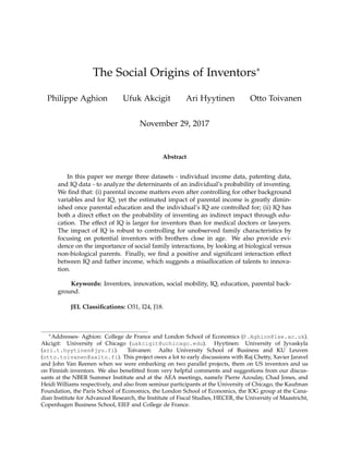
The Social Origins of Inventors
1 Introduction
Who becomes an inventor? Does innovation attract the most talented individuals or is
there misallocation of talents into innovation? In practice, not everybody can become an
innovator: whether one becomes an innovator or not is likely to depend upon the social
environment (e.g., parental resources and education) and upon ability. To the extent
that both parental inputs and ability are unevenly distributed across individuals, the
innovative potential of the economy may be underutilized due to misallocation of talent.
Misallocation means that a positive fraction of potential inventors are not performing
as well as they could due to inadequate or insufﬁcient parental support. Inadequate
parental support may be especially harmful for highly talented individuals, eroding
even further the utilization of the innovative potential of the economy.
In this paper we merge three comprehensive Finnish datasets to analyze the determi-
nants of an individual’s probability to become an inventor, and to investigate whether
and to which extent there is a misallocation of talents to innovation.1 We thus consider
in detail the role of: (i) family resources, parental education and social background;
(ii) innate ability as proxied by visuospatial IQ; (iii) the interaction between parental
background and ability.
The following striking fact motivates our analysis. Figure 1 depicts the relationship
between an individual’s probability of becoming an inventor and his father’s income,
respectively on the basis of recent US data (Figure 1A is drawn from Bell et al., 2016),
on the basis of US historical data (Figure 1B is drawn from Akcigit et al., 2017), and
for Finland (Figure 1C is based on our own data). We see that in all three cases the
individual’s probability of becoming an inventor increases with father’s income, and that
the effect is highly non-linear, being particularly steep at the highest levels of father’s
income. We also see that the probability of innovating for an individual whose father is at
the very top of the income distribution is about ten times larger than the corresponding
probability for an individual with a father at the bottom end of the income distribution.
The similarity between Finland and the US is all the more remarkable given that, unlike
the US, Finland displays low income inequality and high social mobility in international
comparison (see Figure 2) and offers free education up to and including university. What
lies behind the steep relationship in Figure 1C between father income and the probability
of becoming an inventor in Finland?
To explore this enigma, we merge three Finnish data sets: (i) individual data on in-
come, education and other characteristics from Statistics Finland for individuals born
1In a companion paper (see Aghion et al., 2017), we analyze the return to innovation.
1

Figure 1: Parental Income and Becoming an Inventor
A. Source: Bell et al. (2016)
0.511.522.5
InventorsperTenThousand
0 20 40 60 80 100
Parent Income Percentile
B. Source: Akcigit et al. (2017)
0.01.02.03.04
Prob(inventor)
0 20 40 60 80 100
biol father's income percentile
C. Source: This paper.
Notes: The figure displays the probability to invent as a function of father’s / parents’ income percentile.
Figure 1A comes from Bell et al. (2016) and Figure 1 B from Akcigit etl al. (2017). In Figure 1C, father’s
income is measured in 1975 for individuals born 1961–1975, and in 1985 for individuals born in 1976-1985.
We calculate the percentile ranks using residuals from a regression of the natural log of deflated income
of fathers and mothers on year-of-birth dummies.
between 1961 and 1984, and their parents; (ii) individual patenting data from the Euro-
pean Patent Office; (iii) IQ data from the Finnish Defence Forces. Given that conscription
only affects males in Finland, we concentrate on the male workforce in this paper. We
analyze how family resources, social and educational background, own ability, and the
interaction between background and ability impact on an individual’s probability of
inventing.
2

Figure 2: The Great Gatsby Curve
Norway
Denmark
Finland
Canada
Australia
Sweden New Zealand
Germany
Japan
France
United States
Italy United Kingdom
0.1
0.15
0.2
0.25
0.3
0.35
0.4
0.45
0.5
0.55
19.5 21.5 23.5 25.5 27.5 29.5 31.5 33.5 35.5
SocialMobility(lessmobility→)
Inequality (more inequality →)
Source: Corak (2004)
Our main findings can be summarized as follows. First, parental income matters
for the probability of becoming an inventor, and it does so even after controlling for
other background variables and for IQ. Second, the estimated impact of parental income
is greatly diminished once parental socioeconomic status and education, and the indi-
vidual’s IQ are controlled for, dropping by 2/3rds. Third, IQ has both a direct effect
on the probability of inventing which is almost five times as large as that of having a
high-income father, and an indirect effect through education. Finally, the impact of IQ is
larger and more convex for inventors than for medical doctors or lawyers.
To address the potential endogeneity of IQ, we zoom our analysis on potential inven-
tors with brothers close in age. This allows us to control for family-specific time-invariant
unobservables. The effect of visuospatial IQ on the probability of inventing is robust to
adding these controls.
Next, we provide evidence on the importance of family structure by comparing indi-
viduals brought up by their biological parents with individuals with a missing biological
parent and/or individuals with a step parent. We find that parental divorce decreases
the probability of becoming an inventor and that the income of biological parents mat-
ters only when the child lives with them, but that the effect of parental education is not
dependent on living together.
We then explore the potential complementarity between IQ and family background.
We find a positive and significant interaction between the individual’s IQ and his father’s
3

income, which in turn points to a potential source of misallocation: namely, a positive
fraction of individuals with very high IQ will underperform as potential innovators due
to inadequate parental background.
The paper relates to several strands of literature. There is first a theoretical and
empirical literature on innovation incentives.2 However this literature does not look at
the effects of social background on the probability of inventing, nor do they analyze the
social mobility of inventors and co-workers.
Second, there is a recent literature on misallocation and economic growth. In partic-
ular Hsieh et al. (2013) look at how much of the increase in aggregate GDP per capita
between 1960 and 2010 is due to an improved allocation of talents to tasks in the US,
and in particular to an improved access of talented women or black men to high occu-
pation tasks. A key assumption in their analysis is that the distribution of innate ability
is identical across groups, and they point to the importance of labor market discrimina-
tion and of financial barriers to human capital investments as being key drivers of the
misallocation of talents in the US. Here, we do not make any prior assumption on the
distribution of ability across socioeconomic groups, and we focus on a country - Finland
- with a priori no or little labor market discrimination and where schooling is entirely
free. Yet, we find a significant misallocation of talent even in Finland, affecting high IQ
individuals in particular.
Third, our paper relates to the literature on innovation and social mobility. Thus
Frydman and Papanikolaou (2015) find that innovation and executive pay are positively
correlated at the firm level, but that pay inequality across executives and between exec-
utives and workers increases with innovation.3 Similarly, Balkin et al. (2000) finds that
innovation increases CEO pay in high-tech industries. Aghion et al. (2017) use the same
data that we use in the current paper to show that innovation increases an individual
innovator’s probability to make it to the higher income brackets, and that innovation
has an even larger effect on firm owners’ income. Bell et al. (2016) find that the most
successful innovators see a sharp rise in income. Akcigit et al. (2017) merge historical
census and patenting data across US states over the past 150 years and find a positive
correlation between patenting intensity and social mobility. Finally, building on Chetty
et al. (2014), Aghion et al. (2015) look at the relationship between innovation, inequality
and social mobility using aggregate cross-state and cross-commuting-zone data. They
2In particular, see Holmstrom (1989), Aghion and Tirole (1994), Pakes and Nitzan (1983), Scotchmer
(2004), Giuri et al. (2007), Franco and Mitchell (2008), Azoulay et al. (2010), Manso (2011), Akcigit et al.
(2016), and Depalo and Di Addario (2015).
3On CEO pay see also Gabaix and Landier (2008).
4

show that innovation measured by the flow or quality of patents is positively correlated
with the top 1% income share of income, is uncorrelated with broader measures of in-
come inequality, and is positively correlated with social mobility (measured as in Chetty
et al., 2014). In this paper our focus is on the relationship between parental education
and income, IQ and the individual’s probability of inventing.4
Closer to our analysis in this paper is a recent literature merging individual income
data with individual patenting data. First, Toivanen and Väänänen (2012) use Finnish
patent and income data to study the return to inventors of US patents. They find strong
and long-lasting impacts, especially for the inventors of highly cited patents. Toivanen
and Väänänen (2016) look at the effect of education on the probability of becoming an
inventor and they find a positive and significant treatment effect, suggesting the one may
increase innovation through education policy. Second, Celik (2015) matches inventors’
surnames with socioeconomic background information inferred from those surnames by
looking at the US census data back in 1930. His main finding is that individuals from
richer backgrounds are far more likely to become inventors. Akcigit et al. (2017) merge
historical patent and individual census records and show that probability of becoming an
inventor around 1940s was very highly correlated with father’s income but this strong
relationship disappears once child’s education is controlled for. Finally, Jaravel et al.
(2015) merge US individual tax data and individual patenting data to quantify the impact
of coauthors in the career of inventors, finding evidence of large spillover effects.5
Most closely related to the present paper, is Bell et al. (2016) who merge US indi-
vidual fiscal and test score data with US patenting data over a recent period to look at
the lifecycle of inventors and the returns to invention. These authors find that parental
income, parental occupation and sector of activity, race, gender, and childhood neigh-
borhood are important determinants of the probability of becoming an inventor. Our
analysis complements theirs, as on the one hand, we do not have as detailed informa-
tion as they do on parents’ inventive activity or on geographical origins, but on the other
hand we have information on parental socioeconomic status and education, individual
IQ, and family structure.
4Our paper intersects with the psychology literature and the debate on whether IQ tests are linked to
genetics or to the social environment (e.g. see Mc Gue et al., 1993; Ceci, 2001; Pinker, 2005; and Plomin
and Spinath, 2004). And our emphasis on (visuospatial) IQ as a measure of cognitive ability is shared by
recent work by Dal Bó et al. (2017) who use similar IQ test information from the Swedish Arm Forces to
analyze the selection of municipal politicians in Sweden.
5Jaravel’s work builds on prior seminal work by Azoulay et al. (2010) which examines the effect of the
premature death of 112 eminent scientists on their co-authors. This work provides the first convincing
evidence of exposure to human capital (particularly at the high end) on the production of new scientific
ideas, using the exogenous passing of elite scientists as an empirical lever.
5

The information on parental socioeconomic status and education allows us to show
that to a large extent in Finland the relationship between parental income and the proba-
bility of becoming an inventor is driven by parental education both directly and through
its impact on the child’s education. The information on IQ allows us to show that IQ
impacts both directly and indirectly through education on the probability of becoming
an inventor, and that it is more important than parental characteristics. Finally, the infor-
mation on family structure allows us to identify how the effects of income and education
of biological parents on the probability of inventing is affected by (not) living with them,
and what effect the income of genetically unrelated step parents has on the probability
of becoming an inventor.
The remainder of the paper is organized as follows. Section 2 presents the data and
shows some descriptive statistics. Section 3 analyzes the determinants of becoming an
inventor. Section 4 focuses on potential innovators with close brothers to address the
concern that IQ is endogenous. Section 5 looks at the effect of family structure. Section
6 looks at the interaction between IQ and family background. Section 7 analyzes the
role of education in becoming an inventor. Finally, Section 8 concludes by drawing some
policy conclusions and by suggesting avenues for future research. Appendix A contains
additional tables. Appendices B–G, which are online, present various supplementary
materials.
2 Data and descriptive statistics
2.1 Data sources
Our data come from the following sources.
First data source: Statistics Finland (SF). We exploit two data sets from SF: (i) The
Finnish Linked Employer-Employee Data (FLEED) for the period 1988-2012 and (ii) the
population census 1975 and 1985.
FLEED covers the whole working age (15 and older) population of Finland. This
annual panel is constructed from administrative registers of individuals, firms and es-
tablishments, maintained by SF. It includes information on individuals’ labor market
status, salaries and other sources of income extracted from tax and other administrative
registers. It also includes information on other individual characteristics. We utilize
information on individual age, location of residence, language, education (degree and
field) and socioeconomic status. We use FLEED data from 1988, the first year it is avail-
able, to 2013, the year our patent data ends. Because only a small minority of inventors
6

are women and because we only have IQ data for men, we exclude women from our
sample.
Information on parent characteristics is drawn from the population census. More
specifically, we use the population censuses of 1975 and 1985 for information about
parental education, socioeconomic status and income of biological and social parents.
The majority of individuals in our data have fathers born either in the 1940s (36%) or
1950s (25%). 37% of the individuals have mothers born in the 1940s and 30% mothers
born in the 1950s. For 45% of these individuals, the father has only a base education
(max. 9 years), while 6% have a Master’s degree or higher. The respective figures for
their mothers are 44% and 4%.
Second data source: the European Patent Office (EPO). EPO data provide information
on characteristics such as the inventor names and applicant names.6 We have collected
information on all patent applications to EPO with at least one inventor who registers
Finland as his or her place of residence. The data cover all EPO patent applications
(starting in 1978) with an inventor with a Finnish address up to and including 2013.
The data originates with PATSTAT, but Statistics Finland has used the OECD REGPAT
database built on PATSTAT. In the raw patent data, we have a total of 25,711 patent
applications and 17,566 inventors. The mean and median number of inventors per patent
is 2; the largest number of inventors per patent is 14.7 For each patent, we observe all the
inventors, their name and address, the patentee and its address, the number of citations
in the first 5 years, and the size of the patent family (i.e., the number of countries in
which the patent exists).
Third data source: the Finnish Defence Forces. The Finnish Defense Forces (FDF) pro-
vided us with information on IQ test results for conscripts who did their military service
in 1982 or later. These data contains the raw test scores of visuospatial, verbal and quan-
titative IQ tests. The IQ tests are a 2-hour multiple choice tests containing sections for
verbal, arithmetic and visuospatial reasoning. The latter is similar to the widely used
Raven’s Progressive Matrices – test. Overall, the Finnish Defense Force IQ test is similar
to the commonly used IQ tests; moreover, a large majority (over 75%) of each male co-
hort performs the military service and therefore takes the test: most conscripts take their
military service around the age of 20. All conscripts take the IQ test in the early stages
6 Here we want to thank the research project "Radical and Incremental Innovation in Industrial Re-
newal" by the VTT Research Centre (Hannes Toivanen, Olof Ejermo and Olavi Lehtoranta) for granting us
access to the patent-inventor data they compiled.
7As is typical, the distribution of the number of patents, and citations per patent (we use the number
of citations to the highest cited patent of an individual, measured over the first five years of the patent’s
life), are highly skewed - see Figure B1 and B2 in the Appendix.
7

of the service (see Jokela et al., 2017, for more detail).
We use the deciles in visuospatial IQ score (IQ henceforth for brevity), as it is consid-
ered in the IQ literature to be more strongly predetermined than the other two measures.
As is standard for IQ data, we normalize the raw test scores to have mean 100 and stan-
dard deviation of 15. We do this by the year of entering military service to avoid the
so-called Flynn effect. In robustness tests we use also the verbal and analytic IQ scores.8
Data matching: The linking of all other data but the patent data was done using
individual identifiers. The linking of patent data to individuals was done using the in-
formation on individual name (first and surname), employer name, individual address
and/or employer’s address (postcode, street name street number) and year of applica-
tion. These were used in different combinations, also varying the year of the match to be
before or after the year of application (e.g., matching a patent applied for in 1999 with
the street address of the firm from the registry taken in 1998 or 2000). The match rate
lies above 90%. We provide further details on data matching in Appendix B.1.
Sample: Our estimation sample contains all individuals for whom we were able
to match all four data sets (EPO, FLEED, parental data, IQ). This means that besides
women we exclude men born before 1961, as IQ data are not available for them. We
further exclude individuals born after 1984 as they are unlikely to have invented by
2012. The resulting cross-sectional sample comprises of around 350,000 individuals and
contains 4,754 inventors.
2.2 The institutional environment
In this section, we highlight some central features related to Finnish institutional envi-
ronment. A more detailed discussion is provided in Appendix B.2.
Overall economic environment in 1988-2012. During our observation period from
1988 to 2012, Finland’s gross domestic product (GDP) grew on average 2.1% per year.
Research and development (R&D) is a major investment item in Finland. R&D expendi-
tures reached their peak in 2011 when the total R&D expenditure by business sector and
public sector amounted to 3.8% of the GDP. Based on its Global Competitiveness Index,
World Economic Forum has quite consistently ranked Finland to be one of the ten most
8 Using similar IQ test information from the Swedish Arm Forces to analyze the selection of munic-
ipal politicians in Sweden, Dal Bó et al. (2017) argue that these IQ scores are good measures of general
intelligence and cognitive ability. The question remains as to whether IQ tests are linked to genetics or
to the social environment. The results of Pekkarinen et al. (2009) suggest that the Finnish comprehensive
school reform had no effect on visuospatial IQ, a marginally significant effect on analytic IQ, and a positive
impact on verbal IQ.
8

competitive countries in the world.
Educational system. A key characteristic of the Finnish education system is that
it is (essentially) free of charge at all levels, up to and including university studies (to
a PhD). Applicants to most field-specific degree programs of the Finnish polytechnics
and universities are required to take an entrance examination. Entry into degree pro-
grams in law and medicine, as well certain fields of science, technology and business, is
competitive.
Wage setting. Wage setting is a mixture of collective and individual mechanisms
in Finland. As Uusitalo and Vartiainen (2009) stress, for most employees in the man-
ufacturing sector the minimum wages rarely bind. These features of the Finnish labor
market mean that relative wages have largely been set by market forces and that wage
bargaining is to a significant extent local. Moreover, various firm-specific arrangements
and performance-related pay components became more widespread in the 1990s.
Remuneration of inventors. A specific law governs innovations made by employees
("Act on the Right in Employee Inventions", originally given in 1967, augmented in
2000). The provisions of the act apply to inventions (potentially) patentable in Finland.
In sum, the act assigns the right to ownership of an employee invention, but it does not
directly determine the amount firms have to pay if they exercise the right. Rather, the
determination of the amount of compensation is largely left to the market forces.
Economic inequality. In an international comparison, income inequality is rela-
tively low in Finland. Using disposable cash income (excl. capital gains) as the income
measure, the Gini-coefficient has ranged from 20.5 in 1992 to 26.4 in 2007 ( Income dis-
tribution statistics, Statistics Finland). On average, it has been 23.6 during our sample
period. Consistent with the relatively low income inequality, intergenerational mobility
is in Finland - like in other Nordic countries - quite high, exceeding that of the UK and
US (see, e.g., Black and Devereux, 2011). In line with this, the correlation of incomes
among siblings is quite a bit lower in Finland (and in the other Nordic countries) than,
for example, in the U.S. (Björklund et al., 2002, Black and Devereux, 2011).
2.3 Descriptive statistics on inventors and social origins
The outcome variables are (see Appendix B, Table B1 for precise variable definitions):
indicator variables first, for obtaining at least one patent (Inventor), being a medical
doctor (MD), being a lawyer (Lawyer), number of patents obtained by the individual
(Patent count), the number of forward citations obtained by the most cited patent of the
individual (Citations), and an indicator for having invented a highly cited patent (High
9

quality inventor).
The control variables we use are: age, region of residence (21 dummies), type of re-
gion (urban being the base, and indicator variables for semi-urban and rural), mother
tongue (Finnish, Swedish and any other language) and for parental birth-of-decade (sep-
arate vectors of indicator variables for father and mother). Our variables (vectors) of in-
terest are measures of parental wage, parental socioeconomic status, parental education,
and the individual’s own IQ.
We capture parental income by indicator variables for income quintiles, with separate
indicators for fathers and mothers. To allow for non-linearitiese at the right tail of the
income distribution, the highest income quintiles are divided into separate indicators for
the 81st – 90th percentiles, the 91st – 95th percentiles, and the 96th – 100th percentiles.
We use the 1975 (deﬂated) income from the census for parents of individuals born by
1975, and the 1985 census income information for parents of individuals born later than
1975. Income percentiles are based on the residuals of a log (wage) regression on year of
birth dummies.9
We divide parents into four socioeconomic groups: blue-collar, junior and senior
white-collar status, and others. We measure parental education by indicators for differ-
ent education levels. The levels are: base (= 9 years of schooling), secondary, college,
master’s degree and PhD. We also include indicators for a STEM education, separately
for both parents.
We include IQ using decile dummies. Just like with parental income, the highest
IQ decile is divided into separate indicators for the 91st – 95th and the 96th – 100th
percentiles.
Inventors are on average slightly older than the overall population in our sample (44
vs 41) and are: 1) more likely to have a father (but not a mother) in the 5 percent of the
income distribution (19 vs 8 percent); 2) less likely to have a blue-collar parent (29 vs
45 percent for fathers and 19 vs 31 for mothers) and more likely to have a white-collar
father; 3) more likely to have highly educated parents (19 (9) percent probability of father
(mother) having at least an MSc vs 6 (3) per cent) and more likely to have a mother (but
not father) with a STEM education (14 vs 5 percent); and 4) are more likely to be in the
top 5 per cent of the IQ distribution (19 vs 5 percent). All these differences are signiﬁcant
at the 1 percent level or better. We display the descriptive statistics in Appendix B, Table
B2, conditioning on the inventor status of the individual.
Figure 3 reproduces Figure 1 for Finnish data, adding the relationship between
9As a robustness test, we use an alternative income measure with no over-time variation.
10

mother’s income percentile and the probability to invent. We observe that fixing the
income percentile, the effect of mother’s income is larger than that of father’s. Further,
starting from roughly the 60th percentile, the effect of mother’s income starts to increase
faster than that of father’s income.10
Figure 3: Mother and Father’s Income and Becoming an Inventor
0.01.02.03.04.05
Prob(inventor)
0 20 40 60 80 100
biol parents' income percentile
father mother
Notes: The figure displays the probability to invent as a function of father’s and mother’s income per-
centile. Parental income is measured in 1975 for individuals born 1961–1975, and in 1985 for individuals
born in 1976–1985. We calculate the percentile ranks using residuals from a regression of the natural log
of deflated income of fathers and mothers on year-of-birth dummies.
Figure 4 displays histograms where the probability to invent is conditioned on parental
socioeconomic status, separately for fathers and mothers. The figure shows that those
with senior white-collar parents are about three times as likely to invent as those with
blue-collar parents. Parents are strongly positively assortatively matched along their
socio-economic status (see Figure B5 in the Appendix), and income and socioeconomic
status are positively correlated (Figure B6 in the Appendix). As an example, the aver-
10Notice that the distributions of mothers and fathers across the income percentiles are different, with a
higher fraction of mothers in the low end of the income distribution; see Figure B3 in the Appendix. We
observe positive assortative matching of parents regarding income. We display this association in Figure
B4.
11

age income percentile of blue-collar fathers is slightly above 60, but that of senior white
collar fathers about 90. The association is weaker for mothers.
Figure 4: Parental Socioeconomic Status and Becoming an Inventor
0.01.02.03
Prob(inventor)
0 1 2 3
NOTE: 0 = other 1 = bluec. 2 = jr whitec. 3 = sr whitec.
A. Father
0.01.02.03
Prob(inventor)
0 1 2 3
NOTE: 0 = other 1 = bluec. 2 = jr whitec. 3 = sr whitec.
B. Mother
Notes: The ﬁgure displays the probability to invent conditional on the socio-economic status of the father
(A) and mother (B). We divide parents into four groups by socioeconomic status: blue-collar, junior white
collar, senior white collar, and others. Parental socioeconomic status is measured in 1975 for parents born
before 1951, and in 1985 parents born in 1951 or thereafter.
Figure 5 displays histograms where the probability to invent is conditioned on parental
education, separately for fathers and mothers and for STEM and non-STEM education.
The ﬁgure shows clearly how the probability to invent is positively associated with the
level of both parents’ education, and conditional on the level of education, with the par-
ent having a STEM education. Those with a father or mother with a STEM PhD are more
than six times as likely to invent as those whose father or mother has only a base edu-
cation. Having a father or a mother with a STEM instead of a non-STEM PhD increases
the probability to invent by more than 50 percent.
Just like parental income and socio-economic status, parental education exhibits pos-
itive assortative matching. The probability that an individual whose father has a base
education has a mother also with base education is over 60 percent; if the father has a
PhD, the probability of the mother having at least an MSc is about 40 percent (Figure B7
in the Appendix). Education and income (Figure B8) and education and socioeconomic
status (Figure B9) of parents are positively correlated. As an example, the mean in-
come percentile of fathers with a base education is round 60, whereas the corresponding
number for fathers with a PhD is 90. The strong positive correlations of these parental
12

Figure 5: Parental Education Status and Becoming an Inventor
0.02.04.06.08
Prob(inventor)
1 2 3 4 5
NOTE: 1 = base educ. 2 = secondary 3 = college 4 = master 5 = PhD
non-science science
A. Father
0.02.04.06.08
Prob(inventor)
1 2 3 4 5
non-science science
B. Mother
Notes: The figure displays the probability to invent conditional on the education of the father (A) and
mother (B). We divide parents into five groups by level of education: base education (up to 9 years,
depending on age of parent), secondary, tertiary, MSc, and PhD. We also condition all other levels of
education but base education on a parent having a STEM education. A STEM base education does not
exist. Parental education is measured in 1975 unless unavailable, in which case 1985 data used.
characteristics suggest that one should control for all of them in exploring the relation
between parental background, income in particular, and the probability of becoming an
inventor.
We then turn to the association between own ability and inventing. Figure 6 plots the
probability to invent against IQ percentiles to allow for a comparison to Figures 1 and 3.
The probability to invent has an increasing and convex association with IQ. Comparing
individuals at the extreme right tail of the IQ distribution to those in the middle shows
that the former are five to six times more likely to invent than the latter.
Own IQ and parental income, socioeconomic status and education are all positively
correlated. We display the correlation between father’s and mother’s income and IQ
in Figure B10 in the Appendix. Both curves display an increasing, convex relationship.
Individuals whose parents are white collar have above average IQ (Figure B11 , as do
individuals with more educated parents (Figure B12).
Summarizing the descriptive statistics, Figures 3 - 6 suggest that parental income,
socioeconomic status and education as well as own IQ all are strongly positively associ-
ated with the probability to invent. In particular, the probability is highly convex at the
right end of the distribution for all parental characteristics and own IQ. These patterns
13

Figure 6: Own Visuo-Spatial IQ and Becoming an Inventor
0.02.04.06
Prob(inventor)
0 20 40 60 80 100
v-s IQ percentile
Notes: The ﬁgure displays the probability to invent conditional on the visuo-spatial IQ percentile of the
individual. IQ percentiles are calculated on the basis of the normalized IQ score, where normalization
was done separately for each conscription cohort to avoid the Flynn effect.
suggest potential misallocation of innovative talent.
3 Becoming an inventor
In this section, we study the determinants of becoming an inventor. In particular, we
estimate a linear probability model where we regress the probability of becoming an
inventor on base controls (see below), parental income, parental socioeconomic status,
parental education, and own IQ.
3.1 Regression equation
The regression equation that will serve as the basis for the estimations in this section can
be written as:
14

Di = α + ∑
f
βf f controlsf i + ∑
m
βmmcontrolsmi + ∑
k
θk IQki + ∑
o
βoocontrolsoi + i,
where: (i) D is a dummy for being an inventor / MD / lawyer (and in robustness tests,
patent count, count of citations to the most cited patent of the individual, and a dummy
for being a star inventor); (ii) the f controls variables measure father characteristics; (iii)
the mcontrols variables measure mother characteristics; (iv) the ocontrols variables mea-
sure other background characteristics; (v) the IQ variables measure the individual’s own
IQ; (vi) α, βs and θs are the parameters to be estimated; and (vii) is the error term.
Parental income is introduced via quintile indicators, with the highest quintile split
as explained above (fa income, mo income). The excluded income group for both parents
is the lowest quintile. The socioeconomic groups for both parents include "blue collar",
"white collar junior", and "white collar senior" (fa sose, mo sose, sose =bluecollar, jr
whitecollar, sr whitecollar). We take the "other" category as the base. For parental
education the excluded group is base education, and we use indicators for secondary,
college, masters, and PhD level education (fa educ, mo educ, educ =secondary, college,
MSc, PhD). We also include separate dummies to indicate that a parent has a STEM
education (fa STEM, mo STEM). For IQ, the base group is the 4th IQ decile; and we
include dummies for 1st - 3rd and 5th - 9th IQ deciles (IQd); we split the highest decile
into two separate dummies for 91st-95th and 96th-100th percentiles. Finally, we include
in all specifications the following control variables: a 4th order polynomial in (log) age,
21 region dummies; dummies for suburban and urban areas; dummies for Swedish and
other than Finnish language as mother tongue; and parental decade of birth dummies,
separately for both parents.
3.2 Baseline results
The regression results are shown in Table 1. Since these are very lengthy regressions
with too many independent variables, we report here only the coefficients of the most
interesting variables.11
In column 1 of Table 1 we regress D on base controls and parental income. We
see from column 1 in Table 1 that having either the father or the mother belong to the
second highest 91-95 or the highest 96-100 income bracket has a positive and significant
association with the probability of becoming an inventor. Comparing the coefficients of
the order of more than 1 and 2 percentage points to the sample mean of 0.9 percent for
11Tables displaying the coefficients of all but control variables can be found in Appendix Table C1.
15

Table 1: Who Becomes Inventor Regressions
VARIABLES (1) (2) (3) (4)
fa income 91-95 0.0149*** 0.00919*** 0.00684*** 0.00515***
(0.00107) (0.00109) (0.00109) (0.00108)
fa income 96-100 0.0246*** 0.0154*** 0.00938*** 0.00745***
(0.00126) (0.00131) (0.00130) (0.00130)
mo income 91-95 0.0126*** 0.00627** -0.000846 -0.00186
(0.00307) (0.00311) (0.00315) (0.00314)
mo income 96-100 0.00260** 0.00216* 0.000139 -0.000410
(0.00114) (0.00115) (0.00112) (0.00112)
fa bluecollar -0.00121** -0.000999* -0.000759
(0.000543) (0.000542) (0.000540)
fa jr whitec. 0.00269*** 0.00281*** 0.00184**
(0.000727) (0.000738) (0.000735)
fa sr whitec. 0.00883*** 0.00402*** 0.00270**
(0.00102) (0.00112) (0.00112)
mo bluecollar -0.00101* -0.000263 4.32e-05
(0.000551) (0.000551) (0.000550)
mo jr whitec. 0.00186*** 0.00211*** 0.00146**
(0.000621) (0.000621) (0.000619)
mo sr whitec. 0.00884*** 0.00431*** 0.00333***
(0.00119) (0.00125) (0.00125)
fa MSc 0.0119*** 0.00876***
(0.00175) (0.00175)
fa PhD 0.0310*** 0.0275***
(0.00435) (0.00434)
mo MSc 0.0152*** 0.0119***
(0.00242) (0.00242)
mo PhD 0.0123 0.00826
(0.00957) (0.00957)
fa STEM 0.00889*** 0.00861***
(0.000801) (0.000798)
mo STEM -0.00112 -0.00116
(0.000734) (0.000732)
IQ 91-95 0.0236***
(0.00144)
IQ 96-100 0.0351***
(0.00165)
Nobs 352,668 352,668 352,668 352,668
Notes: Robust standard errors in parentheses. *** p<0.01, ** p<0.05, * p<0.1. All speciﬁcations include a
4th order polynomial in log(age), 21 region dummies, dummies for suburban and urban regions, dummies
for mother tongue, and dummies for parental decade of birth.
the probability of becoming an inventor suggests that these are economically important
effects. The estimated coefﬁcients for father’s and mother’s income for a given income
bracket are close to each other. We display the estimated relationship between father
income and the individual’s probability of becoming an inventor in Figure 7 (upper
16

curve).12 This curve mirrors the non-parametric Figure 1.
Figure 7: Decomposing the Impact of Father’s Income
.005.01.015.02.025.03
Prob(Inventor)
0 20 40 60 80 100
father income percentile
par. wage + par. sose
+ par. educ. + IQ
Notes: The figure displays the estimated probability to invent conditional on father’s income quintile,
based on the regression results reported in Table 1. The probability to invent conditional on the father
being in the lowest quintile (base group in the regression) is the sample mean for individuals with a father
in that income quintile.
The positive association of parental income on the probability of becoming an in-
ventor can emerge through a number of channels. A first channel is that high-income
parents typically enjoy a higher socioeconomic status (Figure B6 in the Appendix). So-
cioeconomic status broadly mirrors a family’s economic and social resources, including
the parents’ work experience, position in the labor market and social networks. All these
may influence a child’s likelihood of becoming an inventor. Thus in Column 2 of Table
1 we add controls for the socioeconomic status of father and mother. We see that having
the father or mother being a white collar has a positive and significant effect on the indi-
vidual’s probability of being an inventor, the effect being stronger if the parent is a senior
12We set the probability of becoming an inventor, conditional on having a father in the lowest income
quintile, to the sample mean of those individuals (0.00675).
17

rather than a junior white collar worker, and having a blue-collar parent has a negative
effect. The impact of having a senior white collar father is about the same as having a
father in the income percentile 91-95. Moreover, the coefficients of parental income are
reduced by 40% or more compared to column 1, the exception being the coefficient of
the mother being in the top-5% of the income distribution which is reduced by only 17%.
The overall relationship between father income and the individual’s probability of
inventing, based on results in column 2, is captured by the second highest curve in
Figure 7: we see that this curve is somewhat less steep than the upper curve obtained by
regressing the probability of inventing on father income only. The curve flattens at the
higher income levels, and the estimated probability of becoming an inventor conditional
on having a father in the top-5% of the income distribution is reduced from 3% to 2%.
A second channel is that higher-income parents tend to be more educated (Figure B8
in the Appendix). More educated parents may invest more money and effort to educate
their kids, thereby inducing them to become inventors with a higher likelihood. Descrip-
tive statistics support this explanation, particularly for parents with a science education.
Thus in Column 3 of Table 1 we add variables capturing parental education. We see
that having a father with a PhD has a direct and important impact on the probability
of making an invention of 3 percentage points. The effects from having a parent with
a master’s degree are also sizeable, above 1 percentage point.13 The impact of parental
STEM education is almost 1 percentage point for fathers, but zero for mothers. Second,
controlling for parental education reduces the effect of the father belonging to the high-
est 96-100 income bracket by a further 40%, and renders the mother income effects small
in absolute value and statistically not significant. The fact that father’s and mother’s in-
come coefficients diverge suggests that our income measures (after controlling for other
parental characteristics) capture not only pure financial resources of the family, but also
some other aspects. Finally, we note that the introduction of parental education reduces
the impact of having a senior white collar parent by half.
As can be seen from Figure 7, the relationship between father’s income and the
probability of inventing becomes markedly less steep after adding variables capturing
not only the socio-economic status of parents, but also their education. The estimated
effect of having a father in the top-5% of the income distribution has halved from round
3% to round 1.5%.
A third potential channel for the positive relationship between parental income and
the individual’s probability of inventing, could be that higher income parents have
13The estimated effect from having a mother with a PhD is not significant, most likely due to the small
number (1.4 percent of observations) of invididuals with a PhD mother in our sample.
18

higher IQ children and that higher IQ children are more likely to innovate.14 Figure
6 strongly suggests that the individual’s IQ is positively correlated with his probability
of innovating.
To take invididual ability into account, we add measures of the individual’s IQ in
Column 4 of Table 1. IQ has a direct effect on the probability of becoming an inventor.
Being in the 91st-95th or the 96th-100th percentile of the IQ distribution increases the
probability of inventing by 2-3 percentage points. This is an economically significant
impact, on par with the impact of having a father with a PhD. Second, controlling for IQ
further reduces the effect of parental income on the probability of becoming an inventor
again by a further 25% relative to that seen in Column 3. Overall, the estimated impact of
having a father in the top 5% of the income distribution has been reduced to one third of
the estimate in column 1 by the inclusion of parental socioeconomic status, parental edu-
cation, and own IQ. The impact of mother’s (high) income became insignificant already
after including parental socioeconomic status and education.
Consequently, going again back to Figure 7, we see that the curve depicting the
relationship between father income and the probability of becoming an inventor further
shifts down when controlling for the individual’s IQ.
The above results are robust to (see Tables C2-C5 in the Appendix): (i) using patent
counts as the dependent variable in Table C2; (ii) using the number of citations to the
highest cited patent of an individual in the first 5 years of patent life to account for
patent quality in Table C3; iii) using an indicator variable that takes value one for star
inventors, defined as having an invention the citations to which are in the top-5% of
the citation distribution, and is zero otherwise, as the dependent variable in Table C4;
(iv) using parental income measured as an average over several years as the basis for
creating parental income percentile variables in Table C5;15 and (v) introducing analytic
and verbal IQ measures, modeling them in similar fashion to the visuospatial IQ in Table
C6. Regarding the last robustness test, we find that coefficients of parental characteristics
are further reduced, but not by much. The coefficients for visuospatial IQ go down as
expected (e.g., the coefficient of being in the top-5% is reduced from 0.035 to 0.022), and
14The relationship between parental income and the individual’s IQ (Figure B10) may in turn reflect
both socioeconomic (Figures B11 and B12) and genetic considerations, see e.g. Pinker (2005).
15The alternative income measure is calculated as follows: for parents born before 1921, we use the 1975
deflated wage; for parents born 1921 - 1950, we calculate the wage as the average of their (deflated) wage
in 1975 and 1985; for parents born between 1951 and 1955, we take their wage in 1985; for parents born
1955-1960, we take the average of their wage in 1988-1990 (1988 is the first year of FLEED); and for parents
born thereafter, we take the average wage in years when they are age 28-30. We then regress (logs of) these
wage measures on year-of-birth dummies and take the residuals. We then use these residuals to generate
the percentile wage ranks.
19

the coefficients of verbal and analytic IQ are somewhat lower than those of visuospatial
IQ (e.g., that of being in the top-5% are 0.022, 0.015 and 0.019 for visuospatial, verbal
and analytic IQ respectively).
Summarizing, we find evidence that although the effect of parental income is much
smaller than what Figure 1 would suggest, it nonetheless exists even in as equitable an
environment as Finland. To illustrate this, compare two individuals, one with a father
in the lowest income quintile, one with a father in the top-5% of the income distribution.
Ceteris paribus, to have (at least) the same probability to become an inventor, the former
individual would have to be 3 deciles (30 percentiles) higher in the IQ distribution when
the latter is in our base IQ category (4th IQ quintile. See Appendix Table C1 for the
coefficients used in the calculation). Similarly, to compensate for the difference a senior
whitecollar father makes compared to a bluecollar father, an individual would have to be
20 percentiles higher in the IQ distribution (comparing the 4th decile to the 6th). Finally,
the compensating IQ differential for the difference that a PhD father makes compared to
a father with a base education is 50 IQ percentiles.
3.3 Becoming an inventor vs. becoming a lawyer or a medical doctor
To which extent what we said above regarding the determinants of becoming an inventor,
should not equally apply to other high-ability professions such as lawyer or medical
doctor? In this subsection we perform the same regression exercises as in the previous
subsection, but replacing the indicator variable of becoming an inventor on the left-hand
side of the regression equation by the indicator variable of becoming a medical doctor
or a lawyer.
A first remark: in our cross-section data sample, 1.13% of individuals are inventors,
whereas 0.48% are medical doctors and 0.49% are lawyers. This information will help
us compare the magnitudes of the effects of parental income, parental education, and IQ
on the probability of becoming a lawyer or a medical doctor with the magnitudes of the
effects of the same variables on the probability of becoming an inventor. For example, if
we find the same coefficient for parental education in the regression tables for becoming
an inventor as in the regression tables for becoming a lawyer, that will mean that the
actual effect of parental income is 1.13/.48 ≈ 2.35 higher on the probability of becoming
an inventor than on the probability of becoming a medical doctor.
Figure 8 shows the three curves depicting respectively the probability of becoming an
inventor, the probability of becoming a medical doctor and the probability of becoming a
lawyer, as a function of father income, not controlling for any other characteristic. We see
20

that all three curves have similar shapes, with the same non-linear effect which becomes
steeper at the highest levels of father’s income. However the probability of becoming
an inventor lies significantly above the probabilities of becoming a lawyer or a medical
doctor until we reach the highest father income percentiles. In other words, becoming
an inventor is easier than becoming a lawyer or a medical doctor at all except the highest
father income percentiles.
Figure 8: Father’s Income and Becoming an Inventor, Doctor, or Lawyer
0.01.02.03.04.05
Prob(.)
0 20 40 60 80 100
inventor MD lawyer
Notes: The figure displays the probability to invent, to become an MD, and to become a lawyer, all as
functions of father’s income percentile. Father’s income is measured in 1975 for individuals born 1961-
1975, and in 1985 for individuals born in 1976-1985. We calculate the percentile ranks using residuals from
a regression of the natural log of deflated income of fathers and mothers on year-of-birth dummies.
Table 2 shows the R-squared decompositions for the probability of becoming an in-
ventor, the probability of becoming a medical doctor, and the probability of becoming a
lawyer, respectively.16 In particular we see that IQ is by far the main characteristic for
the probability of becoming an inventor in terms of the share of variation it explains,
16We report the regression results using dummies for becoming and MD or a lawyer as the dependent
variables and the specifications used in Table 1, in the Appendix Table C7 and Table C8.
21

followed by parental education. These two groups of variables account for 66% and 16%
of the overall variation captured by our model. In contrast, IQ plays a relatively speaking
much more minor role for becoming a medical doctor or a lawyer. Parental education
is the main explanatory variable for the probability of becoming a medical doctor or a
lawyer (40% and 53%), with base controls and parental income also playing clearly more
important roles than for inventors.
Table 2: Decomposing the Explained Impact on Becoming an Inventor
– A. Partial R-squared –
Explanatory variables Inventor MD Lawyer
Base controls 0.002 0.004 0.002
Parental income 0.000 0.001 0.001
Parental socecon 0.000 0.000 0.000
Parental education 0.002 0.004 0.003
IQ 0.008 0.001 0.000
Sum of partial R-sq’s 0.012 0.010 0.006
R-sq 0.017 0.018 0.013
– B. Fraction of Partial R-squared –
Explanatory variables Inventor MD Lawyer
Base controls 0.148 0.418 0.263
Parental income 0.017 0.082 0.140
Parental socecon 0.017 0.020 0.018
Parental education 0.157 0.398 0.526
IQ 0.661 0.082 0.053
Notes: The upper panel displays the partial R-squared for a given dependent variable (column) and
given vector or explanatory variables (row), their sum, and the R-squared of the estimation. The used
speciﬁcation is that in column 4 of Table 1. The lower panel displays the share of partial R-squared
obtained for a given dependent variable (column) by a given vector of explanatory variables. For example,
the 0.148 for Base controls for Inventor in the lower panel for Inventor is obtained by dividing 0.002
(upper panel, Base controls) by 0.012 (Sum of partial R-sq’s). Base controls are: a 4th order polynomial in
log(age), 21 region dummies, dummies for suburban and urban regions, dummies for mother tongue, and
dummies for parental decade of birth. We follow Bound et al. (1995) in calculating the partial R-squared.
To further illustrate the economic signiﬁcance of the different family characteristics
and own ability, we perform a back-of-the-envelope calculation. We look at how much
the overall probability of inventing would increase if: (i) all individuals had a father
in the top income decile; (ii) all individuals had a father who is a senior white collar
worker; (iii) all individuals had a father who obtained at least a master’s degree ; (iv) all
individuals belonged to the highest IQ decile.
The corresponding results are shown in Columns 1-4 of Table 3, where 100 is the
22

Table 3: Counterfactuals with Father’s Income, Status, Education, and Own IQ
Outcome Data Father income Father white Father with IQ
highest 10% collar mngr. at least MSc highest 10%
Inventor mean 0.013 0.017 0.016 0.029 0.038
% change 100 128 117 216 283
MD mean 0.005 0.008 0.005 0.014 0.009
% change 100 172 110 291 186
Lawyer mean 0.005 0.010 0.006 0.016 0.005
% change 100 181 112 288 100
Notes: In the “Data” column we display the mean predicted probability from our main speciﬁcation
(column 4 in Table 1). In the Father income column, we randomly allocated those whose fathers are not in
the top decile to either the 91st-95th or the 96-100th percentiles. In the Father white collar mngr. column,
we change all those fathers who are not white collar managers to being white collar managers. In the
Father education columns, we change all those with a father with less than an MSc to the category of
father having an MSc. In the IQ column, we randomly allocated those who are not in the top IQ decile
to either the 91st-95th or the 96-100th percentiles. The row % change reports the change compared to the
Data column.
base (pre-reallocation) value. If all individuals had a father in the top income decile,
the probability of becoming an inventor would increase by nearly a third, whereas the
probabilities of becoming a medical doctor or a lawyer would increase by much more (re-
spectively by 72% and 78%). If everybody had senior white collar fathers, the increases
would be more modest at round 10-17%. Granting everyone fathers with a master’s
degree would have a large impact, increasing the probability of becoming an inventor
by more than 100% and those of becoming a medical doctor or a lawyer much more,
by almost 200%. In contrast, if all individuals belonged to the highest IQ decile, the
probability of inventing would increase by an additional 183% whereas the probabil-
ity of becoming a lawyer would remain unchanged and the probability of becoming a
medical doctor would increase by (only) 86%. This exercise further underlines the result
that parental income and parental education are more and own IQ less important in
becoming a medical doctor or a lawyer than in becoming an inventor.
4 Endogeneity of IQ and close brothers
One might worry about the possible endogeneity of IQ in our regressions. For example,
it could be that better educated and/or higher income parents provide a better envi-
ronment for their kids. Such differences could not only have a direct impact on the
probability of becoming an inventor as our results suggest, but they could also have a
23

positive impact on IQ, rendering IQ endogenous (recall the evidence in subsection 2.3)
To ameliorate endogeneity concerns, we use visuospatial IQ instead of "regular"
IQ. There is some evidence that visuospatial IQ reflects innate ability: for example
Pekkala Kerr et al. (2013) find no effect of schooling on visuospatial IQ based on FDF
data. Using Swedish Defense Forces (SDF) data, Carlsson et al. (2015) find no effect of
schooling on visuospatial IQ, and Cesarini et al. (2016) find no causal impact of parental
wealth on the cognitive skills of the children in the family, using Swedish contemporary
lotteries.
Nonetheless, we take one further step in this section to address the issue of the poten-
tial endogeneity of IQ. We look at the effect of an IQ differential between the individual
and close brother(s) born at most three years apart.17 This allows us to include family
fixed effects and thereby control for family-level time-invariant unobservables, such as
genes shared by siblings, parenting style, and fixed family resources. Table 4 shows the
results from the regression with family-fixed effects. The first column shows the baseline
OLS results using the sample on brothers born at most three years apart. Notice that we
include a dummy for the individual being the first born son in the family to account for
birth-order effects. The second column shows the results from a regression where we
introduce family fixed effects. We lose other parental characteristics than income due to
their time-invariant nature.18 The main finding in Table 4 is that the coefficients on "IQ
91-95" and "IQ 96-100" in Column 2 (i.e. when we perform the regression with family
fixed effects) are the same as in the OLS Column 1. This suggests that these coefficients
capture an effect of IQ on the probability of inventing which is largely independent of
unobserved family background characteristics, as otherwise the OLS coefficients would
be biased and different from the fixed effects estimates.19
17Ideally, we would have liked to restrict attention to twin brothers, but then we run into a small sample
problem as there are very few innovators with twin brothers in Finland over our sample period. As
robustness tests, we used samples with brothers at most zero and at most one year apart. The results in
Table 4 survive the time-window of one year, but not that of zero years age difference. We prefer the time
window of at most three year age difference as the OLS results remain similar to those obtained using our
full sample. See Table D1 in the Appendix for the results of the robustness tests, as well as for the full set
of coefficients for the regressions reported in Table 4.
18Admittedly, over-time variation is limited even for parental income and therefore a possible explana-
tion for the insignificant coefficients.
19The reader may wonder whether this latter conclusion is consistent with the recent psychology liter-
ature pointing at both, a genetic and a social component of IQ (e.g. see Mc Gue et al., 1993; Ceci, 2001;
Pinker, 2005; and Plomin and Spinath, 2004). Note first that here we are focusing at visuospatial IQ,
which is supposed to more independent from family and social factors than verbal and quantitative IQ
indicators. Second, here we are focusing on the effect of IQ on the probability of inventing rather than on
the determinants of IQ per se.
24

Table 4: Comparing Close Brothers
(1) (2)
ﬁrst born -0.00209** -0.000933
(0.000869) (0.00139)
fa income 91-95 0.00277 -0.0101
(0.00231) (0.0212)
fa income 96-100 0.0113*** -0.0272
(0.00292) (0.0276)
mo income 91-95 0.00375 -0.00512
(0.00790) (0.0481)
mo income 96-100 0.00393 0.00693
(0.00269) (0.00778)
fa bluecollar 0.000190
(0.00114)
fa jr whitec. 0.00381**
(0.00168)
fa sr whitec. 0.00631**
(0.00256)
mo bluecollar -0.00127
(0.00118)
mo jr whitec. 0.00174
(0.00142)
mo sr whitec. -0.000173
(0.00279)
fa MSc 0.000658
(0.00370)
fa PhD 0.0281***
(0.00915)
mo MSc 0.0139***
(0.00524)
mo PhD -0.0166
(0.0147)
fa STEM 0.0101***
(0.00179)
mo STEM -0.000522
(0.00166)
IQ 91-95 0.0216*** 0.0202***
(0.00309) (0.00409)
IQ 96-100 0.0353*** 0.0320***
(0.00355) (0.00457)
Observations 82,054 82,054
Number of families 41,605
Notes: Robust standard errors in parentheses. *** p<0.01, ** p<0.05, * p<0.1. All speciﬁcations include a 4th
order polynomial in log(age), 21 region dummies, dummies for suburban and urban regions, dummies for
mother tongue, and dummies for parental decade of birth. The estimation sample consists of all brothers
born at most 3 years apart.
25

5 The role of family structure
In the previous section we identified an effect of IQ on the probability of inventing
which was largely independent from family characteristics. Adverse shocks to family
conditions and structure, such as divorce or health problems, may results in a a less-
than ideal environment for children to develop theri knowledge and skills. We therefore
focus in this section attention on the role of family structure by comparing individuals
who grow up with their biological parents, individuals that do not grow up with at
least one biological parent, and individuals that grow up with a non-biological ("step")
parent.20
Figure 9 shows scatter-plots of the probability of inventing as functions of the income
of the biological father and the income of the step ("social") father respectively. We see
that both curves have the same "J-form" shape, with the step-father curve lying slightly
below the biological father curve.
This is however not enough to conclude that the income of the step parent should
matter, and to a similar extent as the income of the biological parent. We therefore
augment our base regression by introducing: (i) indicator variables for different family
structures (the base category is living with both biological parents); (ii) interactions be-
tween the income and education measures of biological parents and indicator variables
for the individual not growing up with the biological parents; and (iii) income variables
for step parents living with the child. We introduce the interactions only for the highest
income and education dummies. The results from this extended regression are shown
in Table 5.
Column 1 of Table 5 brings in family structure dummies into the specification. We
see a negative and significant effect of not living with one or the other the biological. The
estimated effects are not small when compared to the average probability of inventing
of 0.013. Furthermore, the coefficients of parental income, social status and education
as well as those for IQ are essentially unchanged compared to those reported earlier in
Table 1 (the full results are reported in Table E1 in the Appendix).
Columns 2 to 4 show results from the same regression where we introduce the in-
20We utilize the 1975 and 1985 census to construct the family structure dummies. We use the 1975
census for the individuals born by that year, and the 1985 census for others (to maintain comparability). It
is very likely that even those individuals that we categorize as not living with one or the other biological
children have actually lived with both of them for some period in their lives. About 95% of individuals in
our sample lived with their two biological parents. The rest lived at least for a while without their both
biological parents at some point before their fifthteenth birthday. 3% lived with the biological mother but
without the biological father; 1% lived with the biological father but not the biological mother; and less
than 1% lived with neither of the biological parents.
26

Figure 9: Biological and Social Father’s Income and Becoming an Inventor
0.01.02.03.04
Prob(inventor)
0 20 40 60 80 100
social father income percentile
biol fa soc fa
Notes: The figure displays the probability to invent as a function both of the biological and the step father’s
income percentile. Fathers’ incomes are measured in 1975 for individuals born 1961-1975, and in 1985 for
individuals born in 1976-1985. We calculate the percentile ranks using residuals from a regression of the
natural log of deflated income of fathers and mothers on year-of-birth dummies.
teractions of parental income and education with dummies for not growing up with the
biological parent or for growing up with a step parent. In Column 2 the positive and
significant coefficient of 0.008 on "biol fa income 96-100" captures the impact of growing
up with a father who is in the top 5% in the income distribution. The coefficient of -0.012
for "biol fa income 96-100 x away", the interaction between the biological father being in
the top-5% and the individual not growing with him, suggests that the positive direct
impact of a high income father only materializes if the individual grows with the biolog-
ical father. In Column 3 we introduce income variables for the step parents. These obtain
negative coefficients throughout, suggesting that step parent income at best plays no role
in leveling the road towards innovation. The coefficients on biological parents’ income
hardly budge after the introduction of step parent income variables. Finally, in Column
4 we bring interactions between biological parent education and family structure dum-
27

Table 5: Role of Family Structure and Resources
(1) (2) (3) (4)
biol fa away -0.00399*** -0.00309*** -0.00311*** -0.00295***
biol mo away -0.00343** -0.00410** -0.00398** -0.00417**
biol fa & mo away -1.27e-05 0.00116 0.00107 0.00126
91-95 0.00500*** 0.00528*** 0.00577*** 0.00574***
biol fa income 96-100 0.00730*** 0.00772*** 0.00845*** 0.00836***
biol mo income 91-95 -0.00137 -0.000708 -0.000442 -0.000549
biol mo income 96-100 0.000214 0.000258 0.000772 0.000756
biol fa income 91-95 x away -0.00625* -0.00669* -0.00613*
biol fa income 96-100 x away -0.0118** -0.0125*** -0.00993**
biol mo income 91-95 x away -0.0148*** -0.0152*** -0.0141***
biol mo income 96-100 x away -0.000510 -0.00106 -0.000925
step fa income 91-95 -0.00327 -0.00329
step income 96-100 -0.00501* -0.00504*
step mo income 91-95 -0.00381 -0.00344
step mo income 96-100 -0.0191** -0.0190**
fa bluecollar -0.000861 -0.000830 -0.000825 -0.000826
fa jr whitec. 0.00173** 0.00175** 0.00175** 0.00174**
fa sr whitec. 0.00261** 0.00257** 0.00258** 0.00255**
mo bluecollar 5.85e-05 3.07e-05 7.68e-05 8.20e-05
mo jr whitec. 0.00140** 0.00137** 0.00141** 0.00142**
mo sr whitec. 0.00326*** 0.00314** 0.00316** 0.00315**
biol fa MSc 0.00874*** 0.00874*** 0.00880*** 0.00884***
biol fa PhD 0.0275*** 0.0275*** 0.0275*** 0.0278***
biol mo MSc 0.0117*** 0.0117*** 0.0121*** 0.0125***
biol mo PhD 0.00794 0.00808 0.00908 0.0110
biol fa STEM 0.00860*** 0.00859*** 0.00855*** 0.00854***
biol mo STEM -0.00111 -0.00112 -0.00111 -0.00113
biol fa MSc x away -0.000712
biol fa PhD x away -0.0128
biol mo MSc x away -0.00776
biol mo PhD x away -0.0346***
IQ 91-95 0.0236*** 0.0236*** 0.0235*** 0.0235***
IQ 96-100 0.0351*** 0.0351*** 0.0350*** 0.0351***
Observations 352,668 352,668 352,668 352,668
Notes: Robust standard errors are reported in Appendix Table A1 to save space. *** p<0.01, ** p<0.05,
* p<0.1. All specifications include a 4th order polynomial in log(age), 21 region dummies, dummies for
suburban and urban regions, dummies for mother tongue, and dummies for parental decade of birth.
mies into the specification. We find that all of them, with the exception of the negative
and significant mother’s PhD interaction, carry insignificant coefficients.21 Overall, these
21As discussed earlier, the very small share of mothers with a PhD renders the mother PhD coefficients
28

results suggest that the effects of father income on the probability of becoming an inven-
tor are conditional on the father living with the individual, whereas this is not the case
for the effects of parental education. It is also noticeable that the coefficients of the other
variables are hardly affected by the introduction of the family structure dummies, nor
by the introduction of the interactions.
The result that parental education matters even if the child does not grow up with
her biological parents may appear at first sight in contradiction with our above finding
that parental education partly underlies the positive correlation between parental income
and the probability of inventing. However, the following considerations help reconcile
this result with our overall analysis and findings. First, parental education may partly
reflect parental ability which in turn may be genetically transmitted to the child. Second,
even if he/she does not live with the child, the biological parent may still serve as a role
model: for example, having a parent with a PhD in Science may encourage the child to
pursue a similar curriculum. Third, even if she does not live with the child, the biological
parent may still follow and monitor the child’s studies, which helps the child complete
higher education even though she is still losing, if only emotionally, from not living full
time with her biological parent.
These results suggest that even children born to high income fathers but not living
with them do not benefit from the increased probability of inventing that the father’s
high income could bring about. The results however also point that family breakdown
does not affect innovation so much through the loss of the positive impact of parental
education.
6 The interaction between IQ and parental characteristics
In the previous two sections we have shown that IQ has an impact on the probability of
inventing independently from family characteristics (Section 4), and that family struc-
ture matters on top of IQ (Section 5). While there are many interactions we could look at,
in this section we ask whether own IQ and parental income and parental education are
complements or substitutes. High IQ children may benefit more from the environment
that higher parental income and better education bring about, leading to complemen-
tarity. Alternatively, parents may use increased resources to even out differences in
children’s innate ability, leading to substitutability.
Table 6 shows the results from a regression where we introduce interactions between
somewhat suspicious.
29

the indicator for being in the top 5% of the IQ distribution, and the two highest parental
income and education indicators (the full results are reported in Table F1 in the Ap-
pendix). We first observe that the direct effects of the interacted variables remain essen-
tially unchanged compared to the results reported in Table 1, as do the coefficients of
other variables. Turning to the interactions, we find only one significant coefficient, that
between high IQ and father being in the top 5% of the income distribution. This effect
survives at a weaker level of statistical significance, to the use of the close brothers sam-
ple and the introduction of family fixed effects (Columns 3- 6). Higher IQ individuals
seem to benefit more from high father income.
Table 6: Potential Misallocation
(1) (2) (3) (4) (5) (6)
fa income 91-95 0.00527*** 0.00515*** 0.00527*** -0.00979 -0.0102 -0.00984
fa income 96-100 0.00617*** 0.00745*** 0.00615*** -0.0280 -0.0273 -0.0281
mo income 91-95 -0.00192 -0.00185 -0.00192 -0.00368 -0.00522 -0.00403
mo income 96-100 -0.000202 -0.000400 -0.000231 0.00561 0.00693 0.00562
fa bluecollar -0.000793 -0.000761 -0.000794
fa jr whitec. 0.00182** 0.00183** 0.00182**
fa sr whitec. 0.00265** 0.00270** 0.00265**
mo bluecollar 2.87e-05 4.40e-05 2.87e-05
mo jr whitec. 0.00146** 0.00147** 0.00146**
mo sr whitec. 0.00331*** 0.00334*** 0.00331***
fa MSc 0.00862*** 0.00877*** 0.00862***
fa PhD 0.0272*** 0.0266*** 0.0273***
mo MSc 0.0119*** 0.0119*** 0.0118***
mo PhD 0.00809 0.0112 0.0114
fa STEM 0.00856*** 0.00861*** 0.00856***
mo STEM -0.00116 -0.00116 -0.00116
IQ 91-95 0.0237*** 0.0236*** 0.0237*** 0.0204*** 0.0203*** 0.0204***
IQ 96-100 0.0331*** 0.0350*** 0.0331*** 0.0268*** 0.0319*** 0.0269***
fa inc 96-100 x IQ 96-100 0.0144*** 0.0147*** 0.0256* 0.0270*
mo inc 96-100 x IQ 96-100 -0.00358 -0.00275 0.0339 0.0336
fa PhD x IQ 96-100 0.00596 -0.000873 -0.00299 -0.0174
mo PhD x IQ 96-100 -0.0178 -0.0205 0.0481 0.0401
Sample IQ IQ IQ Brothers Brothers Brothers
Estimator OLS OLS OLS FE FE FE
Observations 352,668 352,668 352,668 82,054 82,054 82,054
Number of families 41,605 41,605 41,605
suburban and urban regions, dummies for mother tongue, and dummies for parental decade of birth. In
columns (1)-(3) the sample is the IQ sample used in Table 1. In columns (4)-(6) the sample is the brothers
sample used in Table 4.
The positive interaction coefficient suggests a misallocation: namely, a positive frac-
30

tion of potential inventors with very high IQ will not perform as well as they could,
due to insufﬁcient parental resources. To better illustrate this point, consider two indi-
viduals A and B whose fathers belong to the lowest income quintile. Individual A has
average IQ, i.e. a visuospatial IQ in the 4th percentile. Individual B has a top IQ, i.e. a
visuospatial IQ in the 96-100 IQ range. According to Table 6, reallocating individual A
to a father with wage income in the 96-100 income range, will increase A’s probability
of inventing by 0.00617 (Column 1). In contrast, reallocating individual B to a father
with wage income in the 96-100 income range, will increase B’s probability of invent-
ing by 0.00617 + 0.0144 = 0.0206. The ratio between these two probabilities is equal to
0.0206/0.00657 which is approximately equal to 3.3; this ratio, minus one, measures the
extent of misallocation.This calculation suggests that high IQ individuals are particularly
affected by misallocation. Inadequate parental resources may thus be disproportionately
harmful for the highly talented, eroding the utilization of the innovative potential of the
economy.
7 Own education
One particular channel whereby parental income may affect the individual’s probability
of inventing, and through which parental income and IQ may interact, is the individual’s
own education. Figure 10 shows that completing a STEM master’s degree (and a fortiori
a PhD) is associated with a much higher probability of inventing. Using our estimation
sample, we ﬁnd that the probability of inventing conditional on a STEM MSc is nearly
four times as large as that of having a father in the top-5% of the income distribution or
having a white collar father or a mother; 50% higher than having a PhD father or mother,
and almost 100% higher than having an IQ at the top of the IQ distribution. The effect of
having a STEM PhD in turn is more than twice as large as that of having a STEM MSc.
Education is not randomly distributed. The majority of individuals in our data (Fig-
ure G1 in the Appendix) have a secondary education as their highest education (mea-
sured in the year they turn 35); and some 10% have a master’s degree or a PhD. The
probability of obtaining a STEM MSc (Figure G2 in the Appendix) displays a similar
convex increasing pattern as a function of parental income as the probability of invent-
ing (or becoming a medical doctor or a lawyer). Education is also increasing in parent’s
socioeconomic status (Figure G3) and education (Figure G4). Finally, own IQ and ed-
ucation are also strongly positively correlated (Figure G5). To explore these relations
further, we regress a dummy that takes value one if the individual has at least a mas-
31

Figure 10: Own Education and Probability to Invent
0.1.2.3
prob.ofinventing
1 2 3 4 5
non-science educ. science educ.
Notes: The figure displays the probability to invent conditional on the education of the individual. We
divide education into five groups by level of education: base education (up to 9 years, depending on age
of parent), secondary, tertiary, MSc, and PhD. We also condition all other levels of education but base
education on a parent having a STEM education. A STEM base education does not exist. We measure
education at age 35.
ter’s degree on the same variables we’ve used hitherto in our analysis. We then execute
the same R-squared decomposition exercise as above for becoming an inventor, a medi-
cal doctor, or a lawyer. The results, displayed in full in Tables G1 and G2 in Appendix
G, show that parental income, parental socioeconomic status and parental education are
all positively associated with obtaining an MSc, as is own IQ. In terms of magnitudes,
the effect of having a father in the top-5% of the income distribution has, at 6.7 per-
centage points (Column 4 in Table G1), twice the effect of having a white collar senior
father, but less than half the impact of having a father with a master’s degree and only
a third of the impact of a PhD father; the effects we estimate for mother’s characteristics
are smaller throughout.22 The effect of being in the top-5% of the IQ distribution is at
22In Table G1 we also report estimates using the sample on brothers close in age. The first born son is
32

17 percentage points commensurate to having a father with a master’s degree. When
we look at the partial R-squared contributions (see Table G2 in Appendix), we find that
own IQ dominates with a share of more than 40%, followed by parental education (27%)
and base controls (26%), with parental income and parental socioeconomic status each
contributing less than 5%.
We test the "own education" channel to invention in Table 7. Table 7 is identical to
Table 1, except that we added indicator variables capturing the level and type (STEM
or not) of the individual. In contrast to parental education, we make use of the full set
of level and type of education dummies; as with parental education, base education is
the base category. A first finding from this table is that having a Master or a PhD in
Science has a much bigger effect on the probability of inventing than any other variable.
Second, we see that once we control for the individual’s own education, the effect of
all other variables are reduced; for example, now neither the father’s nor the mother’s
socioeconomic status has an impact on the probability of becoming an inventor. The
effect of having a STEM MSc is 25 times as large as that of having a father in the top-5%
of the income distribution, 10 times as large as having a PhD father, and six times as
large as the impact of being in the top-5% of the IQ distribution. The effect of a STEM
PhD is more than twice as large as that of a STEM MSc.
When we depict the regression on the probability of inventing on parental income
(see Figure 11), we see that once we control for the individual’s own education, the
relationship between father income and the probability of inventing becomes almost
flat, with only a small blip at the highest father income levels.
A last finding from Table 7, is that the impact of IQ remains positive and significant
even when we control for the individual’s own education. Overall, the above findings
suggest a prominent role for own education and for IQ when explaining an individual’s
probability of becoming an inventor.
To further test this conjecture, we now compute partial R2’s in order to assess the
relative explanatory powers of the observable background variables in our data sample.
The findings, summarized in Table 8 below, indicate that out of the variation in the prob-
ability of becoming an inventor which we can explain using all our observed variables:
(i) the individual’s own education comes first, explaining almost 97% of that variation;
about one percentage point less likely to obtain an MSc. Unsurprisingly, parental income variables lose
significance once we employ family fixed effects. Both IQ and education results remain when we use the
sample with brothers with at most one year age difference (Columns 3 and 4), and the education results
remain even when we use the sample of brothers born in the same year (Columns 1 and 2). The OLS
coefficients on IQ indicators for higher IQ deciles display an upward bias of round 30-40%. This suggests
that IQ is correlated with the family-level unobservables affecting the probability of obtaining an MSc.
33

Table 7: Role of Own Education
fa income 91-95 0.00224** fa MSc 0.000430
(0.00105) (0.00170)
fa income 96-100 0.00404*** fa PhD 0.00974**
(0.00126) (0.00420)
mo income 91-95 -0.00189 mo MSc 0.00129
(0.00305) (0.00234)
mo income 96-100 -0.000279 mo PhD -0.00546
(0.00108) (0.00911)
fa bluecollar -0.000736 fa STEM 0.00460***
(0.000526) (0.000771)
fa jr whitec. -1.99e-05 mo STEM -0.000634
(0.000715) (0.000711)
fa sr whitec. 0.000491 IQ 91-95 0.0103***
(0.00109) (0.00136)
mo bluecollar 0.000166 IQ 96-100 0.0157***
(0.000537) (0.00156)
mo jr whitec. 0.000315 STEM MSc 0.104***
(0.000604) (0.00227)
mo sr whitec. 0.000723 STEM PhD 0.225***
(0.00121) (0.00897)
Observations: 352,668
Notes: *** p<0.01, ** p<0.05, * p<0.1. All specifications include a 4th order polynomial in log(age), 21
region dummies, dummies for suburban and urban regions, dummies for mother tongue, and dummies
for parental decade of birth.
(ii) second comes the individual’s IQ (2.0%); and (iii) each of the remaining variables
accounts for at most 0.6% of the total explained variation in the probability of becoming
an inventor, with the share of parental income and socioeconomic status reduced to zero.
Coupling this with our earlier finding that IQ is the dominant source of explained vari-
ation for education provides further proof for the importance of IQ and own education.
Consistent with this, Table 9 shows that if all individuals had achieved at least a STEM
Master’s degree, the aggregate probability of inventing would be multiplied by 8.11.
An issue with own education is endogeneity. Toivanen and Väänänen (2016) in-
strument university (engineering) education with the distance to the nearest technical
university. They report OLS coefficients of the order of 0.02 - 0.05, and IV estimates of
the order 0.09 - 0.16; i.e., they observe a substantial downward OLS bias. We can control
for family background and own ability in particular in a much richer way than Toivanen
and Väänänen (2016) and find results that are in line with their OLS estimates. This
suggests that our results are unlikely to be upward biased.
34

Figure 11: Including Own Education in Decomposition
.005.01.015.02.025.03
Prob(Inventor)
0 20 40 60 80 100
par. wage + par. sose + par. educ.
+ IQ + own educ.
Notes: The figure displays the estimated probability to invent conditional on father’s income quintile,
based on the regression results reported in Tables 1 and 7. The probability to invent conditional on the
father being in the lowest quintile (base group in the regression) is the sample mean for individuals with
a father in that income quintile.
This notwithstanding, we re-estimated our extended regression model which in-
cludes own education measures using the brothers with at most three years age differ-
ence - subsample and family fixed effects. These results are reported in Table 10. They
show that 1) our full sample OLS results (Table 7) are replicated (Column 5 in Table G3);
2) there is no evidence of a birth-order effect; and 3) that we reproduce the IQ and own
education coefficients reported in Table 7 even after the introduction of family fixed ef-
fects (Column 6 in Table G3).23 The last result suggests that, just like IQ, own education
23This is true also when we include in unreported regressions the analytic and verbal IQ measures. With
own education variables included, verbal IQ indicators no longer obtain significant coefficients even when
using OLS, and the point estimates are further reduced with family fixed effects. Those of (high) visu-
ospatial and analytic IQ remain significant even with family fixed effects and do not change appreciably
from OLS.
35

Table 8: Decomposition with Education
– A. Partial R-squared –
Explanatory variables Inventor
Base controls 0.0004
Parental income 0.0000
Parental socecon 0.0000
Parental education 0.0003
IQ 0.0013
Education 0.0602
Sum of partial R-sq’s 0.0622
R-sq 0.0766
– B. Fraction of Partial R-squared –
Base controls 0.0064
Parental income 0.0000
Parental socecon 0.0000
Parental education 0.0048
IQ 0.0209
Education 0.9678
Notes: The upper panel displays the partial R-squared for a given dependent variable (column) and given
vector or explanatory variables (row), their sum, and the R-squared of the estimation. The lower panel
displays the share of partial R-squared obtained for a given dependent variable (column) by a given
vector of explanatory variables. For example, the 0.0064 for Base controls in the lower panel is obtained
by dividing 0.0004 (upper panel, Base controls) by 0.0622 (Sum of partial R-sq’s). Base controls are: a 4th
order polynomial in log(age), 21 region dummies, dummies for suburban and urban regions, dummies
for mother tongue, and dummies for parental decade of birth. We follow Bound et al. (1995) in calculating
the partial R-squared.
is not subject to endogeneity bias arising from unobserved family level effects.24
In additional robustness exercises, we have estimated the model with own education
variables using i) the patent count; ii) the number of citations to the most cited patent of
each inventor; and iii) an indicator for being a star inventor as the dependent variable.
The results (see Table G4 in Appendix G) are similar to those reported in Table 7. We
also re-estimated the model using our alternative measure for parental income, again
replicating the results.
Finally, we have repeated the family structure and the IQ-interaction regressions in
regression models that include own education variables (see Table G5 in Appendix G).
The family structure variables and family structure - parental income and education -
24We report robustness tests using estimation samples with brothers with at most one and zero year age
difference in Table G3 in Appendix G. These robustness tests show that while parental characteristics lose
their signiﬁcance even with OLS estimation, the IQ results are replicated for the one year age difference
sample, and the own education results for both the one and zero year age difference samples.
36

Table 9: Counterfactual Analysis with Education
Outcome Data Father Father Father IQ Education
income white collar education at highest science
highest 10% mngr. least MSc 10% at least MSc
Inventor mean 0.013 0.015 0.014 0.018 0.024 0.110
% change 100 114 96 136 181 813
Notes: In the “Data” column we display the mean predicted probability and its standard deviation from
our main specification (controls for age, region, language, parental income, parental education, parental
wealth, IQ and (for inventors and the last column only), own education), as well as the percentage change
compared to this. In the Father income column, we randomly allocated those whose fathers are not in the
top decile to either the 91st-95th or the 96-100th percentiles. In the Father white collar mngr. column, we
change all those fathers who are not white collar managers to being white collar managers. In the Father
education columns, we change all those with a father with less than an MSc to the category of father
having an MSc. In the IQ column, we randomly allocated those who are not in the top IQ decile to either
the 91st-95th or the 96-100th percentiles. In the education column, we change the education of everybody
to have a science degree, and those with a degree less than an MSc to have an MSc.
interactions on the one hand and the parental income and IQ interactions on the other
hand obtain coefficients that are very similar to those reported. At the same time, the
own education coefficients remain stable across all specifications and are also similar
to those reported Table 7. When we add the interaction of own high STEM education
(MSc or PhD) and own high IQ to the specification, it obtains a positive and significant
coefficient while at the same time the interaction with father’s high income (top-5%) and
high IQ loses significance. This last result may suggest that the high father income - IQ
effect works through education.
One might take the results of this section to suggest that misallocation is reduced
when own education is controlled for. The correct interpretation however is that while
direct misallocation may be smaller than our earlier results suggest, the total degree of
misallocation is as high as before once the indirect channel through own education is
taken into account. Thus, even the free Finnish educational system does not remove
misallocation through educational choices.
8 Conclusion
In this paper we have exploited the merger of three datasets -data on individual char-
acteristics that include information on parents, patenting data, and IQ data- to analyze
how family resources, social and educational background, own ability, and the interac-
37

Table 10: Extended Model with Close Brothers
(1) (2)
first born -0.00105 -0.000350
fa income 91-95 -0.000296 -0.0121
fa income 96-100 0.00742*** -0.0279
mo income 91-95 0.00156 -0.00346
mo income 96-100 0.00405 0.00664
fa bluecollar 0.000642
fa jr whitec. 0.00246
fa sr whitec. 0.00447*
mo bluecollar -0.000713
mo jr whitec. 0.00103
mo sr whitec. -0.00223
fa MSc -0.00814**
fa PhD 0.00908
mo MSc 0.00236
mo PhD -0.0213
fa STEM 0.00664***
mo STEM -0.000195
IQ 91-95 0.00853*** 0.0116***
IQ 96-100 0.0156*** 0.0178***
STEM MSc 0.0966*** 0.0871***
STEM PhD 0.229*** 0.221***
Observations 82,054 82,054
Number of families 41,605
suburban and urban regions, dummies for mother tongue, and dummies for parental decade of birth. The
sample is the brothers sample used in Table 4.
tion between background and ability impact an individual’s probability of inventing.
Our main findings can be summarized as follows. First, while parental income mat-
ters even after controlling for other background variables and for IQ, the estimated im-
pact of parental income is greatly diminished once parental education and the individ-
ual’s IQ are controlled for, and even more so when controlling for the individual’s own
education. Second, an R-squared decomposition shows that IQ matters more than all
family background variables combined; moreover, IQ has both, a direct and an indirect
impact through education on the probability of inventing, and finally the impact of IQ
is larger and more convex for inventors than for medical doctors or lawyers. Third, to
address the potential endogeneity of IQ, we focused on potential inventors with brothers
close in age. This allowed us to control for family-specific time-invariant unobservables.
38

We showed that the effect of visuospatial IQ on the probability of inventing is main-
tained when adding these controls. Fourth, to provide evidence on the importance of
social family interactions, we compared individuals brought up by their biological par-
ents with individuals with a missing biological parent and/or individuals with a step
parent. We found that parental divorce decreases the probability of becoming an in-
ventor and that the income of biological parents matters only when the child lives with
them. Fifth, we discovered a positive and significant interaction between the individual’s
IQ and his father’s income, which in turn points to a potential source of misallocation
between individuals with heterogeneous IQ levels and parental resources.
Our analysis has interesting policy implications. In particular, it suggests that parental
education and its impact on the child’s education is a major source of potential misallo-
cation, with parental income and socioeconomic status also affecting misallocation, but
to a lesser extent. Such intergenerational spillovers in education affect an economy’s
ability to innovate. Indeed, we showed that achieving a higher education STEM degree
increases an individual’s probability of becoming an inventor significantly, while mak-
ing it much less dependent upon parental income. We found that the impact of father’s
income on innovation is higher for high ability individuals, and that this extra impact
also works mainly through education. This is evidence for misallocation being more
severe for high ability individuals.
Taken together, our results suggest that by massively investing in education up to
(STEM) PhD level, a country should significantly increase its aggregate innovation po-
tential while making innovation more inclusive. Next, our results suggest that while
IQ is of major importance in determining the level of education, family background in
general and parental education in particular, play also an important role even in an eq-
uitable welfare state like Finland, where education is free up to and including university
education.
We plan to extend our current analysis in several directions. A first extension is to
replicate our analysis for other countries: do we get a pattern always similar to that in
Figure 125 for the relationship between parental income and the probability of becoming
an inventor, and do we explain it primarily by education and IQ (as we did here for
Finland) or more by credit constraints? A second extension would be to look at the
income mobility of inventors and how that mobility depends upon characteristics of the
employing firm or sector (in particular firm size, firm age, the degree of competition in
the firm’s sector). A first step in this direction is by Aghion et al. (2017) which analyzes
25We already know that Bell et al. (2016) and Akcigit et al. (2017) obtain a similar pattern in the US,
respectively using contemporaneous data and historical data.
39

the returns to innovation and how these returns are shared between the inventor and
the other employees and stakeholders in the same ﬁrm. These and other extensions of
the analysis in this paper are left to future research.
References
Aghion, P., U. Akcigit, A. Bergeaud, R. Blundell, and D. Hémous: 2015, ‘Innovation and
Top Income Inequality’. [Cited on page 4.]
Aghion, P., U. Akcigit, A. Hyytinen, and O. Toivanen: 2017, ‘On the Returns to Invention
within Firms: Evidence from Finland’. Working Paper. [Cited on pages 1, 4, and 39.]
Aghion, P. and J. Tirole: 1994, ‘The Management of Innovation’. Quarterly Journal of
Economics 109(4), 1185–1209. [Cited on page 4.]
Akcigit, U., S. Baslandze, and S. Stantcheva: 2016, ‘Taxation and the International Mo-
bility of Inventors’. American Economic Review 106(10), 2930–2981. [Cited on page 4.]
Akcigit, U., J. Grigsby, and T. Nicholas: 2017, ‘The Rise of American Ingenuity: Inno-
vation and Inventors of the Golden Age’. National Bureau of Economic Research WP
23047. [Cited on pages 1, 2, 4, 5, and 39.]
Azoulay, P., J. S. Graff Zivin, and J. Wang: 2010, ‘Superstar Extinction’. Quarterly Journal
of Economics 125(2), 549–589. [Cited on pages 4 and 5.]
Balkin, D. B., G. D. Markman, and L. R. Gomez-Mejia: 2000, ‘Is CEO Pay in High-
technology Firms Related to Innovation?’. Academy of Management Journal pp. 1118–
1129. [Cited on page 4.]
Bell, A., R. Chetty, X. Jaravel, N. Petkova, and J. Van Reenen: 2016, ‘The Lifecycle of
Inventors’. [Cited on pages 1, 2, 4, 5, and 39.]
Björklund, A., T. Eriksson, M. Jäntti, O. Raaum, and E. Österbacka: 2002, ‘Brother Cor-
relations in Earnings in Denmark, Finland, Norway and Sweden Compared to the
United States’. Journal of Population Economics 15(4), 757–772. [Cited on pages 9 and 10.]
Black, S. E. and P. J. Devereux: 2011, ‘Recent Developments in Intergenerational Mobil-
ity’. In: O. Ashenfelter and D. Card (eds.): Handbook of Labor Economics, Vol. 4. Elsevier,
pp. 1487–1541. [Cited on pages 9 and 10.]
40

Social origins of inventors

Recommended

Recommended

More Related Content

What's hot

What's hot (10)

Similar to Social origins of inventors

Similar to Social origins of inventors (17)

More from mustafa sarac

More from mustafa sarac (20)

Recently uploaded

Recently uploaded (20)

Social origins of inventors