How I adapted the W-Curve analysis tool for DNA for automated use using Perl.

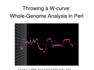
1. Throwing a W­curve:
Whole­Genome Analysis in Perl
●
Steven Lembark <slembark@cheetahmail.com>
http://www.bioinformatics.org

2. A short description of the W­curve
whole­genome comparison project
●
A really quick description of why genome comparison is
useful and messy – and why the W­curve is interesting.
●
How I adapted a graphical display algorithm to make use of
Perl and BioPerl.
●
A few tricks for bulk data analysis in Perl: triangular
comparison using stable metrics and hash slices from
integer sequences.

3. One of the biggest advances in
science was sequencing genes.
●
Genes provide the blueprint for life, and are the core of new
medicine and technology.
●
Drugs are being developed to cure diseases where only
symptoms could be treated before.
●
Bioinformatics is core of a new kind of biology that can
process genetic information in ways unimagined only 10
years ago.

4. We did not evolve to be computable.
●
Comparing genes is difficult.
●
Genes are written in called our DNA as sequences of
“bases” labeled “C”, “A”, “T” and “G”.
●
The genes mostly generate proteins, which are made of
twenty amino acids.
●
The genetic code is redundant and varies even within an
individual; there is “junk” between the genes and within
them; along with variable “repeat” groups.

5. Redundant Coding
●
The triplets are called Leu
Arg
L
R
UUA,
CGU,
UUG,
CGC,
CUU,
CGA,
CUC, CUA, CUG
CGG, AGA, AGG
“Codons”, and actually
Ser S UCU, UCC, UCA, UCG, AGU, AGC
Val V GUU, GUC, GUA, GUG
Pro P CCU, CCC, CCA, CCG
encode RNA (with Ala A GCU, GCC, GCA, GCG
Thr T ACU, ACC, ACA, ACG
bases of C, A, G, & U). Gly G GGU, GGC, GGA, GGG
Ile I AUU, AUC, AUA
Lys K AAA, AAG
●
The 64 combinations of Asn N AAU, AAC
Asp D GAU, GAC
RNA encode only 20 Phe F UUU, UUC
Cys C UGU, UGC
protein building blocks. Gln
Glu
Q
E
CAA,
GAA,
CAG
GAG
His H CAU, CAC
●
This makes “equality” a Tyr Y UAU, UAC
Met M AUG
slippery question Trp W UGG
between genes. Start AUG, CUG, UUG, GUG, AUU
Stop UAG, UGA, UAA

6. What a difference a base makes...
●
The difference between Normal and
Sickle Cell Hemoglobin is caused
by a point mutation: one differing
DNA base changing an amino
acid. Normal
gtt cat tta
Sickle Cell
gtt gtt tta
gtc cac tta gtc gtg tta
●
Replace any sequence on the left gta cat tta gtg gtt ctc
gtc cac ttg gtt gta cta
with any on the right and you gtg cat ctc gta gta tta
gtt cac cta gtg gtg ctg
have Sickle Cell Anemia. gtg cac ctg gtc cac ttg
gta cac ctt gta gtt ctt
●
This difference is among 450_000 ...
bases.

7. Exonic DNA and repeats
●
Much of our DNA produces RNA that is edited out before
protein transcription.
●
Exons are the DNA sequence that actually encodes a
protein.
●
Even “standard” exonic genes have bits of extra material in
them called repeats: O, A, B blood types happen because
varying number of repeated “TA” sequences cause
slightly different proteins to result.
●
This means that two “normal” copies of hemoglobin may
also differ only by having multiple copies of some filler
DNA.

8. Whole­Genome Comparisons
●
Evolutionary biology and drug research both try to
compare all of one organism to another in search of
commonality for evolutionary history or odds that a
disease or cure may be common to the species.
●
This adds to our problems the variability between species
along with all of the within­species (or individual)
variation I've shown so far.
●
People have two hemoglobin genes, which can vary
between them: genome comparisons also most
accommodate variances within individuals.

9. Not quite a consensus
●
For comparing textbook genetics, the “Consensus”
sequence helps remove some variability.
●
This only helps when comparing reviewed sequences that
have one: newly discovered sequences or the raw output
of sequencing equipment will be in whatever order the
organism really has – with all of its variability intact.
●
In fact, one use of these comparison techniques is
determining if different encodings are simply variations
on the consensus.

10. Comparing Genes
●
Our bodies gracefully deal with variability in genes
thousands of times a second; unfortunately for
Bioinformatics, computers deal with this much more
slowly.
●
The common approaches to comparing genes are
Alignment, Hidden Markov Models, and Graphical.
●
Alignment uses recursive algorithms to find what does
match; HMM's look at probabilities that they match;
graphical models map the problem onto something that
supports approximation.

11. Traditional gene matching:
Alignment
●
Traditional method is alignment: BLAST & FASTA are the
standards here.
●
They line up the portions of the sequence, leaving gaps as
necessary.
●
Recursion necessary to shift the mapped portions makes
these slow and them to a few thousand bases.
●
Alignment studies require significant manual intervention
to set up the comparison process.

12. Waiting in line for a gene:
Hidden Markov Models
●
Hidden Markov Models (“HMM”) generate a state
transition model from one set of DNA used to train a
model, then estimate the probability that another
sequence is from the same family.
●
These are slow to train and exquisitely sensitive to the
choice of DNA sequence used for training.
●
They may require more DNA sequences for training than
are readily available, leading to small­sample error or
skewed results.

13. Graphical Models
●
Graphical models abstract the genetic code into some n­
dimensional space for comparison. Geometric algorithms
can then be used to analyze or compare the curves.
●
These are largely intended to use the human brain to
perform the comparison.
●
3D models add dimensions that allow for approximate
results and greater freedom in the algorithms used to
compare genes.
●
The W­curve uses a 3D model, with a simple state machine
generating the curves.

14. The W­Curve Code
●
The original layout was designed by a Java programmer for
use in displaying DNA for visual comparison.
●
It was slow and nearly useless for computed comparison.
●
My job was to fix it using – of course – Perl.
●
The rest of this talk describes what I went through, both in
Perl and the algorithm itself, to get a workable
comparison technique.

15. The W­Curve Algorithem
●
The basic design is a state machine crawling down the
DNA sequence.
●
Each corner of a square is associated with one type of DNA
base.
●
The curve is generated by moving from the current location
half way to the corner associated with the next base.

16. Improving the W­Curve
●
First thing I had to do was find a measure amenable to
comparing the curves; then improve the algorithm for
computing them.
●
Our goal was to find a fast process for whole­genome
comparison.
●
This meant being able to load DNA, generate curves, and
compare them quickly without manual intervention.
●
The result described here is an fast, heuristic utility which
can be developed to perform more exact comparisions
with different measures.

17. Approximate Mesure
●
The comparison rules must accommodate
small differences between sequences.
●
I used the difference along the longer
vector's length: this ignores small
differences and adds the two lengths
when the vectors point in opposite
directions (A > 90 degrees).
●
The measure for comparing two genes is
the average of their differences over the
length of the longer gene with [0,0] filler
on the shorter one.

18. Computing the W­curve
●
Now all I had to do was compute and compare the curves
quickly enough.
●
This involved changing the coordinate system to
cylindrical, redesigning the state­box, hashing the
computed curves by length, and finding efficient ways to
compare the arrays.
●
I also took into account some knowledge about the DNA,
including the need to differentiate AT­ and CG­rich
regions of a sequence.

19. Cylindrical Co­ords
●
The original cartesian co­ordinates made half­intervals easy
to compute but complicated computing the difference
measure.
●
Changing the code to use cylindrical notation (r, angle, Z)
simplified comparing the curves, but left the distances
computed using the square root of two (distance of origin
to (1,1)­style corners).
●
This would have caused significant accumulated error
along the full length of a gene.

20. Initial fixes: Modify the Curve
●
Rotating the square so that it's corners were on the axis
simplified the computations and avoided the rounding
error.
●
Putting A­T and C­G on common edges leaves the curve less
likely to hug the origin.
●
The angle to a corner (“A”) is simply a matter of adding
multiples of PI/2 from a table.
●
The half interval to a corner is simply: ( 1 + r1 * cos(A) ) /
( 2 * cos(A/2) ) with a simple check for 2 * cos(A/2) == 0

21. Next: Computing Curves in Perl
●
Single curves can easily be stored as arrays, the catch is
finding efficient ways to generate them.
●
Given an array of DNA and another of W­curve, one of
them can be handled via for­loop iterator, but the other
requires an index or a shift to walk down.
●
C handles these situations via pointers; Perl requires a bit
more finesse.

22. Compute w­curves in place
●
The good news was that once a W­curve point was
computed its DNA base was used up and could be
discarded.
●
This left me able modify $_ with the result of computing on
$_ to construct the curves in place. This code replaces
each letter of the DNA sequence with its curve point:
my @curve = split //, $dna;
my $state = [ 0, 0 ];
$_ = generate_w_curve $state, $_ for @curve;
$seqz{ $name } = @curve;

23. Comparing Lengths: Arrays
●
Another issue was comparing genes in groups by length.
Genes with base counts (or DNA string lengths) more
than 10% different will rarely be the same gene.
●
The simple approach is to store them by length in an array:
push @{$curvz[$len]}, $curve;
●
Access to the lengths would be an array slice of
@curvz[ 0.90*$len .. 1.10*$len ];
●
Problem here is dealing with a long (Hemoglobin is
450_000 bases) sparse array.

24. Comparing Lengths: Hashes
●
Large, sparse lists are better handled by hashes.
●
This left me with
@curvz{ (0.90*$len .. 1.10*$len ) }
●
Using a numeric range operator to generate hash keys
works just fine: Perl will happily convert your numeric
lists into strings for hash access.
●
That leaves me with nested hashes of ref's to scalars. The
outer key is a length, the inner key a gene name, the leaf
value a w­curve.

25. Upper­triangular comparisons
●
If A == B imiplys B == A, only half of the comparisons
need to be made.
●
The issue for W­curves was making sure that the same
comparison was done regardless of the curve order.
●
Instead of comparing the length of the first curve I ended
up using the longer one to compute the measure, with
[0,0] filler in the shorter curve.
●
This left me with
@curvz{ $len .. 1.1 * $len }

26. Now all I needed was DNA...
●
Genbank­format files have full genomes but are
complicated to parse – their format is regex­proof.
●
Bioperl (and Lincoln Stein ) solved that one for me, using
IO objects.
●
The main problem with Bioperl is – due to parallel
development with other Bio* packages – it looks way too
much like Java in many cases; down to the point of
requiring 3­4 opaque objects to do anything, each of
which has its own fairly opaque documentation.
●
In the end I was able to read each .gbk file and write its
genes back out in FASTA format for comparison.

27. Extracting data from .gbk files
sub read_genome
Bio::SeqIO handles
{
● # grab a copy of the local genbank file
# as a Bio::SeqIO. the only useful thing
the guts of a #
#
from it are the features whose primary
tag is a gene.
Genbank file use Bio::SeqIO;
gracefully. my @seqargz
= ( qw( -format genbank -file ), shift );
●
The result is a species my $fh = Bio::SeqIO->new( @seqargz);
my $seq = ( $fh->next_seq )[0];
name followed by my ( $species )
an array­ref feature = $seq->{species}->common_name
=~ m{^(S+s+S+)};
objects. (
$species,
[
grep { $_->primary_tag eq 'gene' }
$seq->get_SeqFeatures
]
)
}

28. Extracting the ID and Sequence
sub gene_sequences
What I need from
{
● # first step: slurp the genes only.
the objects are my ( $species, $genome )
= read_genome shift;
the gene name # now map the names onto their sequences.
# caller gets back anonymous hash of the
and exonic # gene names mapped onto their sequences.
(“spliced”) DNA.
my $gene_seqz =
{
map
{
●
Once they were (
$_->get_tag_values('gene'),
extracted the )
$_->spliced_seq->seq
BioSeq object
}
@$genome
};
could be # at this point the genome and SeqIO objects
discarded.
# can be discarded: all we need going
# forward is the the text handed back here.
( $species, $gene_seqz )
}

29. Output as FASTA
for my $path ( @ARGV )
●
The the outer loop {
# snag the species name and dna string.
simply cycles the my ( $species, $genome )
= gene_sequences $path;
Genbank files, ( my $base = $species ) =~ s/s+/_/g;
writing out each while( my($gene,$seq) = each %$genome )
gene as a FASTA
{
my $path =
“$Bin/../var/$base.$gene.fasta";
file. open my $fh, '>', $path;
●
Aside: this can # matching on 1,80 char's breaks the long
# string up into separate lines; newlines
# via $,
easily be forked print $fh
by input file. “> $input, $species, $gene",
'',
$seq =~ /.{1,80}/g;
}
}

30. Example FASTA output
●
The resulting FASTA file has minimal information on the
'>' line, with the file sorted by size for more efficient
processing:
> U00089.gbk, Mycoplasma pneumoniae, yfiB
ATGCAAGATAAAAACGTCAAAATTCAGGGCAATCTGGTACGGGTACACCTTTCGGGATCGTTTCTGAAGTTCCAGGCAAT
TTACAAGGTGAAAAAGCTGTACTTACAGCTGTTAATTCTCTCCGTGATTGCCTTCTTTTGGGGCTTGTTAGGAGTTGTGT
TTGTCCAGTTTTCTGGATTATATGACATTGGCATTGCTTCCATTAGTCAGGGCTTAGCACGGTTAGCGGATTATTTAATT
AGGTCGAACAAGGTCAGTGTGGATGCTGACACCATTTACAACGTCATCTTCTGGTTGAGTCAAATTCTGATTAACATTCC
CTTATTTGTTTTGGGTTGGTACAAGATTTCCAAAAAGTTTACCTTGTTAACCCTTTACTTTGTGGTAGTCTCCAACGTTT
TTGGGTTTGCCTTCTCTTACATTCCGGGCGTGGAAAACTTCTTCTTGTTTGCTAATTTAACTGAACTTACTAAGGCCAAC
GGTGGCTTAGAACAAGCGATTAACAACCAAGGGGTGCAACTGATCTTTTGGGAACAAACCGCTGAAAAGCAAATTTCGTT
AATGTTCTATGCGCTGATCTGGGGTTTTCTTCAAGCTGTGTTTTACTCAGTTATCCTAATTATTGATGCATCGAGTGGTG
GGTTGGACTTTTTGGCCTTCTGGTATTCGGAAAAGAAACACAAGGACATTGGTGGTATTTTGTTTATTGTTAACACCCTT
AGTTTCTTGATCGGTTACACCATTGGCACTTACCTTACCGGTAGCTTACTAGCACAAGGCTTTCAAGAAGATAGACAAAA
ACCGTTTGGAGTGGCTTTTTTCTTGTCCCCTAACTTAGTGTTTACGATTTTCATGAACATTATCTTAGGGATCTTTACCT
CCTACTTCTTTCCTAAATACCAGTTTGTCAAAGTGGAAGTGTATGGTAAACACATGGAACAAATGCGCAACTACTTGTTG
AGCAGTAACCAGTCCTTTGCGGTCACTATGTTCGAAGTGGAAGGGGGGTACTCGCGCCAAAAGAACCAGGTGTTAGTTAC
AAACTGTTTGTTTACGAAAACGGCCGAACTTTTAGAAGCTGTTAGACGAGTCGATCCGGATGCTCTGTTCTCAATTACCT
TCATTAAAAAGTTGGATGGTTATATCTATGAAAGAAAAGCACCTGATAAAGTAGTCCCACCA
GTAAAAGACCCAGTTAAAGCCCAGGAAAATTAA

31. Storing DNA for comparison
●
Catch: the whole genome of anything more than bacteria
won't fit into memory at one time.
●
Since I didn't need all of the DNA in memory at once, so I
could store a hash of { length }{ geneid } that was false
until it was first processed, setting
ref $_ || $_ = generate_curve $_
as each item was being processed.
●
I was also able to delete used­up lengths as they
were processed.

32. Performing the comparisons
●
Back to the issue of iterating two arrays again.
●
Linked lists are not used often in Perl but this is one case
they really apply: advancing the two nodes requires only:
( $node, $r, $a ) = @$node
●
The only other issue was avoiding rounding errors
computing 2*cos($a/2).
●
At the edge of precision the value can be non­zero but still
yield essentially infinite results.
●
The fix was to set the value using:
$value = 0 if $value < $TINY;

33. Result: W­curve output
For comparison: This took 45 hours of computing time to validate with FASTA at NIH.
Whole Gnome Comparison:Mycoplasma genitalium, Mycoplasma pneumoniae
Curve Description:
Curve Used: WCurve with T A G C
Score Cutoff: 0.3
Length Cutoff: 0.15%
Report Size:
Base Genes: 480
Matched Base genes: 72 15%
Report Rows: 72 15%
Filter Efficiency:
Cartesian Product: 330240
Alt. Genes Compared: 28851 8.73%
Total Comparisons: 44020 13.32%
Time Efficiency:
Elapsed time: 565 sec
Comparison Time: 558 sec 98%
Comparison Rate : 78 Hz
Results By Gene
Row Mycoplasma genitalium Mycoplasma pneumoniae Score
1 MG325 rpmG 0.158080075467006
2 MG362 rplL 0.176481395732838
3 MG451 tuf 0.185903240607304
4 MG197 rpmI 0.204703167254187
...

34. Summary: Perly Data Handling
●
You may not need all of the data in memory all of the time.
●
Breaking I/O up into chunks often helps: multiple page­size
reads are more efficient than a single large slurp.
●
Pre­process data saves sorting, chunking during processing.
●
Symmetric tests cut the number of comparisons by half.
●
Use $_ to replace data in place rather than store both inputs
and outputs.
●
Look at your computations: simply rotating a box can help.