This article presents the discrete event simulation developed with Northwestern University to optimize an injector production line. This article was presented at the recent Winter simulation Conference (held in December 2008)

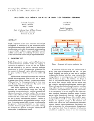
1. Proceedings of the 2008 Winter Simulation Conference
S. J. Mason, R. R. Hill, L. Moench, O. Rose, eds.
USING SIMULATION EARLY IN THE DESIGN OF A FUEL INJECTOR PRODUCTION LINE
Mustafa H. Tongarlak Laurent Borne
Bruce Ankenman Kyle Wolfe
Barry L. Nelson
Delphi Corporation
Dept. of Industrial Engr. & Mgmt. Sciences Rochester, NY, U.S.A.
Northwestern University
Evanston, IL, U.S.A.
ABSTRACT
Delphi Corporation decided to use simulation from concept Subassemblies
development to installation of a new multimillion dollar
fuel injector production line. In this paper we describe how
Cartridge Injector Calibration
simulation was employed in the concept development phase
Assembly Assembly & Test
to assess whether production targets required for financial
viability were feasible and to identify the critical features
of the line on which to focus design-improvement efforts.
Injector
1 INTRODUCTION
Delphi Corporation is a major supplier of fuel injectors
to auto manufacturers around the world. The company is Figure 1: Proposed fuel injector production line.
considering a proposal for a new line that will produce
the next generation of fuel injectors. There are ambitious
requirements on the line’s throughput that are essential for A simulation model and study was commissioned at
the project to be financially viable, and real constraints on a very early stage of designing the new line. The goal
the space available for the line and the cost to build it and for the simulation was to serve as a test bed for candidate
staff it. production-line designs, both from initial concept to fine
As envisioned, this new production line will consist of tuning and even to examining process-improvement ideas
multiple process segments, three of which will be placed after the line is in place. To simulate a line design it
in a clean room. Figure 1 displays a rough representation must be fully specified including which machines to use
of the new line. The three segments inside the clean room and in what order, conveyor lengths, machine process rates
were the main focus of our study since they are the most and variability, operator responsibilities and priorities, and
complex, highly automated and costly. failure and repair distributions for each machine, as well as
Each process segment may contain as many as thirty scrap and rework rates on a machine-by-machine basis. Such
machines and robots performing various tasks along ac- complete and detailed information is typically not available
cumulating conveyors that convey partially completed fuel at the concept stage of the line design, but this is precisely
injectors from machine to machine in pallets. The conveyors when simulation can be most valuable in helping Delphi to
will also act as buffers since they accumulate pallets in front assess whether the project is financially viable and where
of a machine if it is either down or unable to keep up with in the evolving line design the most effort should be spent.
the flow of pallets from upstream machines. Transfer of Using simulation at such an early stage requires making
assembled fuel injectors between process segments will be frequent and significant changes to the simulation base
done via trays that are stacked in carts and moved manually model which can be both time-consuming and difficult to
by operators. Because contamination is a major concern manage. However, the recommendations from the study are
inside the clean room, parts will be washed before entering often inexpensive or free to implement since the equipment
the clean room and operators are assigned tasks that do not has not yet been built. Once the equipment is built, using
require them to move between rooms. simulation to analyze the process is less time-consuming

2. Tongarlak et al.
because establishing the base model is not a moving target. and expand throughout the project, a link was established
The drawback to this approach, however, is that much of between the MSD and the simulation model so that the
the cost is already sunk and the recommendations from the simulation would always be run with the most up-to-date
study may be more difficult to cost-justify. This was our data.
challenge. However, the MSD was more than just a data source; it
Notice that it makes no sense early on to try to optimize was also used to balance the line to produce k fuel injectors
the design over the literally hundreds of changeable features every minute (where k was a value set by Delphi and will not
because too little is known and too much is in flux. Instead, be revealed here). In this semi-automated system where a
simulation was exploited to answer high-level questions series of processes are connected to each other, “balancing”
about the line configuration, with the understanding that simply means that if a particular operation is not able to
the model would later evolve into a representation capable produce the target k parts per minute then enough parallel
of evaluating very specific questions. That is, the simula- capacity is added to keep up with the production requirement.
tion was first to guide the development of new designs by Since the line will operate for 24 hours/day, the production
distinguishing critical features and factors from less-critical capacity of the line would be 1440k parts/day if there were
ones, and later to be updated as new designs emerged. In no machine downtimes, no scrap, no process variability and
this way the simulation would provide a perpetual road map material buffers would never go empty. However, to bring
for next steps in the design process. This paper is a product more realism, the MSD also incorporated discount factors
of the first phase (about 6 months) of this iterative design for percentage of scrap and downtime by machine, leading
process where answering high-level questions about line to a still optimistic throughput target of 1125 k fuel injectors
configuration, conveyor layout, and operator assignments per day, or approximately 22% less than the theoretical
was of primary concern. In this way we will illustrate how maximum. Achieving this target is necessary for the new
simulation can have a profound impact at the concept stage fuel injector project to be financially viable.
of a complex project. The reason that 1125k fuel injectors per day may be
optimistic is that a static analysis such as the MSD provides
2 SYSTEM DESCRIPTION AND DATA SOURCES cannot account for the impact of process variability, starva-
tion due to lack of material or blocking, operator response
Clearly machines (including robots) and conveyors need time to failures, conveyor congestion, etc. More accurate
to be included in the simulation model. Most machines analysis of the proposed system requires the fidelity of a
will keep running until a failure occurs as long as they detailed simulation model which takes into consideration
are not starved or blocked. Since conveyors will be han- the interactions among all parts of the system as well as
dling the subassemblies within process segments, operators randomness inherent to the system. The critical question
are needed only for transferring assembled fuel injectors to be answered by the simulation at the concept stage was
between process segments, filling raw material buffers, re- whether 1125k fuel injectors per day was actually feasible
pairing machines and periodically performing other tasks and what it might take to get there.
such as quality checks, rejected fuel injector handling and In the following subsections we list some of the key
preventative maintenance. Even though the system is semi- system elements that figured in our analysis and mention
automated and operators are only lightly involved with actual any approximations we made.
operations, their supporting role in the system is critical be-
cause machine failures will occur, and input buffers will 2.1 Resources
be consumed, leading to lost production if operators are
unable to keep up. Therefore, in addition to machines and Each machine is prone to failure and the average time it
conveyors, operators, injector trays and material carts were runs until a failure occurs is represented by a Mean Time
included in the model. Before Failure (MTBF). Once it fails, a machine waits for
Delphi represented line designs as AutoCAD drawings the appropriate operator to come and fix it. The time it
(that eventually became backgrounds for the simulation takes for an operator to arrive and then repair the machine
animation). More importantly, Delphi also maintained a is downtime when no parts can be produced. The average
single Excel spreadsheet with many worksheets called the repair time is denoted by Mean Time To Repair (MTTR).
Manufacturing System Design (MSD) that always contained The MTBF and MTTR are values derived from information
the current state of knowledge about the line design. This in the MSD, and the distributions of the time to failure and
included process information of all types, from raw material repair were modeled as exponential.
buffer sizes and operator task assignments to anticipated
machine reliabilities, processing times and processing-time
variabilities. Since this information ranged from firm values
and commitments to educated guesses, and would evolve

3. Tongarlak et al.
Operator
2.2 Operators Arrives
There are three types of tasks that need operators: Machine
!quot;
Attention (MA) Tasks, Periodic (P) Tasks, and Material
Handling (MH) Tasks. Each type of task requires a different #
#
set of skills. MA tasks have the highest variability while Operator
#
MH tasks are the most regular. Therefore, operators will not Leaves
be assigned both MA and MH tasks. However, all operators
will have some P tasks they need to perform like quality
checks, reject handling and maintenance tasks.
P tasks need to be done regularly every 2, 4, 8, 24, or
120 hours. MH tasks—much like P tasks—are performed
periodically but are more frequent than P tasks. However, Figure 2: Flowchart of operator tasks.
when P tasks do occur, they have priority over MH tasks.
On the other hand, MA tasks are done as needed; i.e., if an
operator is responsible for fixing a certain machine, then is repaired first if both 5 and 3 are failed. One way that
they only attend to this duty once that machine fails. Mostly priorities arise is that the failure of a unique machine is
because of this random nature of MA tasks, allocation of jobs given priority over repair of one of a number of parallel
to operators is challenging and poor operator assignments machines.
can hamper productivity. For example, suppose that a
certain operator is responsible for repairs on both machine 2.3 Process Variation
A and machine B. If machine A fails, the operator will
respond to that machine as soon as possible. However, if Each machine has an average processing time given in
machine B fails while machine A is still being repaired, its specifications. Because some level of variation exists
the actual downtime of machine B will include not just its in processing rates, it is not possible to produce k fuel
own repair time, but also the remainder of the time it takes injectors every minute even when no scrap is produced and
the operator to complete the repair of machine A and any no machine is down. Since process variation is a factor
travel time between the two machines. In general, operators affecting production, it needs to be embedded in the model.
can be responsible for repairs on many machines so this With help from the Delphi production team, we classi-
effect can be multiplied many times causing substantial fied the process variation of each machine into one of the
downtime. Thus, to whatever extent possible, the MA and following three categories based on their knowledge of the
P tasks should be balanced among the qualified operators process: High, Medium and Low Variation. We assigned a
so no single operator is responsible for repair on more coefficient of variation (CV) for each of these categories. CV
machines than necessary. To define a base case for operator is defined as the ratio of the standard deviation to the mean.
assignments, each MA and P task was assigned to only Since the mean process time was specified, we could then
one of the operators, the tasks were grouped by proximity calculate the process standard deviations through these CV
and then were approximately balanced taking into account values. Using this mean and standard deviation, we spec-
the relative reliability of the machines. All MH tasks were ified a normal distribution to generate random processing
assigned to an operator who handled no MA or P tasks. times for each part processed by that machine.
An extensive point-to-point walk matrix was developed to
accurately account for operator travel times. 3 SIMULATION MODEL
Figure 2 is a flowchart representation of the logic used
in the simulation model for operator activity. Each operator The simulation model was developed in version 12.00 of
is given responsibility for performing certain tasks; as soon the Arena simulation software (Kelton, et al. 2006). This
as an operator completes a task they seek another one unless software by Rockwell Automation was a good choice for
they have completed their shift or it is time for lunch or a the project for the following reasons:
break. Lunches and breaks have priority over tasks. Among
• Arena is well-suited to modeling conveyors. In
the three types of tasks, the highest priority is given to MA
Delphi’s production lines, conveyors are the major
tasks, since if a machine is down then filling buffers or
mode of material transfer.
handling rejects instead of fixing the machine is considered
• Arena provides a user-friendly interface that makes
a bad use of operator time. Also, if two tasks of the same
understanding and modifying the model easier for
type become due or call for attention, then there is a fixed
people other than the modeler. In addition, it
priority order. For example, if operator 4 is responsible
gives the ability to create templates through which
for repairing resources 5 – 3 – 4 – 6 in that order, then 5

4. Tongarlak et al.
similar code can be created for the parts of the line design as specified in the MSD; and the target of 1125k
model that are likely to be repeated with different fuel injectors per day. If there had been no gap between
parameters. For instance, we designed a template these two, then the proof-of-concept phase of the line design
that handles the tasks performed when a part arrives would be done. Instead, there was a very substantial gap, so
to a machine to be processed, such as picking the the objective became finding the key factors that produce the
part from the conveyor, checking for raw material gap so that they can become the focus of future design efforts.
inventory, processing the part and placing the part This must be done without specific design alternatives with
back to the conveyor. Once the template is created, which to compare, which led to the experimental approach
a modeler only needs to define machine-specific described below. The critical factors were unexpected, but
parameters like conveyor name, machine number, completely understandable after the fact.
buffer type, etc. and customized code will be
generated automatically. 4.1 First-Phase Scenarios
• The model can be linked to a data source (e.g., the
MSD, an Excel spreadsheet) to allow for making To design our preliminary experiments, called “first-phase
most minor updates (e.g., changing MTBF for some scenarios,” we listed all of the factors—at an aggregate
machines) directly in Excel rather than in Arena. level—that may contribute to the loss of production. Obvi-
This also preserves data integrity since all Delphi ously, if no such factors existed, then we would be consis-
analysis use a common data source. tently producing 1125k fuel injectors per day. The following
• Arena provides animation capability that can be are some of the factors we listed as potentially critical: Pro-
used for model validation and demonstration pur- cess variability, scrap rates, failure and repair rates, operator
poses. assignments, conveyor lengths, and number of pallets on
• Arena collects and reports most of the necessary each conveyor.
statistics by default and lets the modeler add other The first three scenarios that we studied were selected
statistics. to quantify the effects of process variability, scrap rates,
and repair times. Since each machine has a specified scrap
4 SIMULATION EXPERIMENTS AND RESULTS rate, variability and repair time, there are literally hundreds
of combinations that could be tested. At 8 hours per test, it
The main performance measure in our simulation study was would be impossible to test the impact of these individual
long-run average daily fuel injector throughput; i.e., the long- changes. However, since we are primarily interested in
run average number of fuel injectors that can be produced broad questions about the effects that have the biggest im-
in a 24 hour period. Therefore, we treated this as a steady- pact on throughput, we grouped the potential changes into
state simulation (Banks et al. 2005) requiring a so-called functional categories. For example, instead of investigating
“warm-up period” to get from the initial state (system empty, each machine’s process variability individually, we investi-
all input buffers full, all machines operational) to long-run gated the effect by eliminating all the process variability;
operating conditions. For the base case (described below) this allows us to quantify the maximum impact that process
approximately one day’s production was adequate, so we variability has on the throughput. We constructed similar
made each replication 11 days long with the output data from scenarios to examine the effects of scrap rates and repair
the first day discarded and 10 days (two weeks) retained. We time. Thus, the first-phase scenarios included:
then made enough replications to estimate long-run average
• Scenario 1: Base case, the model representation
throughput to within 5% relative error, and this required
of the factory as reflected in the MSD file and the
20 replications. To give some idea of the experimental
AutoCAD drawing of the layout.
effort to run one scenario, it takes approximately 8 hours
• Scenario 2: All process variation is removed from
to obtain 20 replications of 11 days on a relatively fast
the base case.
PC. This is a function of both the size and complexity
• Scenario 3: Process variation and all scrap are
of the system, and the very large number of fuel injector
eliminated from the base case.
subassemblies in process at any one time. Since all other
• Scenario 4: Repair times are set to zero; that is,
scenarios are modifications of the base case, we used the
as soon as an operator attends to a failed machine,
same experimental effort (20 replications of 11 days) on
it starts running again and the operator can leave
each of the scenarios tested. Although throughput was
for next assignment.
the driving performance measure, measures of operator
utilization, machine downtimes, congestion on conveyor
Scenario 2, which eliminates the process variation, was
segments, and raw material buffer states were also examined.
especially critical because the variation input to the model
Results from all experiments were compared to two
was based on expert opinion and estimated CV’s. Therefore,
benchmarks: the base case, which is a simulation of Delphi’s

5. Tongarlak et al.
if eliminating all the variation does not achieve a significant returned to the base case scenario and looked at statistics that
production gain, then putting effort into creating better were collected to discover other reasons for lost production.
estimates of CV for the processing time of each machine is There were four types of analysis we were interested in
not essential at the conceptual design stage. If, on the other making: Operator availability, pallet congestion, inventory
hand, it makes a significant difference, then we should not levels, and failure analysis.
make radical design changes before this variation is carefully Operator utilizations in the base case showed all oper-
characterized. ators were heavily utilized. Some operators were so very
Scenario 3 eliminates both scrap and process variation. heavily utilized that they often did not complete their peri-
This scenario was intended to inform us of the sensitivity odic tasks, such as quality checks, during their shift and so
of throughput to scrap rates and to determine if it is critical these tasks were pushed to the following shift. For certain
to improve the estimates of the machine scrap rates before tasks, the operators in subsequent shifts were also too busy
proceeding. The purpose of eliminating both process vari- to complete these tasks and thus it was clear that these types
ation and scrap rate together is to use this scenario as a of jobs would build up and never be completed. An even
“best case scenario” for this design candidate. more significant consequence of having heavily utilized op-
Scenario 4 takes a different approach than 2 and 3. erators is that many machine failures did not get immediate
In this experiment, repair times were set to zero while attention from operators and thus operator response time
scrap and process variation were retained. The goal was to machine failure began to overwhelm repair time as the
to see the potential of the production line when repairs primary cause of machine downtime. This raised the ma-
are done infinitely fast and machines are down only for chine downtimes for most machines far above the expected
the amount of time it takes for the designated operator to downtime and caused dramatic production losses.
attend the machine (i.e., response time, which consists of Another system measure is congestion on conveyors.
time to complete a periodic task in progress and walking A very straightforward way of knowing which conveyor
travel time). When repair times were set to zero, operators segments experience higher congestion is to look at which
become more available and as a result response times to segments are heavily utilized for a long time. Before running
failures also decrease. We recognize that this level of service any of the scenarios, we created 4 utilization states: Fully,
is impossible to achieve but this scenario showed us the Highly, Moderately and Lightly Utilized. Throughout the
benefits of improving machine attention activities. 10 days of each replication, we monitored the amount of
time that each conveyor segment spent in each utilization
4.2 First-Phase Results and Analysis state. Conveyor segments that spent a high percentage of
time in Fully or Highly Utilized states were marked and
For the base case scenario, the average daily production compared to the machine downtimes in the vicinity of these
value estimate was only 800k fuel injectors per day or 71% conveyors. Our conclusion for the base case was that there is
of the target throughput for the new line. This left a gap a very strong relationship between operators not being able
of nearly 30% between planned and realized production. to quickly respond to machine failures and heavy utilization
The results of scenarios 2–4 shed light on what caused of the conveyor segments just upstream of those machines.
this gap and what design changes would give the largest Raw material buffer inventory is also of interest. The
improvement. question is whether there are machines that go idle due
In scenario 2 when process variation was taken out from to lack of material. In all of our scenarios, there was one
all of the machines, daily production relative to the goal operator dedicated to raw material handling and that operator
went up to 75%. In scenario 3, in which both process vari- had no machine repair responsibilities. Thus, this function
ability and scrap were eliminated, this percentage became was not affected by the excessive machine downtime. Our
76%. Both of these drastic and unattainable changes to the conclusion from analyzing inventory buffers was that the
system produced only slight reductions in the production material handling assignments for the base case worked out
gap. Therefore, we concluded that more detailed analysis of very well and needed only minor adjustments.
machine process variation and scrap rates should be left to Finally, some detailed failure analysis was done since
later stages of our study after other more influential changes over utilized operators and highly congested conveyor seg-
were made to the system. ments may be the symptoms of another problem: Fre-
In scenario 4, in which repair times are reduced to zero, quently failed machines. As with the conveyors, statistics
the goal of 1125k fuel injectors per minute was achieved. on percentage of time each machine is Idle, Busy or Failed
In fact the average daily production for this scenario was were collected. Then, for each machine in the system, we
102% of the target. This significant jump from base case compared resulting downtime percentages to the expected
was a good indication that machine downtime is one of downtime from the MSD model. For the majority of ma-
the primary causes of the low production in the base case. chines in the base case, the downtime percentages were 2–3
However, before we jumped to a conclusion too quickly, we times higher than expected (see Figure 3 for a comparison

6. Tongarlak et al.
incorrect for the base case and the approximation for MTT R
15
in (2) is poor.
The first response to this information is that all reason-
able effort should be made to determine a good estimate
Percentage Downtime
of MTTR for each machine so that the base case can be
10
correctly simulated. However, this would require substan-
tial time to carry out data collection at a current production
facility with similar machines, if they could be found. An-
other option, more in the spirit of the use of simulation early
5
in the design process, is to redesign the base case to reduce
the operator load and thus reduce the impact of MORT.
Additional scenarios were used to help to understand the
0
problem of operator loading on the base case and potentially
Input Base case output
suggest new design directions.
4.3 Second-Phase Scenarios
Figure 3: Comparison of input and output downtime per-
centages for a sample machine in the base case.
In light of the results of first-phase scenarios, the second-
phase experiments focused on operator availability for ma-
chine failures. The operator assignments for the base case
of downtime for a typical machine). Thus, we concluded
scenario involved some critical assumptions, some of which
that excessive machine downtime was the primary cause of
may have a substantial impact on daily production numbers.
the 30% gap between the target and the base case scenario.
For instance, in the base case design, each task (a quality
There are three direct contributors to the average ma-
check, a machine repair or a material handling job) was
chine downtime: MT BF, MT T R and mean operator re-
assigned to a specific operator and no other operator on
sponse time (MORT ). Percent Downtime (PD) can be
that shift could respond to that task. As a result, when
calculated as
a particular operator was heavily utilized, failed machines
would often wait for long periods of time before the assigned
PD = 100(MORT + MT T R)/(MT BF + MORT + MTT R).
operator would arrive to start repairs. Similarly, when an
(1)
operator was gone for their lunch or break, any failed ma-
Percent machine downtime for the MSD model was esti-
chine assigned to that operator would have to wait until the
mated by observing current machines that are similar to the
lunch or break was completed before any repair began. In
ones planned for the new production line. Because it directly
this highly connected production system, any deviation of a
affects the production, percent downtime for each machine
machine from its production target is enough to slow down
is often recorded. MT BF for the MSD model is also easily
finished fuel injector throughput.
collected since machines often have runtime monitors on
Another assumption in the base case was that operators
them. However, separating out the operator response time
leave for lunch or break on schedule as soon as the task
from the repair time is not typically done, and would in
at hand is completed. In some cases, this could leave one
fact be very difficult without a lengthy time study on each
or more machines failed through an entire lunch or break
machine. This means that we can easily estimate the sum
period. In addition, all of the operators go to lunch or
of MORT and MT T R, but we cannot estimate either of
break at the same time, further complicating the downtime
them individually. When setting up the base case scenario,
problem. Clearly the throughput gap might be reduced by
this problem came into play since each machine must have
redesigning the lunch and break times of operators, possibly
a distribution specified for both time before failure ( T BF)
cross-training some operators to provide back-up for others,
and time to repair (T T R). As a simplification, we assumed
or by setting the priorities differently regarding lunches and
that if operator assignments were well designed then MORT
breaks or specific machines.
would be substantially less than MTT R and thus negligible.
To quantify the potential of operator redesign, Scenario
Therefore, solving (1) for MT T R we get
5 used the base case, but eliminated lunches and breaks
from operator schedules. This experiment was designed to
MT T R ≈ PD × MTBF/(100 − PD), (2)
determine an upper bound on the production gain that could
be achieved by optimizing the rules on operator lunches
where PD and MTBF are the estimates of percent machine and breaks, while the base case implemented a worst-case
downtime and MTBF from the MSD. Given the results of scenario where lunch and breaks not only have priority,
scenario 4, the assumption that MORT is negligible was but also all occur at the same time. Of course working

7. Tongarlak et al.
operators without any breaks is not realistic, nor is having
15
them all take lunch at the same time. However, the point
of these experiments is not to make a final suggestion
for implementation, but instead to guide the design efforts.
Percentage Downtime
Furthermore, there are practical ways to implement coverage 10
of lunches and breaks, such as adding support operators to
relieve operators when they leave for breaks so all the tasks
are continually done.
The selection of scenario 6 was intended to determine 5
how much the approximation of MT T R in (2) affected the
daily production rate in the base case. Recall that MT T R for
each machine is a direct input to the simulation model. More
0
specifically, each time machine j failed, a random repair Input Base case output MTTR/2 output
time was drawn from an exponential distributionwith a mean
MT T R j , which was calculated from (2) using estimates of
the downtime and MTBF for that machine or comparable Figure 4: Downtime percentages in base case and in the
machines from current production lines. Operator response MT T R/2 scenario compared to input value.
time, on the other hand, is a random output from the
simulation model which depends on the random machine
failures as well as the operator utilization levels. The the operator response time is negligible and investigation
approximation in (2) used for the base case assumes that of the downtime for this scenario still does not match
all of the downtime is repair time and we found this to the expected downtime from current production lines (see
be inaccurate. Scenario 4 went to the other extreme and Figure 4). However, in scenario 6, in which lunches and
assumed that all the downtime was operator response time, breaks are included, but mean time to repair is cut in
which we also know is not true since repairs do take time. half, the throughput is 92% of the target. This indicates
Scenario 6 attempts to split the difference between these that if the MT T R rates were indeed half of the originally
two scenarios and assumes that the repair will account for proposed MT T R rates, then both downtime and production
about half of the downtime and operator response time will rates would nearly meet expectations.
be the other half. Thus, for scenario 6, the MT T R for Caution must be taken in interpreting scenario 6. The
each machine was cut in half. Therefore, the following two operator response time in the simulation model is based
scenarios were run as second-phase scenarios: on the level of operator staffing and their assignments.
Recall that the downtime estimates from current production
• Scenario 5: Full relief of lunch and breaks. This
machines are also based on some level of operator staffing
scenario has lunches and breaks fully staffed with
and some system of task assignment that was not recorded
no reduced efficiency.
(and are not necessarily relevant to the new production
• Scenario 6: Mean time to repair (MTTR) is cut in
line). Thus, the conclusion of this second phase is that
half. This scenario anticipates that about half of
it is vitally important to determine an accurate estimate
the machine downtime is operator response time.
of the MT T R for each machine that is independent of the
operator response time. Only with good estimates of MTT R
In both of these scenarios, the base case assumptions
can accurate estimates of the daily throughput be trusted.
are kept the same except for the changes mentioned. Thus,
Once accurate estimates of the MT T R for each machine are
scrap and process variability rates are included at the same
collected, new design candidates can be accurately tested. In
levels as in the base case.
particular, scenario 5 indicated that substantial increases in
daily throughput can be gained by working out an operator
4.4 Second-Phase Results
schedule that provides task coverage for operators when
they take lunch or breaks.
In scenario 5, where lunch and breaks are fully covered
The results from all six scenarios are summarized in
by relief operators, the expected daily production value
Table 1.
relative to the production target was 85%. Despite substantial
improvement, this shows that even if the base case were
5 CONCLUSIONS
redesigned to provide operators that fully cover the lunches
and breaks, there would still be a gap between the achieved
Many real-world projects provide moving targets as the busi-
production and the target of 1125 k fuel injectors per day.
ness climate, physical and financial constraints and product
However, this scenario is still using the assumption that
concept evolve. This might suggest that simulation, which

8. Tongarlak et al.
of Science degree from the IFP School in Paris, France,
Table 1: Comparison of daily production values. an MBA from the Kellogg School of Management and a
Master of Engineering Management from the McCormick
Daily Production School of Engineering and Applied Sciences at North-
Scenario (relative to target) western University in Evanston, IL. He can be reached
1: Base case 71% at <Laurent.borne@delphi.com> .
2: No Process Variability 75%
3: No PV & No Scrap 76% BARRY L. NELSON is the Charles Deering McCormick
4: No Repair Time 102% Professor of Industrial Engineering and Management Sci-
5: Full Relief Lunch & Break 85% ences at Northwestern University and is Editor in Chief
6: MTTR/2 92% of Naval Research Logistics. His research centers on the
design and analysis of computer simulation experiments
is a detail-oriented methodology, is not suitable for system on models of stochastic systems. His e-mail and web
design until quite late in the development of the manu- addresses are <nelsonb@northwestern.edu> and
facturing system. However, the ongoing use of simulation <www.iems.northwestern.edu/˜nelsonb/> .
by Delphi to design and evaluate their next-generation fuel
injector production line illustrates the value of simulation, MUSTAFA H. TONGARLAK is a Ph.D. student in
even very early in the design process. The key is using the Department of Industrial and Management Sciences
simulation to answer questions at the right level, including at Northwestern University. His research interests
questions about project viability and where to place the include simulation and metamodeling with applica-
most effort in system design. A simulation is capable of tions to manufacturing. His e-mail and web addresses
addressing these needs well before detailed specifications are and
<m-tongarlak@northwestern.edu>
are available. And if the simulation is constructed in a way <users.iems.northwestern.edu/˜mustafa> .
that makes it reasonable to update and refine, then it can
continue to contribute throughout the project lifecycle. KYLE WOLFE is a Senior Industrial Engineer with Delphi
Powertrain Systems in Rochester, NY. He holds a Bachelor
REFERENCES of Science in Industrial and Operations Engineering degree
from the University of Michigan and a Masters of Business
Banks, J., J. S. Carson, B. L. Nelson and D. Nicol. 2005. Administration degree from the University of Michigan-
Discrete-event system simulation. 4th ed. Upper Saddle Flint. He can be reached at <kyle.s.wolfe@delphi.
River, NJ: Prentice Hall. com>.
Kelton, W. D., R. P. Sadowski and D. T. Sturrock. 2006.
Simulation with Arena. 4th ed. New York: McGraw-
Hill.
AUTHOR BIOGRAPHIES
BRUCE ANKENMAN is an Associate Professor in the De-
partment of Industrial Engineering & Management Sciences
at Northwestern University. His research interests include
the statistical design and analysis of experiments. Although
much of his work has been concerned with physical experi-
ments, recent research has focused on computer simulation
experiments. Professor Ankenman is currently the director
of the Masters of Engineering Management Program and
the director of the Manufacturing and Design Engineering
Program. He co-directs the freshman engineering and de-
sign course (EDC), and is the director of undergraduate
programs for the Segal Design Institute. His e-mail and
web addresses are <ankenman@northwestern.edu>
and <users.iems.northwestern.edu/˜bea/> .
LAURENT BORNE is a Project Manager with Delphi
Powertrain Systems in Rochester, NY. He holds a Master