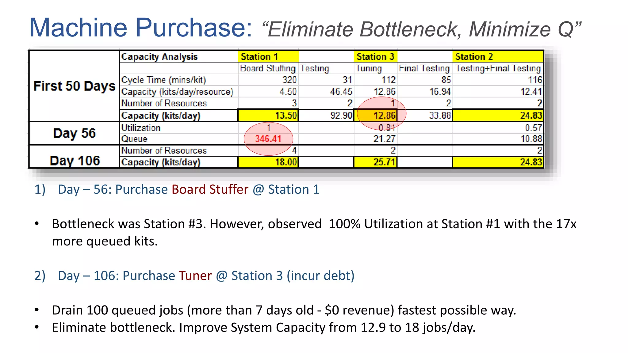
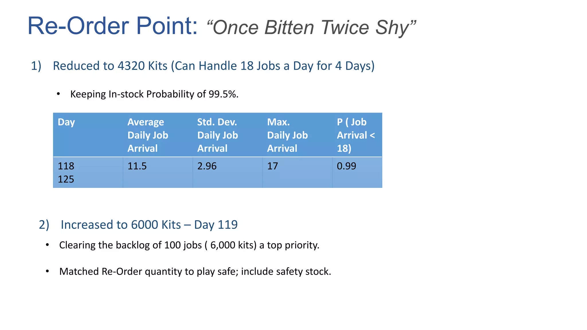
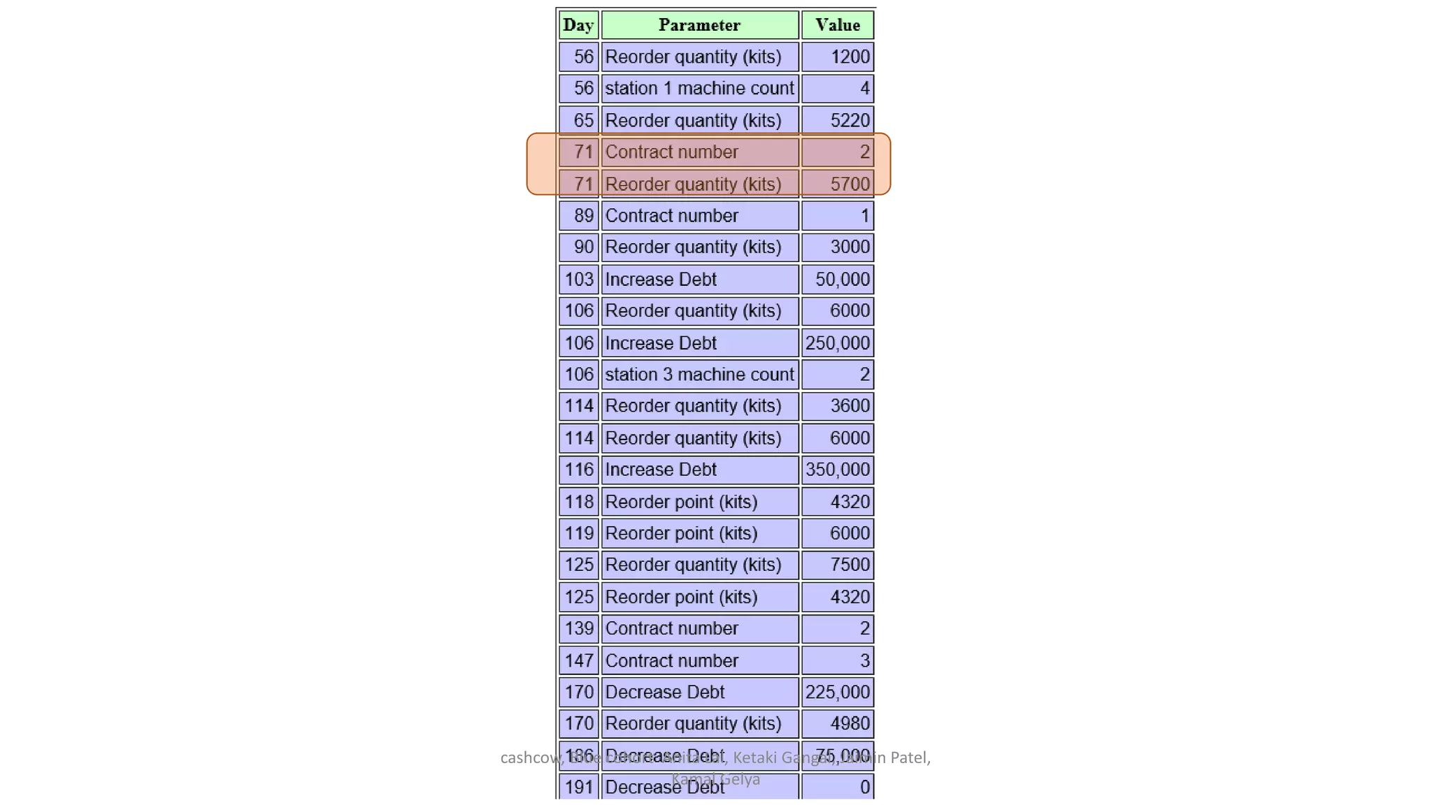
Littlefield Simulation
BLUEs:
Anita Lal
Jaimin Patel
Kamal Gelya
Ketaki Gangal
Machine Purchase: “Eliminate Bottleneck, Minimize Q”
1) Day – 56: Purchase Board Stuffer @ Station 1
• Bottleneck was Station #3. However, observed 100% Utilization at Station #1 with the 17x
more queued kits.
2) Day – 106: Purchase Tuner @ Station 3 (incur debt)
• Drain 100 queued jobs (more than 7 days old - $0 revenue) fastest possible way.
• Eliminate bottleneck. Improve System Capacity from 12.9 to 18 jobs/day.
Re-Order Quantity: “Debt is Cheaper than Stock-Out”
Day Re-Order
Quantity
Cash
Balance ($)
Job Arrival
Rate
Service Job
Rate
Rationale
56 1200 $19,800 12 11.1 Low Cash Balance.
No loan available yet.
Serve Immediate Demand.
65 5200 $68,232 11.5 11.24 Historical average of first 50 days.
Use no more than 75% of cash balance.
125 7500 $98,000 10.7 8.3 Incur Debt.
But use no more than 75% of cash balance.
Re-Order Point: “Once Bitten Twice Shy”
Day Average
Daily Job
Arrival
Std. Dev.
Daily Job
Arrival
Max.
Daily Job
Arrival
P ( Job
Arrival <
18)
118
125
11.5 2.96 17 0.99
1) Reduced to 4320 Kits (Can Handle 18 Jobs a Day for 4 Days)
2) Increased to 6000 Kits – Day 119
• Clearing the backlog of 100 jobs ( 6,000 kits) a top priority.
• Matched Re-Order quantity to play safe; include safety stock.
• Keeping In-stock Probability of 99.5%.
End Game: “Be Risk Averse, Yet Maximize Profit”
1) Choice of Contract: #3
2) Re-Order Quantity: 7500  4980 Kits (Experiment Early - since Day 170)
• Inventory is NOT Cash Balance. Maximize cash balance by minimizing inventory.
System
Capacity
Queue Time Processing
Time
Average Lead
Time
Min.
Revenue
Earned
P (Lead
Time >
0.5 Day)
18 Jobs/Day ~ 0 0.38 Days 0.43 Days 1024 0.05
Re-Order
Quantity
# of Shipments Shipment Cost
($)
Inventory Loss
Potential ($)
Max. Loss
Potential ($)
7500 10 10000 75000 85000
4980 14 14000 49800 63800
4320 17 17000 43200 60200
Littlefield Simulation -
Appendix
Contract Selection Decision
cashcow, Blue cohort Anita Lal, Ketaki Gangal, Jaimin Patel,
Kamal Gelya
Decision Analysis
Day 71: Contract 2 Based on job lead times
Day 89: Contract 1 Little’s Law: Average Flow Time = Average Inventory (day 1-88) / Average Flow Rate
(11.15 kits/day) = 4.13 Days.
Cannot commit 1 day of contract 2. Switched back to contract 1
Day 129: Contract 2 Maximize profit based on system capacity, job arrival and completion rate
Day 147: Contract 3 Maximize profit based on system capacity, job arrival and completion rate
cashcow, Blue cohort Anita Lal, Ketaki Gangal, Jaimin Patel,
Kamal Gelya
cashcow, Blue cohort Anita Lal, Ketaki Gangal, Jaimin Patel,
Kamal Gelya
cashcow, Blue cohort Anita Lal, Ketaki Gangal, Jaimin Patel,
Kamal Gelya
Re-order Point
cashcow, Blue cohort Anita Lal, Ketaki Gangal, Jaimin Patel,
Kamal Gelya

Littlefield Simulation

  • 1.
    Littlefield Simulation BLUEs: Anita Lal JaiminPatel Kamal Gelya Ketaki Gangal
  • 2.
    Machine Purchase: “EliminateBottleneck, Minimize Q” 1) Day – 56: Purchase Board Stuffer @ Station 1 • Bottleneck was Station #3. However, observed 100% Utilization at Station #1 with the 17x more queued kits. 2) Day – 106: Purchase Tuner @ Station 3 (incur debt) • Drain 100 queued jobs (more than 7 days old - $0 revenue) fastest possible way. • Eliminate bottleneck. Improve System Capacity from 12.9 to 18 jobs/day.
  • 3.
    Re-Order Quantity: “Debtis Cheaper than Stock-Out” Day Re-Order Quantity Cash Balance ($) Job Arrival Rate Service Job Rate Rationale 56 1200 $19,800 12 11.1 Low Cash Balance. No loan available yet. Serve Immediate Demand. 65 5200 $68,232 11.5 11.24 Historical average of first 50 days. Use no more than 75% of cash balance. 125 7500 $98,000 10.7 8.3 Incur Debt. But use no more than 75% of cash balance.
  • 4.
    Re-Order Point: “OnceBitten Twice Shy” Day Average Daily Job Arrival Std. Dev. Daily Job Arrival Max. Daily Job Arrival P ( Job Arrival < 18) 118 125 11.5 2.96 17 0.99 1) Reduced to 4320 Kits (Can Handle 18 Jobs a Day for 4 Days) 2) Increased to 6000 Kits – Day 119 • Clearing the backlog of 100 jobs ( 6,000 kits) a top priority. • Matched Re-Order quantity to play safe; include safety stock. • Keeping In-stock Probability of 99.5%.
  • 5.
    End Game: “BeRisk Averse, Yet Maximize Profit” 1) Choice of Contract: #3 2) Re-Order Quantity: 7500  4980 Kits (Experiment Early - since Day 170) • Inventory is NOT Cash Balance. Maximize cash balance by minimizing inventory. System Capacity Queue Time Processing Time Average Lead Time Min. Revenue Earned P (Lead Time > 0.5 Day) 18 Jobs/Day ~ 0 0.38 Days 0.43 Days 1024 0.05 Re-Order Quantity # of Shipments Shipment Cost ($) Inventory Loss Potential ($) Max. Loss Potential ($) 7500 10 10000 75000 85000 4980 14 14000 49800 63800 4320 17 17000 43200 60200
  • 6.
  • 7.
    Contract Selection Decision cashcow,Blue cohort Anita Lal, Ketaki Gangal, Jaimin Patel, Kamal Gelya Decision Analysis Day 71: Contract 2 Based on job lead times Day 89: Contract 1 Little’s Law: Average Flow Time = Average Inventory (day 1-88) / Average Flow Rate (11.15 kits/day) = 4.13 Days. Cannot commit 1 day of contract 2. Switched back to contract 1 Day 129: Contract 2 Maximize profit based on system capacity, job arrival and completion rate Day 147: Contract 3 Maximize profit based on system capacity, job arrival and completion rate
  • 8.
    cashcow, Blue cohortAnita Lal, Ketaki Gangal, Jaimin Patel, Kamal Gelya
  • 9.
    cashcow, Blue cohortAnita Lal, Ketaki Gangal, Jaimin Patel, Kamal Gelya
  • 10.
    cashcow, Blue cohortAnita Lal, Ketaki Gangal, Jaimin Patel, Kamal Gelya
  • 11.
  • 12.
    cashcow, Blue cohortAnita Lal, Ketaki Gangal, Jaimin Patel, Kamal Gelya