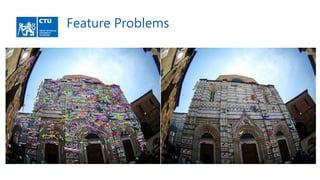
Download to read offline

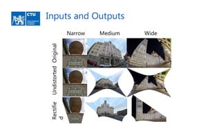
![Solver Variants Generated
Reference [1] Proposed Minimal Solvers [2] [3] [4]
Undistorts ✓ ✓ ✓ ✓ ✓
Rectifies ✓ ✓ ✓ ✓ ✓ ✓
# points 2 2.5 3 3.5 4 4 5 5
Directions 1 1 1 2 2 2 1 1
# solutions 1 4 2 6 4 1 18 5
• One and two-direction variants of the proposed solvers are in colors.
• Each variant has a version that can rectify reflections (green, blue).](https://image.slidesharecdn.com/rdct-180718143111/85/Radially-Distorted-Conjugate-Translations-8-320.jpg)
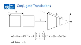
![Comparison of Generated Solvers
z Original
(dashed)
Hidden
(solid)
80x84 14x18
74x76 24x26
348x354 54x60
730x734 76x80
Solvers based on constraints using the hidden variable trick are smaller and
more stable than solvers generated using [5] with the original constraints.](https://image.slidesharecdn.com/rdct-180718143111/85/Radially-Distorted-Conjugate-Translations-16-320.jpg)
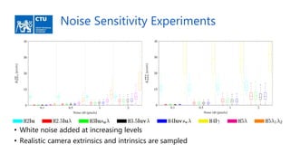


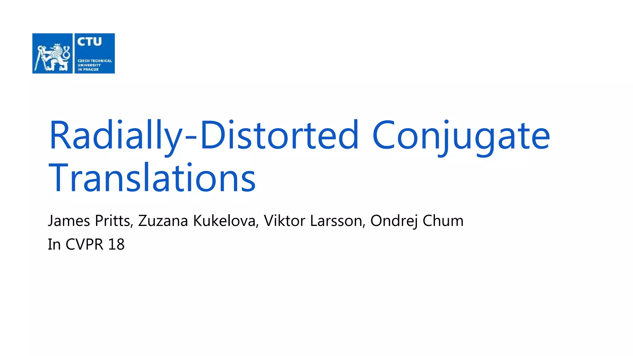
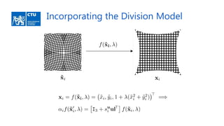
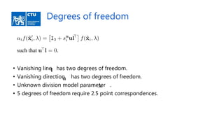
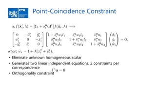
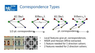
The document discusses a method for joint estimation of lens distortion and rectification, emphasizing the challenges of sampling distortion parameters and the non-convex nature of the problem. It introduces new solvers that utilize the hidden variable trick to reduce unknowns and improve the stability of solutions, while also addressing noise sensitivity in various scenarios. The findings indicate that the proposed solvers are more efficient and accurate compared to traditional methods.


![Polymer [ बहुलक ] Chemistry Notes PDF - Irfanullah Mehar - JJ Sir Chemistry.pdf](https://cdn.slidesharecdn.com/ss_thumbnails/polymerchemistrynotespdf-irfanullahmehar-jjsirchemistry-260210172118-3f9b37f7-thumbnail.jpg?width=640&height=640&fit=bounds)


