This article aims to make the ICMS tax collection forecast considering linear and non-linear models with time series.

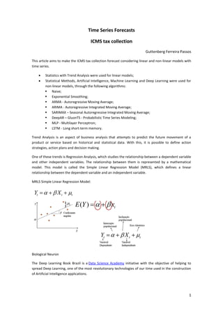
1. 1
Time Series Forecasts
ICMS tax collection
Guttenberg Ferreira Passos
This article aims to make the ICMS tax collection forecast considering linear and non-linear models with
time series.
 Statistics with Trend Analysis were used for linear models;
 Statistical Methods, Artificial Intelligence, Machine Learning and Deep Learning were used for
non-linear models, through the following algorithms:
 Naive;
 Exponential Smoothing;
 ARMA - Autoregressive Moving Average;
 ARIMA - Autoregressive Integrated Moving Average;
 SARIMAX – Seasonal Autoregressive Integrated Moving Average;
 DeepAR – GluonTS - Probabilistic Time Series Modeling;
 MLP - Multilayer Perceptron;
 LSTM - Long short-term memory.
Trend Analysis is an aspect of business analysis that attempts to predict the future movement of a
product or service based on historical and statistical data. With this, it is possible to define action
strategies, action plans and decision making.
One of these trends is Regression Analysis, which studies the relationship between a dependent variable
and other independent variables. The relationship between them is represented by a mathematical
model. This model is called the Simple Linear Regression Model (MRLS), which defines a linear
relationship between the dependent variable and an independent variable.
MRLS Simple Linear Regression Model:
Biological Neuron
The Deep Learning Book Brazil is a Data Science Academy initiative with the objective of helping to
spread Deep Learning, one of the most revolutionary technologies of our time used in the construction
of Artificial Intelligence applications.

2. 2
According to the Deep Learning Book, the biological neuron is a cell, which can be divided into three
sections: the cell body, the dendrites and the axon, each with specific but complementary functions.
Source: Data Science Academy - DSA
Artificial Neuron
An artificial neuron represents the basis of an Artificial Neural Network (ANN), a model of
neuroinformatics oriented to biological neural networks.
Source: Data Science Academy - DSA
The knowledge of an ANN is encoded in the structure of the network, where the connections (synapses)
between the units (neurons) that compose it are highlighted.
Source: Data Science Academy - DSA
In machine learning, Perceptron is a supervised learning algorithm of binary classifiers. A binary classifier
is a function that can decide whether or not an input, represented by a vector of numbers, belongs to
some specific class. It is a type of linear classifier, that is, a classification algorithm that makes its
predictions based on a linear predictor function by combining a set of weights with the vector of
features.

3. 3
Neural Networks
Neural networks are computing systems with interconnected nodes that function like neurons in the
human brain. Using algorithms, they can recognize hidden patterns and correlations in raw data, group
and classify them, and over time continually learn and improve.
Asimov Institute https://www.asimovinstitute.org/neural-network-zoo/ has published a cheat sheet
containing various neural network architectures, we will concentrate on the architectures below
focusing on Perceptron(P), Feed Forward (FF), Recurrent Neural Network (RNN) and Long Short Term
Memory (LSTM):
Source: THE ASIMOV INSTITUTE
Deep learning is one of the foundations of Artificial Intelligence, a type of Machine Learning that trains
computers to perform tasks like humans, which includes speech recognition, image identification and
predictions, learning over time. We can say that it is a Neural Network with several hidden layers:

4. 4
Base Model
Business Problem Definition
ICMS tax collection forecast.
Data set
We use datasets that show ICMS collection. The data has records from the years 2010 to 2015.
Database with 1 dataset with 2 columns, date and ICMS collection, with 96 records:
We noticed that there is a trend of increasing ICMS collection over time.
Exploratory Data Analysis
Let's test the stationarity of the series.
The ACF graph allows the evaluation of the minimum differentiation necessary to obtain a stationary
series (Parameter d for the ARIMA Model):

5. 5
To run the models using Statistical Methods, the data were separated into:
 72 training records and
 24 validation records.
Model 01 - Predictions Simple Linear Regression Method MRLS
Model 11 - Naive Method Forecasts

6. 6
11 – Naive Method
13 - Forecasting – ARIMA LOG (2, 1, 0)
15 – ARMA (1, 0)
15 – ARMA (12, 9)
17 – SARIMAX (0,1,0)(0,1,1,12)
12 – Exponential Smoothing
14 - Forecasting – ARIMA LOG (1, 1, 1)
15 – ARMA (5, 5)
16 - Predict - ARIMA (2, 0, 1)
18 – SARIMAX (0,1,1)(1,1,1,12)

7. 7
Models using:
Inteligência Artificial - IA
22 – LSTM - IA (5 repetitions)
23 – Optimized LSTM - IA
25 – LSTM Bidirectional – IA
RNN01 – MLP Vanilla – IA –
22 – LSTM - IA (20 repetitions)
24 – Stacked LSTM - IA
25 – DeepAR – IA
RNN01 – MLP Window – IA –
Predictions using Artificial Intelligence - AI - Deep Learning

8. 8
RNN02 – LSTM Vanilla IA – Validation
Epoch = 130 - avoid the Overfitting
RNN02 – LSTM Vanilla IA – Validation
Epoch = 200
RNN02 – LSTM Window IA– Validation
RNN02–LSTM Time Steps IA Validation
RNN02 – LSTM Stateful IA – Validation
RNN02 – LSTM Stacked IA – Validation
RNN02 – LSTM Vanilla IA – Test
Epoch = 130 - avoid the Overfitting
RNN02 – LSTM Vanilla IA – Test
Epoch = 200
RNN02 – LSTM Window IA – Test
RNN02 – LSTM Time Steps IA – Test
RNN02 – LSTM Stateful IA – Test
RNN02 – LSTM Stacked IA – Test

9. 9
Model RNN02 – LSTM Vanilla IA – Epoch = 130 – avoid the Overfitting
Model RNN02 – LSTM Vanilla IA – Epoch = 200
Model RNN02 – LSTM Window IA
Model RNN02– LSTM Time Steps

10. 10
Model RNN02– LSTM Stateful
Model RNN02– LSTM Stacked

11. 11
Forecasting using Artificial Intelligence - AI
Model 17 – SARIMAX (0,1,0)(0,1,1,12)
Model 18 – SARIMAX (1,0,1)(1,1,1,12)
Model 22 – LSTM - IA (5 repetitions)
Model 22 – LSTM - IA (20 repetitions)

12. 12
Model 23 – Optimized LSTM - IA
Model 24 – Stacked LSTM - IA
Model 25 – LSTM Bidirectional – IA

13. 13
Model Results:
RSME RSME RSME
Nº Arquitetura Modelo Setup treino validação teste
1 Métodos Estatísticos BASE 11 Método Naive - p/ Mi 0,8054
2 Métodos Estatísticos BASE 11 Método Naive - LOG 0,1551
3 Métodos Estatísticos BASE 11 Método Naive 805471,0878
4 Métodos Estatísticos Forecasting 12 Exponential Smoothing v1 857879,2406
5 Métodos Estatísticos Forecasting 12 Exponential Smoothing v2 750397,7727
6 Métodos Estatísticos ARIMA 13 ARIMA LOG (2, 1, 0) 767631,9506
7 Métodos Estatísticos ARIMA 14 ARIMA LOG (1, 1, 1) 694827,8110
8 Métodos Estatísticos ARMA 15 ARMA (1, 0) 1445179,5400
9 Métodos Estatísticos ARMA 15 ARMA (5, 5) 1101078,9110
10 Métodos Estatísticos ARMA 15 ARMA (12, 9) 706415,3914
11 Métodos Estatísticos ARIMA 16 ARIMA (2, 0, 1) 1099391,396
12 Métodos Estatísticos SARIMAX 17 SARIMAX (0, 1, 0) (0, 1, 1, 12) 332666,2626
13 Métodos Estatísticos SARIMAX 18 SARIMAX (0, 1, 1) (0, 1, 1, 12) 336782,4202
14 IA - Deep Learning LSTM 22 LSTM (5 repetições) 1037107,009
15 IA - Deep Learning LSTM 22 LSTM (20 repetições) 878868,4191
16 IA - Deep Learning LSTM 23 LSTM Otimizado 945778,1667
17 IA - Deep Learning LSTM 24 Stacked LSTM 877490,6632
18 IA - Deep Learning LSTM 25 LSTM Bidirecional 850832,6951
19 IA - Deep Learning DeepAR 26 DeepAR 4874330,639
20 Inteligência Artificial - IA RNA - MLP 1 MLP Vanilla 610423,2630 795393,9775
21 Inteligência Artificial - IA RNA - MLP 2 MLP e Método Window 480295,7828 605733,0842
22 IA - Deep Learning RNN - LSTM 1 LSTM Vanilla - 130 epochs 546148,5770 785606,6766 1417809,7913
23 IA - Deep Learning RNN - LSTM 1 LSTM Vanilla - 200 epochs 496556,0484 586356,0493 950176,2755
24 IA - Deep Learning RNN - LSTM 2 LSTM e Método Window 488946,9051 289236,3698 448340,4022
25 IA - Deep Learning RNN - LSTM 3 LSTM e Time Steps 351787,0114 1184513,5124 1721690,0960
26 IA - Deep Learning RNN - LSTM 4 LSTM e Stateful 444933,0519 549877,8552 911738,8182
27 IA - Deep Learning RNN - LSTM 5 LSTM e Stacked 417403,4958 500538,7458 992971,6186

14. 14
Model Architectures using AI
Model 22 – LSTM - IA (5 repetitions)
Número de repetições = 20
modelo_lstm.add(LSTM(50, activation = 'relu', input_shape = (n_input, n_features)))
modelo_lstm.add(Dropout(0.10))
modelo_lstm.add(Dense(100, activation = 'relu'))
modelo_lstm.add(Dense(100, activation = 'relu'))
modelo_lstm.add(Dense(1))
modelo_lstm.compile(optimizer = 'adam', loss = 'mean_squared_error')
monitor = EarlyStopping(monitor='val_loss', min_delta=1e-3, patience=3, verbose=1, mode='auto')
modelo_lstm.fit_generator(generator, epochs = 200)
Model 23 – Optimized LSTM - IA
Número de repetições = 20
modelo_lstm.add(LSTM(40, activation = 'tanh', return_sequences = True, input_shape = (n_input, n_features)))
modelo_lstm.add(LSTM(40, activation = 'relu'))
modelo_lstm.add(Dense(50, activation = 'relu'))
modelo_lstm.add(Dense(50, activation = 'relu'))
modelo_lstm.add(Dense(1))
adam = optimizers.Adam(lr = 0.001)
modelo_lstm.compile(optimizer = adam, loss = 'mean_squared_error')
monitor = EarlyStopping(monitor='val_loss', min_delta=1e-3, patience=5, verbose=1, mode='auto')
modelo_lstm.fit_generator(generator, epochs = 200)
Model 24 – Stacked LSTM - IA
modelo_lstm.add(LSTM(200, activation = 'relu', return_sequences = True, input_shape = (1, 1)))
modelo_lstm.add(LSTM(100, activation = 'relu', return_sequences = True))
modelo_lstm.add(LSTM(50, activation = 'relu', return_sequences = True))
modelo_lstm.add(LSTM(25, activation = 'relu'))
modelo_lstm.add(Dense(20, activation = 'relu'))
modelo_lstm.add(Dense(10, activation = 'relu'))
modelo_lstm.add(Dense(1))
modelo_lstm.compile(optimizer = 'adam', loss = 'mean_squared_error')
modelo_lstm.fit(X, y, epochs 5000, verbose = 1)
Model 25 – LSTM Bidirectional - IA
Número de repetições = 20
modelo_lstm.add(Bidirectional(LSTM(41, activation = 'relu'), input_shape = (41, 1)))
modelo_lstm.add(Dense(1))
modelo_lstm.compile(optimizer = 'adam', loss = 'mean_squared_error')
modelo_lstm.fit_generator(generator, epochs = 200)
lista_hiperparametros():
n_input = [24]
n_nodes = [100]
n_epochs = [200]
n_batch = [5]
n_diff = [12]
Número de repetições = 20
modelo_lstm.add(Bidirectional(LSTM(100, activation = 'relu'), input_shape = (41, 1)))
modelo_lstm.add(Dense(1))
modelo_lstm.compile(optimizer = 'adam', loss = 'mean_squared_error')
modelo_lstm.fit_generator(generator, epochs = 200)

15. 15
Model Architectures using AI Deep Learning
Model RNN01 – MLP Vanilla – IA
model.add(Dense(8, input_dim = look_back, activation = 'relu'))
model.add(Dense(1))
model.compile(loss = 'mean_squared_error', optimizer = 'adam')
model.fit(trainX, trainY, epochs = 200, batch_size = 2, verbose = 2)
Model RNN01 – MLP Vanilla – IA
model.add(LSTM(4, input_shape = (1, look_back)))
model.add(Dense(1))
model.compile(loss = 'mean_squared_error', optimizer = 'adam')
model.fit(trainX, trainY, epochs = 200, batch_size = 1, verbose = 2)
Model RNN02 – LSTM Vanilla – IA
model.add(LSTM(4, input_shape = (1, look_back)))
model.add(Dense(1))
model.compile(loss = 'mean_squared_error', optimizer = 'adam')
model.fit(trainX, trainY, epochs = 200, batch_size = 1, verbose = 2)
Model RNN02 – LSTM Window – IA
model.add(LSTM(4, input_shape = (1, look_back)))
model.add(Dense(1))
model.compile(loss = 'mean_squared_error', optimizer = 'adam')
model.fit(trainX, trainY, epochs = 200, batch_size = 1, verbose = 2)
Model RNN02 – LSTM Time Steps – IA
model.add(LSTM(4, input_shape = (None, 1)))
model.add(Dense(1))
model.compile(loss = 'mean_squared_error', optimizer = 'adam')
model.fit(trainX, trainY, epochs = 200, batch_size = 1, verbose = 2)
Model RNN02 – LSTM Stateful – IA
model.add(LSTM(4, batch_input_shape = (batch_size, look_back, 1), stateful = True))
model.add(Dense(1))
model.compile(loss = 'mean_squared_error', optimizer = 'adam')
for i in range(200):
model.fit(trainX, trainY, epochs = 1, batch_size = batch_size, verbose = 2, shuffle = False)
model.reset_states()
Model RNN02 – LSTM Stacked – IA
model.add(LSTM(4, batch_input_shape = (batch_size, look_back, 1), stateful = True, return_sequences = True))
model.add(LSTM(4, batch_input_shape = (batch_size, look_back, 1), stateful = True))
model.add(Dense(1))
model.compile(loss = 'mean_squared_error', optimizer = 'adam')
for i in range(200):
model.fit(trainX, trainY, epochs = 1, batch_size = batch_size, verbose = 2, shuffle = False)
model.reset_states()
The models were based on courses from the Data Science Academy DSA and the Community timeline on the portal:
www.datascienceacademy.com.br