okay po i’ll just got off work so i’ll i i’ll will do have the best time and i’ll

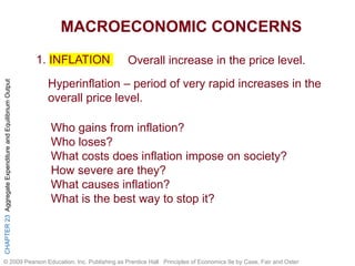
1. CHAPTER
23
Aggregate
Expenditure
and
Equilibrium
Output
© 2009 Pearson Education, Inc. Publishing as Prentice Hall Principles of Economics 9e by Case, Fair and Oster
MACROECONOMIC CONCERNS
1. INFLATION Overall increase in the price level.
Hyperinflation – period of very rapid increases in the
overall price level.
Who gains from inflation?
Who loses?
What costs does inflation impose on society?
How severe are they?
What causes inflation?
What is the best way to stop it?

2. CHAPTER
23
Aggregate
Expenditure
and
Equilibrium
Output
© 2009 Pearson Education, Inc. Publishing as Prentice Hall Principles of Economics 9e by Case, Fair and Oster
2. OUTPUT GROWTH: Short and Long Run
MACROECONOMIC CONCERNS
Economies don’t grow in an even rates at all time.
BUSINESS CYCLE
Aggregate Output – the total quantity of goods and
services produced in an economy in a given period.
Recessions – periods during which aggregate output
declines (2 successive quarters).
Depression – prolonged and deep recession.

3. CHAPTER
23
Aggregate
Expenditure
and
Equilibrium
Output
© 2009 Pearson Education, Inc. Publishing as Prentice Hall Principles of Economics 9e by Case, Fair and Oster
MACROECONOMIC CONCERNS
3. UNEMPLOYMENT The percentage of labor forced that
is unemployed
A key indicator in the health of an economy!
Related to aggregate output
Why do labor markets not clear when other markets
do? (Major economic concern)

4. CHAPTER
23
Aggregate
Expenditure
and
Equilibrium
Output
© 2009 Pearson Education, Inc. Publishing as Prentice Hall Principles of Economics 9e by Case, Fair and Oster
On way the government affects the economy is through its
tax and expenditures decisions (FISCAL POLICY)
The magnitude of TAXES and EXPENDITURES have
major effects in the economy.
Keynes believed that :
Government should cut taxes and / or raise spending
to get the economy out of a slump.
(EXPANSIONARY FISCAL POLICY)
Government should raise taxes and/or cut spending
to bring the economy out of inflation.
(CONTRACTIONARY FISCAL POLICY)

5. CHAPTER
23
Aggregate
Expenditure
and
Equilibrium
Output
© 2009 Pearson Education, Inc. Publishing as Prentice Hall Principles of Economics 9e by Case, Fair and Oster
MONETARY POLICY Through the central bank reserve, the
government can determine the
quantity of money in the economy.
Economists agree that the amount of money in circulation
affects the:
Overall price level
Interest rates
Exchange rates
Unemployment rate
Level of output

6. CHAPTER
23
Aggregate
Expenditure
and
Equilibrium
Output
© 2009 Pearson Education, Inc. Publishing as Prentice Hall Principles of Economics 9e by Case, Fair and Oster
GROWTH POLICIES
Economists believe that the focus of the economy should
be to stimulate aggregate supply.

7. CHAPTER
23
Aggregate
Expenditure
and
Equilibrium
Output
© 2009 Pearson Education, Inc. Publishing as Prentice Hall Principles of Economics 9e by Case, Fair and Oster

8. CHAPTER
23
Aggregate
Expenditure
and
Equilibrium
Output
© 2009 Pearson Education, Inc. Publishing as Prentice Hall Principles of Economics 9e by Case, Fair and Oster
The level of GDP, the overall price level, and the level of
employment—three chief concerns of macroeconomists—
are influenced by events in three broadly defined
“markets”:
Goods-and-services market
Financial (money) market
Labor market

9. CHAPTER
23
Aggregate
Expenditure
and
Equilibrium
Output
© 2009 Pearson Education, Inc. Publishing as Prentice Hall Principles of Economics 9e by Case, Fair and Oster

10. CHAPTER
23
Aggregate
Expenditure
and
Equilibrium
Output
© 2009 Pearson Education, Inc. Publishing as Prentice Hall Principles of Economics 9e by Case, Fair and Oster
Aggregate Expenditure and Equilibrium Output
aggregate output The total quantity of goods and services
produced (or supplied) in an economy in a given period.
aggregate income The total income received by all factors of
production in a given period.
In any given period, there is an exact equality between aggregate
output (production) and aggregate income.
You should be reminded of this fact whenever you encounter the
combined term aggregate output (income) (Y).
aggregate output (income) (Y) A combined term used to remind
you of the exact equality between aggregate output and aggregate
income.

11. CHAPTER
23
Aggregate
Expenditure
and
Equilibrium
Output
© 2009 Pearson Education, Inc. Publishing as Prentice Hall Principles of Economics 9e by Case, Fair and Oster
Income, consumption and Saving (Y, C and S)
(Simple and closed economy)

12. CHAPTER
23
Aggregate
Expenditure
and
Equilibrium
Output
© 2009 Pearson Education, Inc. Publishing as Prentice Hall Principles of Economics 9e by Case, Fair and Oster

13. CHAPTER
23
Aggregate
Expenditure
and
Equilibrium
Output
© 2009 Pearson Education, Inc. Publishing as Prentice Hall Principles of Economics 9e by Case, Fair and Oster
Two types of Spending Behavior
- Spending by Households (consumption)
- Spending by Firms (Investment)
How do households decide how much to consume?
(aggregate consumption depends on the following:
a. Household Income
b. Household wealth
c. Interest Rates
d. Household expectations about the future

14. CHAPTER
23
Aggregate
Expenditure
and
Equilibrium
Output
© 2009 Pearson Education, Inc. Publishing as Prentice Hall Principles of Economics 9e by Case, Fair and Oster
The Keynesian Theory of Consumption
consumption function The relationship between
consumption and income.
A Consumption Function for a
Household
A consumption function for
an individual household
shows the level of
consumption at each level of
household income.
1. Positive slope
2. The intercept of the curve is
above zero

15. CHAPTER
23
Aggregate
Expenditure
and
Equilibrium
Output
© 2009 Pearson Education, Inc. Publishing as Prentice Hall Principles of Economics 9e by Case, Fair and Oster
The Keynesian Theory of Consumption
With a straight line consumption curve, we can use the
following equation to describe the curve:
C = a + bY
An Aggregate Consumption Function
The aggregate consumption function
shows the level of aggregate
consumption at each level of
aggregate income.
The upward slope indicates that
higher levels of income lead to
higher levels of consumption
spending.

16. CHAPTER
23
Aggregate
Expenditure
and
Equilibrium
Output
© 2009 Pearson Education, Inc. Publishing as Prentice Hall Principles of Economics 9e by Case, Fair and Oster
Suppose that the slope is .75, an increase in
income of P100 would increase consumption
by
b∆Y = .75 x 100 = Ᵽ75

17. CHAPTER
23
Aggregate
Expenditure
and
Equilibrium
Output
© 2009 Pearson Education, Inc. Publishing as Prentice Hall Principles of Economics 9e by Case, Fair and Oster
The Keynesian Theory of Consumption
marginal propensity to consume (MPC) That fraction
of a change in income that is consumed or spent.
marginal propensity to consume slope of consumption function
C
Y

 

aggregate saving (S) The part of aggregate income that
is not consumed.
S ≡ Y – C

18. CHAPTER
23
Aggregate
Expenditure
and
Equilibrium
Output
© 2009 Pearson Education, Inc. Publishing as Prentice Hall Principles of Economics 9e by Case, Fair and Oster
The Keynesian Theory of Consumption
identity Something that is always true.
marginal propensity to save (MPS) That fraction of a change in
income that is saved.
MPC + MPS ≡ 1
Because the MPC and the MPS are important concepts, it may help to
review their definitions.
The marginal propensity to consume (MPC) is the fraction of an
increase in income that is consumed (or the fraction of a decrease in
income that comes out of consumption). The marginal propensity to
save (MPS) is the fraction of an increase in income that is saved (or the
fraction of a decrease in income that comes out of saving).

19. CHAPTER
23
Aggregate
Expenditure
and
Equilibrium
Output
© 2009 Pearson Education, Inc. Publishing as Prentice Hall Principles of Economics 9e by Case, Fair and Oster
The Keynesian Theory of Consumption
The Aggregate Consumption
Function Derived from the
Equation C = 100 + .75Y
In this simple consumption function,
consumption is 100 at an income of zero.
As income rises, so does consumption.
For every 100 increase in income,
consumption rises by 75. The slope of
the line is .75.
AGGREGATE
INCOME, Y
(BILLIONS OF
DOLLARS)
AGGREGATE
CONSUMPTION, C
(BILLIONS OF DOLLARS)
0 100
80 160
100 175
200 250
400 400
600 550
800 700
1,000 850

20. CHAPTER
23
Aggregate
Expenditure
and
Equilibrium
Output
© 2009 Pearson Education, Inc. Publishing as Prentice Hall Principles of Economics 9e by Case, Fair and Oster
The Keynesian Theory of Consumption
Deriving the Saving Function from the
Consumption Function
Because S ≡ Y – C, it is easy to derive the
saving function from the consumption
function. A 45° line drawn from the origin can
be used as a convenient tool to compare
consumption and income graphically.
At Y = 200, consumption is 250. The 45° line
shows us that consumption is larger than
income by 50. Thus, S ≡ Y – C = -50.
At Y = 800, consumption is less than income
by 100. Thus, S = 100 when Y = 800.
Y - C = S
AGGREGATE
INCOME
(Billions of Dollars)
AGGREGATE
CONSUMPTION
(Billions of Dollars)
AGGREGATE
SAVING
(Billions of Dollars)
0 100 -100
80 160 -80
100 175 -75
200 250 -50
400 400 0
600 550 50
800 700 100
1,000 850 150

21. CHAPTER
23
Aggregate
Expenditure
and
Equilibrium
Output
© 2009 Pearson Education, Inc. Publishing as Prentice Hall Principles of Economics 9e by Case, Fair and Oster
The Keynesian Theory of Consumption
Other Determinants of Consumption
The assumption that consumption depends only on
income is obviously a simplification. In practice, the
decisions of households on how much to consume in a
given period are also affected by their wealth, by the
interest rate, and by their expectations of the future.
Households with higher wealth are likely to spend more,
other things being equal, than households with less
wealth.

22. CHAPTER
23
Aggregate
Expenditure
and
Equilibrium
Output
© 2009 Pearson Education, Inc. Publishing as Prentice Hall Principles of Economics 9e by Case, Fair and Oster
Planned Investment (I)
The Planned Investment Function
For the time being,
we will assume that
planned investment
is fixed.
It does not change
when income
changes, so its graph
is a horizontal line.

23. CHAPTER
23
Aggregate
Expenditure
and
Equilibrium
Output
© 2009 Pearson Education, Inc. Publishing as Prentice Hall Principles of Economics 9e by Case, Fair and Oster
Planned Investment (I)
planned investment (I) Those additions to capital stock
and inventory that are planned by firms.
actual investment The actual amount of investment that
takes place; it includes items such as unplanned changes
in inventories(UIC).
INPUT INFO: Assume that I is fixed at I = Ᵽ25B and does
not vary with income
(So graphically I is a horizontal line)

24. CHAPTER
23
Aggregate
Expenditure
and
Equilibrium
Output
© 2009 Pearson Education, Inc. Publishing as Prentice Hall Principles of Economics 9e by Case, Fair and Oster
The Determination of Equilibrium Output (Income)
equilibrium Occurs when there is no tendency for change. In the
macroeconomic goods market, equilibrium occurs when planned
aggregate expenditure is equal to aggregate output.
planned aggregate expenditure (AE) The total amount the
economy plans to spend in a given period.
Equal to consumption plus planned investment: AE ≡ C + I.
Y > C + I
aggregate output > planned aggregate expenditure
C + I > Y
planned aggregate expenditure > aggregate output
Equilibrium: Y = AE or Y = C + I
Non-Equilibrium Conditions

25. CHAPTER
23
Aggregate
Expenditure
and
Equilibrium
Output
© 2009 Pearson Education, Inc. Publishing as Prentice Hall Principles of Economics 9e by Case, Fair and Oster
The Determination of Equilibrium Output (Income)
Deriving the Planned Aggregate Expenditure Schedule and Finding Equilibrium
The Figures in Column 2 Are Based on the Equation C = 100 + .75Y.
(1) (2) (3) (4) (5) (6)
Aggregate
Output
(Income) (Y)
Aggregate
Consumption
(C)
Planned
Investment
(I)
Planned
Aggregate
Expenditure
(AE)
C + I
Unplanne
d
Inventory
Change
Y - (C + I)
Equilibrium?
(Y = AE?)
100 175 25 200 - 100 No
200 250 25 275 - 75 No
400 400 25 425 - 25 No
500 475 25 500 0 Yes
600 550 25 575 + 25 No
800 700 25 725 + 75 No
1,000 850 25 875 + 125 No
Equilibrium in the goods market is achieved only when aggregate output
(Y) And planned aggregate expenditure (C + I) are equal, or when
actual and planned investment are equal

26. CHAPTER
23
Aggregate
Expenditure
and
Equilibrium
Output
© 2009 Pearson Education, Inc. Publishing as Prentice Hall Principles of Economics 9e by Case, Fair and Oster
The Determination of Equilibrium Output (Income)
Equilibrium Aggregate Output
Equilibrium occurs when planned
aggregate expenditure and aggregate
output are equal.
Planned aggregate expenditure is the
sum of consumption spending and
planned investment spending.

27. CHAPTER
23
Aggregate
Expenditure
and
Equilibrium
Output
© 2009 Pearson Education, Inc. Publishing as Prentice Hall Principles of Economics 9e by Case, Fair and Oster
Equilibrium computation

28. CHAPTER
23
Aggregate
Expenditure
and
Equilibrium
Output
© 2009 Pearson Education, Inc. Publishing as Prentice Hall Principles of Economics 9e by Case, Fair and Oster
The Determination of Equilibrium Output (Income)
The Saving/Investment Approach to Equilibrium
Because aggregate income must either be saved or spent, by definition,
Y ≡ C + S, which is an identity. The equilibrium condition is Y = C + I, but this
is not an identity because it does not hold when we are out of equilibrium. By
substituting C + S for Y in the equilibrium condition, we can write:
C + S = C + I
Because we can subtract C from both sides of this equation, we are left with:
S = I
Thus, only when planned investment equals saving will there be equilibrium.

29. CHAPTER
23
Aggregate
Expenditure
and
Equilibrium
Output
© 2009 Pearson Education, Inc. Publishing as Prentice Hall Principles of Economics 9e by Case, Fair and Oster
The Determination of Equilibrium Output (Income)
The Saving/Investment Approach to Equilibrium
Aggregate output is equal to
planned aggregate
expenditure only when saving
equals planned investment
(S = I).
Saving and planned
investment are equal at
Y = 500.
The S = I Approach to Equilibrium

30. CHAPTER
23
Aggregate
Expenditure
and
Equilibrium
Output
© 2009 Pearson Education, Inc. Publishing as Prentice Hall Principles of Economics 9e by Case, Fair and Oster
The Determination of Equilibrium Output (Income)
Adjustment to Equilibrium
The adjustment process will continue as long as output
(income) is below planned aggregate expenditure. If firms
react to unplanned inventory reductions by increasing output,
an economy with planned spending greater than output will
adjust to equilibrium, with Y higher than before. If planned
spending is less than output, there will be unplanned increases
in inventories. In this case, firms will respond by reducing
output. As output falls, income falls, consumption falls, and
so on, until equilibrium is restored, with Y lower than
before.

31. CHAPTER
23
Aggregate
Expenditure
and
Equilibrium
Output
© 2009 Pearson Education, Inc. Publishing as Prentice Hall Principles of Economics 9e by Case, Fair and Oster
The Multiplier
multiplier The ratio of the change in the
equilibrium level of output to a change in some
exogenous variable.
exogenous variable A variable that is assumed
not to depend on the state of the economy—that
is, it does not change when the economy
changes.

32. CHAPTER
23
Aggregate
Expenditure
and
Equilibrium
Output
© 2009 Pearson Education, Inc. Publishing as Prentice Hall Principles of Economics 9e by Case, Fair and Oster
The Multiplier
The Multiplier as Seen in the Planned Aggregate Expenditure Diagram
At point A, the economy is in
equilibrium at Y = 500.
When I increases by 25, planned
aggregate expenditure is initially
greater than aggregate output.
As output rises in response,
additional consumption is
generated, pushing equilibrium
output up by a multiple of the
initial increase in I.
The new equilibrium is found at
point B, where Y = 600.
Equilibrium output has increased
by 100 (600 - 500), or four times
the amount of the increase in
planned investment.

33. CHAPTER
23
Aggregate
Expenditure
and
Equilibrium
Output
© 2009 Pearson Education, Inc. Publishing as Prentice Hall Principles of Economics 9e by Case, Fair and Oster
The Multiplier
The Multiplier Equation
MPS
S
Y



MPS
I
Y



Because S must be equal to I for equilibrium to be restored, we can
substitute I for S and solve:
therefore,  
Y I
MPS
 
1
multiplier
MPS

1 , or
multiplier
MPC

-
1
1
The marginal propensity to save may be expressed as: