SlideShare a Scribd company logo
1 of 14
Download to read offline
Technical Note

Roche® LightCycler® 480
Real-Time PCR Run Setup Instructions
for qBiomarker Copy Number PCR Arrays
Preparation
Before the Experiment (Setting up the Run Template):
 Make sure the real-time PCR instrument is working properly. Refer to the manufacturer’s Installation and
Maintenance manual if needed.
 Make sure the correct thermal block cycler (384-well block format for G plate or 96-well for F plate) is in place.
 Turn on the LightCycler 480 instrument; the main switch is located at the back of the instrument. Turn on the
computer linked to the instrument and log on to Window XP.

Creation of PCR Protocol Template
1)
2)
3)
4)

Start LightCycler 480 software 1.5.0 SP4.
Enter Username and Password when the Login dialog box appears and click the
button to proceed with
the login. The Overview window will appear.
Wait for the initiation of the instrument to finish and the two s tatus LEDs on the front of the instrument to
become stable. The left LED should become a steady green while the right LED should be a steady
orange.
In the Overview window (Figure 1), click the New Experiment button on the right-hand side of the window
to launch the Run module.

Figure 1: Overview Window

Page 1 of 14

QIAGEN GmbH  QIAGEN Str. 1  40724 Hilden  Germany  Commercial Register Düsseldorf (HRB 45822)
Managing Directors: Peer M. Schatz, Roland Sackers, Bernd Uder, Dr. Joachim Schorr, Douglas Liu
Technical Note

5)

In the Setup area at the top of the Run Protocol tab (Figure 2), specify the following setup parameters:

Detection Format: SYBR Green I

Block Type: should show the correct block format (384 or 96)

Plate ID: (Optional)

Reaction Volume: 10L for G plate or 25L for F plate

Figure 2: Initial Run Protocol Window

6)

In the Programs section, click the

7)

Click to change the Program Name of the first program to “Heat Activation”. Leave the number of Cycles
at “1” and leave the Analysis Mode as “None”. In the Program Temperature Targets section, enter the
values for the following parameters (See Figure 3):

Target
(C)

Acquisition
Mode

Hold
(hh:mm:ss)

95

None

00:10:00

button twice to add two more program lines.

Ramp
Rate
(C/s)
4.8*

Acquisition
(per C)

Sec
Target
(C)
0

Page 2 of 14

QIAGEN GmbH  QIAGEN Str. 1  40724 Hilden  Germany  Commercial Register Düsseldorf (HRB 45822)
Managing Directors: Peer M. Schatz, Roland Sackers, Bernd Uder, Dr. Joachim Schorr, Douglas Liu

Step
Size
(C)
0

Step
Delay
(cycles)
0
Technical Note

*This is the default ramp rate for 384-well block. The default ramp rate for 96-well block is 4.4˚C/s.

Figure 3: Setup of the 1st Program - Heat Activation

8)

nd

Click to change the Program Name of the 2 program to “PCR Cycling”. Change the number of Cycles
to “45” ** and change the Analysis Mode to “Quantification”. In the Program Temperature Targets
button to add one more temperature target line. Enter the values for the following
section, click the
parameters (Figure 4):

Target
(C)

Acquisition
Mode

Hold
(hh:mm:ss)

95
70

None
Single

00:00:15
00:01:00

Ramp
Rate
(C/s)
1.0
1.0

Acquisition
(per C)

Sec
Target
(C)
0
0

Page 3 of 14

QIAGEN GmbH  QIAGEN Str. 1  40724 Hilden  Germany  Commercial Register Düsseldorf (HRB 45822)
Managing Directors: Peer M. Schatz, Roland Sackers, Bernd Uder, Dr. Joachim Schorr, Douglas Liu

Step
Size
(C)
0
0

Step
Delay
(cycles)
0
0
Technical Note

**Note: The PCR is run for extra five cycles (i.e. 45 cycles) rather than the typical 40 cycles indicated i n the
Handbook as this will allow the use of the Second Derivative Maximum method available with the
LightCycler 480 software for data analysis. See Data Analysis section for further details.
Figure 4: Setup of the 2

9)

nd

Program - PCR Cycling

Click to change the Program Name of the 3 rd program to “Melt Curve”. Leave Cycles at “1” and change
Analysis Mode to “Melting Curves”. In the Temperature Targets section, click the
button once to add
one more temperature target line. Enter the values for the following parameters (Figure 5):

Target
(C)

Acquisition
Mode

Hold
(hh:mm:ss)

60
95

None
Continuous

00:00:15

Ramp
Rate
(C/s)
4.8*
0.03

Acquisition
(per C)

Sec
Target
(C)

Step
Size
(C)

Step
Delay
(cycles)

20

*This is the default ram p rate for 384-well block. The default ramp rate for 96-well block is 4.4˚C/s.

Page 4 of 14

QIAGEN GmbH  QIAGEN Str. 1  40724 Hilden  Germany  Commercial Register Düsseldorf (HRB 45822)
Managing Directors: Peer M. Schatz, Roland Sackers, Bernd Uder, Dr. Joachim Schorr, Douglas Liu
Technical Note

rd

Figure 5: Setup of the 3 Program - Melt Curve

10) Click the down arrow button (
) right next to the Apply Template button on the lower left corner of the
screen; select the Save As Template button (Figure 6) to save the run template under the filename
“CopyNum_PCR_Array_384_LC” if using the 384-well format or “CopyNum_PCR_Array_96_LC” for if
using the 96-well format.

Page 5 of 14

QIAGEN GmbH  QIAGEN Str. 1  40724 Hilden  Germany  Commercial Register Düsseldorf (HRB 45822)
Managing Directors: Peer M. Schatz, Roland Sackers, Bernd Uder, Dr. Joachim Schorr, Douglas Liu
Technical Note

Figure 6: Saving the Run Template File

Page 6 of 14

QIAGEN GmbH  QIAGEN Str. 1  40724 Hilden  Germany  Commercial Register Düsseldorf (HRB 45822)
Managing Directors: Peer M. Schatz, Roland Sackers, Bernd Uder, Dr. Joachim Schorr, Douglas Liu
Technical Note

Performing Real-Time PCR Detection
To load the PCR Array plate and start the run:
1)
2)
3)

After the PCR Array is prepared and centrifuged, bring the plate to the LightCycler 480 instrument to load .
Make sure the correct thermal block (384-well block format for G plate or 96-well for F plate) is in place.
If the instrument is not on, turn it on using the main switch at the back of the instrument. Turn on the
computer linked to the instrument and log on to Window XP.
4) Start LightCycler 480 software.
5) Enter Username and Password when the Login dialog box pops up and click the
button to proceed with
the login. The Overview window will appear.
6) Wait for the two s tatus LEDs on the front of the instrument to become stable. The left LED should become
a steady green while the right LED should be a steady orange.
7) Press the   open/close button on the front of the instrument (located next to the instrument status
LEDs). The plate loading arm will slide out of the right side of the instrument. Place the PCR Array plate
into the frame of the loading arm with the flat edge of the array closest to the instrument and the edge with
a beveled corner pointing away from the instrument.
8) Press the   open/close button again to retract the loading arm . Wait for both of the status LEDs to turn
steady green.
9) In the Overview window, click the New Experiment button on the right-hand side of the screen.
10) In the Run Protocol tab, click the Apply Template button on the lower left corner of the screen. Select
and double click to open the appropriate previously saved “CopyNum_PCR_Array_384_LC” or
“CopyNum_PCR_Array_96_LC” run template file.
11) Press the Start Run button on the lower right corner of the screen to initiate the run. When prompted, save
the file under a new filename after which the run will begin.

Page 7 of 14

QIAGEN GmbH  QIAGEN Str. 1  40724 Hilden  Germany  Commercial Register Düsseldorf (HRB 45822)
Managing Directors: Peer M. Schatz, Roland Sackers, Bernd Uder, Dr. Joachim Schorr, Douglas Liu
Technical Note

Data Analysis
1)

In the Navigator window (Figure 7), find and open the run file to be analyzed.

Figure 7: Opening a completed Run File

Page 8 of 14

QIAGEN GmbH  QIAGEN Str. 1  40724 Hilden  Germany  Commercial Register Düsseldorf (HRB 45822)
Managing Directors: Peer M. Schatz, Roland Sackers, Bernd Uder, Dr. Joachim Schorr, Douglas Liu
Technical Note

2)

For data analysis using the LightCycler 480 we highly recommend the use of the Second Derivative
Maximum analysis method available in this software. This is an algorithm based on the kinetics of a PCR
reaction. This method identifies the crossing point (Cp) of a PCR reaction as the point where the reaction’s
fluorescence reaches the maximum of the second derivative of the amplification curve , which corresponds
to the point where the acceleration of the fluorescence signal is at its maximum. Hence, this crossing point
should always be located in the middle of the log-linear portion of the PCR amplification plot. The
advantage of this analysis m ethod is that it requires little user input and produces consistent results.

3)

Obtaining the Crossing Point (Cp) Cycle values: Once the selected run file is open, click the Analysis
button on the left-hand side of the window. In the Create new analysis list double click to select “Abs
Quant/2nd Derivative Max”. In the “Create new analysis” window that opens, make sure the Analysis
to confirm the selection.
Type is “Abs Quant/2nd Derivative Max” (Figure 8). Click

Figure 8: Setting up the Analysis for the Second Derivative Maximum

Page 9 of 14

QIAGEN GmbH  QIAGEN Str. 1  40724 Hilden  Germany  Commercial Register Düsseldorf (HRB 45822)
Managing Directors: Peer M. Schatz, Roland Sackers, Bernd Uder, Dr. Joachim Schorr, Douglas Liu
Technical Note

4)

The Analysis Window with the amplification curves will appear (Figure 9). To proceed, click the down
) on the lower right corner of the screen to set the analysis to “High Confidence.” Next
arrow button (
click the “Calculate” button to generate Cp values. The calculation may take a few minutes.

Figure 9: Obtaining the Crossing Point (Cp) Cycle Values at the Second Derivative Maximum

5)

Once the Cp values are generated, move the mouse over to the Samples window and click to highlight the
Samples result table. Right click the table and select “Export” button to export the data. A “Save table
data” dialog box will appear (Figure 10). Enter a filename to save the data as a text file. Then click the
button on the right panel to s ave the Second Derivative Maximum Analysis and the Cp values as part of the
run file.

Page 10 of 14

QIAGEN GmbH  QIAGEN Str. 1  40724 Hilden  Germany  Commercial Register Düsseldorf (HRB 45822)
Managing Directors: Peer M. Schatz, Roland Sackers, Bernd Uder, Dr. Joachim Schorr, Douglas Liu
Technical Note

Figure 10: Exporting the Cp Values

6)

To proceed with the melt curve analysis, click the
button located on the right of the Analyses line at the
top of the window. The Create new analysis dialog box will open (Figure 11). Select the “Tm calling” for
the Analysis Type. Then click
to confirm the selection.

Page 11 of 14

QIAGEN GmbH  QIAGEN Str. 1  40724 Hilden  Germany  Commercial Register Düsseldorf (HRB 45822)
Managing Directors: Peer M. Schatz, Roland Sackers, Bernd Uder, Dr. Joachim Schorr, Douglas Liu
Technical Note

Figure 11: Setting up the Melt Curve Analysis

7)

The Analysis window with the raw melt curves will appear (Figure 12). To proceed, click the down arrow
button ( ) on the lower right corner of the screen to set the analysis to “SYBR Green I Format”. Next
click the “Calculate” button. The calculation may take several minutes. Once the melting peaks and Tm
values appear, check the specificity of each assay by ensuring the presence of a single melt peak in each
well. Then click the

button on the right panel to save the melt curve analysis as part of the run file.

Page 12 of 14

QIAGEN GmbH  QIAGEN Str. 1  40724 Hilden  Germany  Commercial Register Düsseldorf (HRB 45822)
Managing Directors: Peer M. Schatz, Roland Sackers, Bernd Uder, Dr. Joachim Schorr, Douglas Liu
Technical Note

Figure 12: Generating Melt Curve Analysis

8)

To save the Melt Peak values: Move the mouse over to the Samples window and click to highlight the
result table. Right click the “Export” button to export the data. A “Save table data” dialog box will appear
(Figure 13). Enter a filename to save the data as a text file.

Page 13 of 14

QIAGEN GmbH  QIAGEN Str. 1  40724 Hilden  Germany  Commercial Register Düsseldorf (HRB 45822)
Managing Directors: Peer M. Schatz, Roland Sackers, Bernd Uder, Dr. Joachim Schorr, Douglas Liu
Technical Note

Figure 13: Exporting the Melt Curve data

Page 14 of 14

QIAGEN GmbH  QIAGEN Str. 1  40724 Hilden  Germany  Commercial Register Düsseldorf (HRB 45822)
Managing Directors: Peer M. Schatz, Roland Sackers, Bernd Uder, Dr. Joachim Schorr, Douglas Liu

More Related Content

Similar to LightCycler 480 Real-Time PCR Run Setup Instructions

Cn eppendorf mastercyclersetup_20120808e
Cn eppendorf mastercyclersetup_20120808eCn eppendorf mastercyclersetup_20120808e
Cn eppendorf mastercyclersetup_20120808eElsa von Licy
 
Cn abi7500 setup_20120808e
Cn abi7500 setup_20120808eCn abi7500 setup_20120808e
Cn abi7500 setup_20120808eElsa von Licy
 
Cn abi7900 ht_setup_201200808e
Cn abi7900 ht_setup_201200808eCn abi7900 ht_setup_201200808e
Cn abi7900 ht_setup_201200808eElsa von Licy
 
Eppendorf mastercyclertechnote
Eppendorf mastercyclertechnoteEppendorf mastercyclertechnote
Eppendorf mastercyclertechnoteElsa von Licy
 
Cn rgq setup_20120808_e
Cn rgq setup_20120808_eCn rgq setup_20120808_e
Cn rgq setup_20120808_eElsa von Licy
 
Mi script mirna_abi7900_technical_note_setup-e
Mi script mirna_abi7900_technical_note_setup-eMi script mirna_abi7900_technical_note_setup-e
Mi script mirna_abi7900_technical_note_setup-eElsa von Licy
 
Cn abi step oneplussetup_20120808e
Cn abi step oneplussetup_20120808eCn abi step oneplussetup_20120808e
Cn abi step oneplussetup_20120808eElsa von Licy
 
Cn mx3000 p_20120808e
Cn mx3000 p_20120808eCn mx3000 p_20120808e
Cn mx3000 p_20120808eElsa von Licy
 
Instrument setuprotorgeneq
Instrument setuprotorgeneqInstrument setuprotorgeneq
Instrument setuprotorgeneqElsa von Licy
 
Mi script mirna_icycler_technical_note_setup-e
Mi script mirna_icycler_technical_note_setup-eMi script mirna_icycler_technical_note_setup-e
Mi script mirna_icycler_technical_note_setup-eElsa von Licy
 
Bio radcfx96 cfx38_setup_instructionse
Bio radcfx96 cfx38_setup_instructionseBio radcfx96 cfx38_setup_instructionse
Bio radcfx96 cfx38_setup_instructionseElsa von Licy
 

Similar to LightCycler 480 Real-Time PCR Run Setup Instructions (20)

Cn eppendorf mastercyclersetup_20120808e
Cn eppendorf mastercyclersetup_20120808eCn eppendorf mastercyclersetup_20120808e
Cn eppendorf mastercyclersetup_20120808e
 
Cn abi7500 setup_20120808e
Cn abi7500 setup_20120808eCn abi7500 setup_20120808e
Cn abi7500 setup_20120808e
 
Cn abi7900 ht_setup_201200808e
Cn abi7900 ht_setup_201200808eCn abi7900 ht_setup_201200808e
Cn abi7900 ht_setup_201200808e
 
Som mx3000 p_setupe
Som mx3000 p_setupeSom mx3000 p_setupe
Som mx3000 p_setupe
 
Eppendorf mastercyclertechnote
Eppendorf mastercyclertechnoteEppendorf mastercyclertechnote
Eppendorf mastercyclertechnote
 
Som abi7500 setup_e
Som abi7500 setup_eSom abi7500 setup_e
Som abi7500 setup_e
 
Som i cycler_setupe
Som i cycler_setupeSom i cycler_setupe
Som i cycler_setupe
 
Som abi7900 setup_e
Som abi7900 setup_eSom abi7900 setup_e
Som abi7900 setup_e
 
Cn rgq setup_20120808_e
Cn rgq setup_20120808_eCn rgq setup_20120808_e
Cn rgq setup_20120808_e
 
Abi7900 ht2.3e
Abi7900 ht2.3eAbi7900 ht2.3e
Abi7900 ht2.3e
 
Abi7900 ht2.1e
Abi7900 ht2.1eAbi7900 ht2.1e
Abi7900 ht2.1e
 
Mi script mirna_abi7900_technical_note_setup-e
Mi script mirna_abi7900_technical_note_setup-eMi script mirna_abi7900_technical_note_setup-e
Mi script mirna_abi7900_technical_note_setup-e
 
Cn abi step oneplussetup_20120808e
Cn abi step oneplussetup_20120808eCn abi step oneplussetup_20120808e
Cn abi step oneplussetup_20120808e
 
Cn mx3000 p_20120808e
Cn mx3000 p_20120808eCn mx3000 p_20120808e
Cn mx3000 p_20120808e
 
Abi75001.3.0 e
Abi75001.3.0 eAbi75001.3.0 e
Abi75001.3.0 e
 
Bio radicycleiq3.1e
Bio radicycleiq3.1eBio radicycleiq3.1e
Bio radicycleiq3.1e
 
Instrument setuprotorgeneq
Instrument setuprotorgeneqInstrument setuprotorgeneq
Instrument setuprotorgeneq
 
Mi script mirna_icycler_technical_note_setup-e
Mi script mirna_icycler_technical_note_setup-eMi script mirna_icycler_technical_note_setup-e
Mi script mirna_icycler_technical_note_setup-e
 
Bio radcfx96 cfx38_setup_instructionse
Bio radcfx96 cfx38_setup_instructionseBio radcfx96 cfx38_setup_instructionse
Bio radcfx96 cfx38_setup_instructionse
 
Som rgq setup_e
Som rgq setup_eSom rgq setup_e
Som rgq setup_e
 

More from Elsa von Licy

Styles of Scientific Reasoning, Scientific Practices and Argument in Science ...
Styles of Scientific Reasoning, Scientific Practices and Argument in Science ...Styles of Scientific Reasoning, Scientific Practices and Argument in Science ...
Styles of Scientific Reasoning, Scientific Practices and Argument in Science ...Elsa von Licy
 
Strategie Decisions Incertitude Actes conference fnege xerfi
Strategie Decisions Incertitude Actes conference fnege xerfiStrategie Decisions Incertitude Actes conference fnege xerfi
Strategie Decisions Incertitude Actes conference fnege xerfiElsa von Licy
 
Neuropsychophysiologie
NeuropsychophysiologieNeuropsychophysiologie
NeuropsychophysiologieElsa von Licy
 
L agressivite en psychanalyse (21 pages 184 ko)
L agressivite en psychanalyse (21 pages   184 ko)L agressivite en psychanalyse (21 pages   184 ko)
L agressivite en psychanalyse (21 pages 184 ko)Elsa von Licy
 
C1 clef pour_la_neuro
C1 clef pour_la_neuroC1 clef pour_la_neuro
C1 clef pour_la_neuroElsa von Licy
 
Vuillez jean philippe_p01
Vuillez jean philippe_p01Vuillez jean philippe_p01
Vuillez jean philippe_p01Elsa von Licy
 
Spr ue3.1 poly cours et exercices
Spr ue3.1   poly cours et exercicesSpr ue3.1   poly cours et exercices
Spr ue3.1 poly cours et exercicesElsa von Licy
 
Plan de cours all l1 l2l3m1m2 p
Plan de cours all l1 l2l3m1m2 pPlan de cours all l1 l2l3m1m2 p
Plan de cours all l1 l2l3m1m2 pElsa von Licy
 
Bioph pharm 1an-viscosit-des_liquides_et_des_solutions
Bioph pharm 1an-viscosit-des_liquides_et_des_solutionsBioph pharm 1an-viscosit-des_liquides_et_des_solutions
Bioph pharm 1an-viscosit-des_liquides_et_des_solutionsElsa von Licy
 
Poly histologie-et-embryologie-medicales
Poly histologie-et-embryologie-medicalesPoly histologie-et-embryologie-medicales
Poly histologie-et-embryologie-medicalesElsa von Licy
 
Methodes travail etudiants
Methodes travail etudiantsMethodes travail etudiants
Methodes travail etudiantsElsa von Licy
 
Atelier.etude.efficace
Atelier.etude.efficaceAtelier.etude.efficace
Atelier.etude.efficaceElsa von Licy
 
There is no_such_thing_as_a_social_science_intro
There is no_such_thing_as_a_social_science_introThere is no_such_thing_as_a_social_science_intro
There is no_such_thing_as_a_social_science_introElsa von Licy
 

More from Elsa von Licy (20)

Styles of Scientific Reasoning, Scientific Practices and Argument in Science ...
Styles of Scientific Reasoning, Scientific Practices and Argument in Science ...Styles of Scientific Reasoning, Scientific Practices and Argument in Science ...
Styles of Scientific Reasoning, Scientific Practices and Argument in Science ...
 
Strategie Decisions Incertitude Actes conference fnege xerfi
Strategie Decisions Incertitude Actes conference fnege xerfiStrategie Decisions Incertitude Actes conference fnege xerfi
Strategie Decisions Incertitude Actes conference fnege xerfi
 
Rainville pierre
Rainville pierreRainville pierre
Rainville pierre
 
Neuropsychophysiologie
NeuropsychophysiologieNeuropsychophysiologie
Neuropsychophysiologie
 
L agressivite en psychanalyse (21 pages 184 ko)
L agressivite en psychanalyse (21 pages   184 ko)L agressivite en psychanalyse (21 pages   184 ko)
L agressivite en psychanalyse (21 pages 184 ko)
 
C1 clef pour_la_neuro
C1 clef pour_la_neuroC1 clef pour_la_neuro
C1 clef pour_la_neuro
 
Hemostase polycop
Hemostase polycopHemostase polycop
Hemostase polycop
 
Antiphilos
AntiphilosAntiphilos
Antiphilos
 
Vuillez jean philippe_p01
Vuillez jean philippe_p01Vuillez jean philippe_p01
Vuillez jean philippe_p01
 
Spr ue3.1 poly cours et exercices
Spr ue3.1   poly cours et exercicesSpr ue3.1   poly cours et exercices
Spr ue3.1 poly cours et exercices
 
Plan de cours all l1 l2l3m1m2 p
Plan de cours all l1 l2l3m1m2 pPlan de cours all l1 l2l3m1m2 p
Plan de cours all l1 l2l3m1m2 p
 
M2 bmc2007 cours01
M2 bmc2007 cours01M2 bmc2007 cours01
M2 bmc2007 cours01
 
Feuilletage
FeuilletageFeuilletage
Feuilletage
 
Chapitre 1
Chapitre 1Chapitre 1
Chapitre 1
 
Biophy
BiophyBiophy
Biophy
 
Bioph pharm 1an-viscosit-des_liquides_et_des_solutions
Bioph pharm 1an-viscosit-des_liquides_et_des_solutionsBioph pharm 1an-viscosit-des_liquides_et_des_solutions
Bioph pharm 1an-viscosit-des_liquides_et_des_solutions
 
Poly histologie-et-embryologie-medicales
Poly histologie-et-embryologie-medicalesPoly histologie-et-embryologie-medicales
Poly histologie-et-embryologie-medicales
 
Methodes travail etudiants
Methodes travail etudiantsMethodes travail etudiants
Methodes travail etudiants
 
Atelier.etude.efficace
Atelier.etude.efficaceAtelier.etude.efficace
Atelier.etude.efficace
 
There is no_such_thing_as_a_social_science_intro
There is no_such_thing_as_a_social_science_introThere is no_such_thing_as_a_social_science_intro
There is no_such_thing_as_a_social_science_intro
 

LightCycler 480 Real-Time PCR Run Setup Instructions

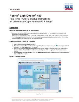
  • 1. Technical Note Roche® LightCycler® 480 Real-Time PCR Run Setup Instructions for qBiomarker Copy Number PCR Arrays Preparation Before the Experiment (Setting up the Run Template):  Make sure the real-time PCR instrument is working properly. Refer to the manufacturer’s Installation and Maintenance manual if needed.  Make sure the correct thermal block cycler (384-well block format for G plate or 96-well for F plate) is in place.  Turn on the LightCycler 480 instrument; the main switch is located at the back of the instrument. Turn on the computer linked to the instrument and log on to Window XP. Creation of PCR Protocol Template 1) 2) 3) 4) Start LightCycler 480 software 1.5.0 SP4. Enter Username and Password when the Login dialog box appears and click the button to proceed with the login. The Overview window will appear. Wait for the initiation of the instrument to finish and the two s tatus LEDs on the front of the instrument to become stable. The left LED should become a steady green while the right LED should be a steady orange. In the Overview window (Figure 1), click the New Experiment button on the right-hand side of the window to launch the Run module. Figure 1: Overview Window Page 1 of 14 QIAGEN GmbH  QIAGEN Str. 1  40724 Hilden  Germany  Commercial Register Düsseldorf (HRB 45822) Managing Directors: Peer M. Schatz, Roland Sackers, Bernd Uder, Dr. Joachim Schorr, Douglas Liu
  • 2. Technical Note 5) In the Setup area at the top of the Run Protocol tab (Figure 2), specify the following setup parameters:  Detection Format: SYBR Green I  Block Type: should show the correct block format (384 or 96)  Plate ID: (Optional)  Reaction Volume: 10L for G plate or 25L for F plate Figure 2: Initial Run Protocol Window 6) In the Programs section, click the 7) Click to change the Program Name of the first program to “Heat Activation”. Leave the number of Cycles at “1” and leave the Analysis Mode as “None”. In the Program Temperature Targets section, enter the values for the following parameters (See Figure 3): Target (C) Acquisition Mode Hold (hh:mm:ss) 95 None 00:10:00 button twice to add two more program lines. Ramp Rate (C/s) 4.8* Acquisition (per C) Sec Target (C) 0 Page 2 of 14 QIAGEN GmbH  QIAGEN Str. 1  40724 Hilden  Germany  Commercial Register Düsseldorf (HRB 45822) Managing Directors: Peer M. Schatz, Roland Sackers, Bernd Uder, Dr. Joachim Schorr, Douglas Liu Step Size (C) 0 Step Delay (cycles) 0
  • 3. Technical Note *This is the default ramp rate for 384-well block. The default ramp rate for 96-well block is 4.4˚C/s. Figure 3: Setup of the 1st Program - Heat Activation 8) nd Click to change the Program Name of the 2 program to “PCR Cycling”. Change the number of Cycles to “45” ** and change the Analysis Mode to “Quantification”. In the Program Temperature Targets button to add one more temperature target line. Enter the values for the following section, click the parameters (Figure 4): Target (C) Acquisition Mode Hold (hh:mm:ss) 95 70 None Single 00:00:15 00:01:00 Ramp Rate (C/s) 1.0 1.0 Acquisition (per C) Sec Target (C) 0 0 Page 3 of 14 QIAGEN GmbH  QIAGEN Str. 1  40724 Hilden  Germany  Commercial Register Düsseldorf (HRB 45822) Managing Directors: Peer M. Schatz, Roland Sackers, Bernd Uder, Dr. Joachim Schorr, Douglas Liu Step Size (C) 0 0 Step Delay (cycles) 0 0
  • 4. Technical Note **Note: The PCR is run for extra five cycles (i.e. 45 cycles) rather than the typical 40 cycles indicated i n the Handbook as this will allow the use of the Second Derivative Maximum method available with the LightCycler 480 software for data analysis. See Data Analysis section for further details. Figure 4: Setup of the 2 9) nd Program - PCR Cycling Click to change the Program Name of the 3 rd program to “Melt Curve”. Leave Cycles at “1” and change Analysis Mode to “Melting Curves”. In the Temperature Targets section, click the button once to add one more temperature target line. Enter the values for the following parameters (Figure 5): Target (C) Acquisition Mode Hold (hh:mm:ss) 60 95 None Continuous 00:00:15 Ramp Rate (C/s) 4.8* 0.03 Acquisition (per C) Sec Target (C) Step Size (C) Step Delay (cycles) 20 *This is the default ram p rate for 384-well block. The default ramp rate for 96-well block is 4.4˚C/s. Page 4 of 14 QIAGEN GmbH  QIAGEN Str. 1  40724 Hilden  Germany  Commercial Register Düsseldorf (HRB 45822) Managing Directors: Peer M. Schatz, Roland Sackers, Bernd Uder, Dr. Joachim Schorr, Douglas Liu
  • 5. Technical Note rd Figure 5: Setup of the 3 Program - Melt Curve 10) Click the down arrow button ( ) right next to the Apply Template button on the lower left corner of the screen; select the Save As Template button (Figure 6) to save the run template under the filename “CopyNum_PCR_Array_384_LC” if using the 384-well format or “CopyNum_PCR_Array_96_LC” for if using the 96-well format. Page 5 of 14 QIAGEN GmbH  QIAGEN Str. 1  40724 Hilden  Germany  Commercial Register Düsseldorf (HRB 45822) Managing Directors: Peer M. Schatz, Roland Sackers, Bernd Uder, Dr. Joachim Schorr, Douglas Liu
  • 6. Technical Note Figure 6: Saving the Run Template File Page 6 of 14 QIAGEN GmbH  QIAGEN Str. 1  40724 Hilden  Germany  Commercial Register Düsseldorf (HRB 45822) Managing Directors: Peer M. Schatz, Roland Sackers, Bernd Uder, Dr. Joachim Schorr, Douglas Liu
  • 7. Technical Note Performing Real-Time PCR Detection To load the PCR Array plate and start the run: 1) 2) 3) After the PCR Array is prepared and centrifuged, bring the plate to the LightCycler 480 instrument to load . Make sure the correct thermal block (384-well block format for G plate or 96-well for F plate) is in place. If the instrument is not on, turn it on using the main switch at the back of the instrument. Turn on the computer linked to the instrument and log on to Window XP. 4) Start LightCycler 480 software. 5) Enter Username and Password when the Login dialog box pops up and click the button to proceed with the login. The Overview window will appear. 6) Wait for the two s tatus LEDs on the front of the instrument to become stable. The left LED should become a steady green while the right LED should be a steady orange. 7) Press the   open/close button on the front of the instrument (located next to the instrument status LEDs). The plate loading arm will slide out of the right side of the instrument. Place the PCR Array plate into the frame of the loading arm with the flat edge of the array closest to the instrument and the edge with a beveled corner pointing away from the instrument. 8) Press the   open/close button again to retract the loading arm . Wait for both of the status LEDs to turn steady green. 9) In the Overview window, click the New Experiment button on the right-hand side of the screen. 10) In the Run Protocol tab, click the Apply Template button on the lower left corner of the screen. Select and double click to open the appropriate previously saved “CopyNum_PCR_Array_384_LC” or “CopyNum_PCR_Array_96_LC” run template file. 11) Press the Start Run button on the lower right corner of the screen to initiate the run. When prompted, save the file under a new filename after which the run will begin. Page 7 of 14 QIAGEN GmbH  QIAGEN Str. 1  40724 Hilden  Germany  Commercial Register Düsseldorf (HRB 45822) Managing Directors: Peer M. Schatz, Roland Sackers, Bernd Uder, Dr. Joachim Schorr, Douglas Liu
  • 8. Technical Note Data Analysis 1) In the Navigator window (Figure 7), find and open the run file to be analyzed. Figure 7: Opening a completed Run File Page 8 of 14 QIAGEN GmbH  QIAGEN Str. 1  40724 Hilden  Germany  Commercial Register Düsseldorf (HRB 45822) Managing Directors: Peer M. Schatz, Roland Sackers, Bernd Uder, Dr. Joachim Schorr, Douglas Liu
  • 9. Technical Note 2) For data analysis using the LightCycler 480 we highly recommend the use of the Second Derivative Maximum analysis method available in this software. This is an algorithm based on the kinetics of a PCR reaction. This method identifies the crossing point (Cp) of a PCR reaction as the point where the reaction’s fluorescence reaches the maximum of the second derivative of the amplification curve , which corresponds to the point where the acceleration of the fluorescence signal is at its maximum. Hence, this crossing point should always be located in the middle of the log-linear portion of the PCR amplification plot. The advantage of this analysis m ethod is that it requires little user input and produces consistent results. 3) Obtaining the Crossing Point (Cp) Cycle values: Once the selected run file is open, click the Analysis button on the left-hand side of the window. In the Create new analysis list double click to select “Abs Quant/2nd Derivative Max”. In the “Create new analysis” window that opens, make sure the Analysis to confirm the selection. Type is “Abs Quant/2nd Derivative Max” (Figure 8). Click Figure 8: Setting up the Analysis for the Second Derivative Maximum Page 9 of 14 QIAGEN GmbH  QIAGEN Str. 1  40724 Hilden  Germany  Commercial Register Düsseldorf (HRB 45822) Managing Directors: Peer M. Schatz, Roland Sackers, Bernd Uder, Dr. Joachim Schorr, Douglas Liu
  • 10. Technical Note 4) The Analysis Window with the amplification curves will appear (Figure 9). To proceed, click the down ) on the lower right corner of the screen to set the analysis to “High Confidence.” Next arrow button ( click the “Calculate” button to generate Cp values. The calculation may take a few minutes. Figure 9: Obtaining the Crossing Point (Cp) Cycle Values at the Second Derivative Maximum 5) Once the Cp values are generated, move the mouse over to the Samples window and click to highlight the Samples result table. Right click the table and select “Export” button to export the data. A “Save table data” dialog box will appear (Figure 10). Enter a filename to save the data as a text file. Then click the button on the right panel to s ave the Second Derivative Maximum Analysis and the Cp values as part of the run file. Page 10 of 14 QIAGEN GmbH  QIAGEN Str. 1  40724 Hilden  Germany  Commercial Register Düsseldorf (HRB 45822) Managing Directors: Peer M. Schatz, Roland Sackers, Bernd Uder, Dr. Joachim Schorr, Douglas Liu
  • 11. Technical Note Figure 10: Exporting the Cp Values 6) To proceed with the melt curve analysis, click the button located on the right of the Analyses line at the top of the window. The Create new analysis dialog box will open (Figure 11). Select the “Tm calling” for the Analysis Type. Then click to confirm the selection. Page 11 of 14 QIAGEN GmbH  QIAGEN Str. 1  40724 Hilden  Germany  Commercial Register Düsseldorf (HRB 45822) Managing Directors: Peer M. Schatz, Roland Sackers, Bernd Uder, Dr. Joachim Schorr, Douglas Liu
  • 12. Technical Note Figure 11: Setting up the Melt Curve Analysis 7) The Analysis window with the raw melt curves will appear (Figure 12). To proceed, click the down arrow button ( ) on the lower right corner of the screen to set the analysis to “SYBR Green I Format”. Next click the “Calculate” button. The calculation may take several minutes. Once the melting peaks and Tm values appear, check the specificity of each assay by ensuring the presence of a single melt peak in each well. Then click the button on the right panel to save the melt curve analysis as part of the run file. Page 12 of 14 QIAGEN GmbH  QIAGEN Str. 1  40724 Hilden  Germany  Commercial Register Düsseldorf (HRB 45822) Managing Directors: Peer M. Schatz, Roland Sackers, Bernd Uder, Dr. Joachim Schorr, Douglas Liu
  • 13. Technical Note Figure 12: Generating Melt Curve Analysis 8) To save the Melt Peak values: Move the mouse over to the Samples window and click to highlight the result table. Right click the “Export” button to export the data. A “Save table data” dialog box will appear (Figure 13). Enter a filename to save the data as a text file. Page 13 of 14 QIAGEN GmbH  QIAGEN Str. 1  40724 Hilden  Germany  Commercial Register Düsseldorf (HRB 45822) Managing Directors: Peer M. Schatz, Roland Sackers, Bernd Uder, Dr. Joachim Schorr, Douglas Liu
  • 14. Technical Note Figure 13: Exporting the Melt Curve data Page 14 of 14 QIAGEN GmbH  QIAGEN Str. 1  40724 Hilden  Germany  Commercial Register Düsseldorf (HRB 45822) Managing Directors: Peer M. Schatz, Roland Sackers, Bernd Uder, Dr. Joachim Schorr, Douglas Liu