This document describes a stateless model that was created using the StateAMS tool to model an aerospace defense customer's system. The model approximates a rational integral using the Riemann summation method by dividing the interval into 20 equal sub-intervals. The StateAMS tool generated a template for the stateless model with ports for input, output, and feedback voltages. The template defines the continuous variables and static parameters to calculate the output current as the sum of 20 rectangular areas approximating the integral.

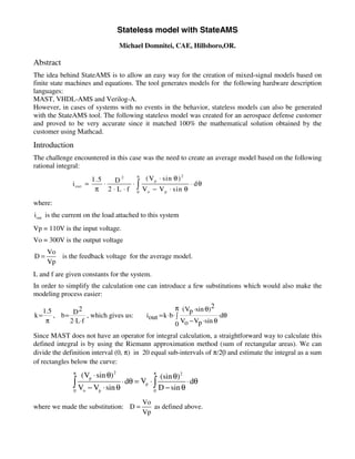
1. Stateless model with StateAMS
Michael Domnitei, CAE, Hillsboro,OR.
Abstract
The idea behind StateAMS is to allow an easy way for the creation of mixed-signal models based on
finite state machines and equations. The tool generates models for the following hardware description
languages:
MAST, VHDL-AMS and Verilog-A.
However, in cases of systems with no events in the behavior, stateless models can also be generated
with the StateAMS tool. The following stateless model was created for an aerospace defense customer
and proved to be very accurate since it matched 100% the mathematical solution obtained by the
customer using Mathcad.
Introduction
The challenge encountered in this case was the need to create an average model based on the following
rational integral:
1.5 D
2 π
(V p ⋅ sin θ ) 2
π 2 ⋅ L ⋅ f ∫ V o − V p ⋅ sin θ
i out = ⋅ ⋅ ⋅ dθ
0
where:
i out is the current on the load attached to this system
Vp = 110V is the input voltage.
Vo = 300V is the output voltage
Vo
D= is the feedback voltage for the average model.
Vp
L and f are given constants for the system.
In order to simplify the calculation one can introduce a few substitutions which would also make the
modeling process easier:
π (Vp ⋅sin θ)2
k=
1.5
, b=
D 2 , which gives us: iout = k ⋅ b ⋅ ∫ ⋅ dθ
π 2 ⋅ L ⋅f 0 Vo − Vp ⋅sin θ
Since MAST does not have an operator for integral calculation, a straightforward way to calculate this
defined integral is by using the Riemann approximation method (sum of rectangular areas). We can
divide the definition interval (0, π) in 20 equal sub-intervals of π/20 DQG HVWLPDWH WKH LQWHJUDO DV D VXP
of rectangles below the curve:
π
(Vp ⋅ sin θ) 2 π
(sin θ)2
∫ Vo − Vp ⋅ sin θ ⋅ dθ = Vp ⋅ ∫ D − sin θ ⋅ dθ
0 0
Vo
where we made the substitution: D = as defined above.
Vp

2. Modeling process
Using the sum of rectangular areas, the rational integral can be approximated as follows:
i
π (sin π)2
(sin θ) 2 π 20 20
∫ D − sin θ ⋅ dθ = 20 i∑1 = i
π
0 D − sin π
20
At this point in time we can see that the original problem has become:
i
(sin π)2
π 20 20
iout = k ⋅b⋅ ∑ π
20 i =1 i
D − sin π
20
The system requirements point to a model topology with 3 conservative ports:
- input voltage (Vp)
- output voltage (Vo)
- feedback (duty) voltage
Since b and D depend on the input and output voltages, they will be defined as continuous variable.
Our main continuous variable is i out which is the sum of the 20 components (i1,i2,…i20).
The static variables of our model are:
- n (the number of sub-intervals)
- π (defined as 3.14)
- L, f, and k are constants which have been introduced in the beginning.
There are no states defined or specified for the behavioral description of this model. However, with all
the information provided, we can create a stateless model using StateAMS tool.
Following is the template auto-generated by the StateAMS tool:
# Created with StateAMS 1.5.
element template integral in out vduty = pi, n, l, f
electrical in, out, vduty
number pi=3.14159, n=20, l=18e-6, f=50e3
{
val v vp, vo, duty
val i iout
val nu i1, i2, i3, i4, i5, i6, i7, i8, i9, i10, a, b, i11, i12, i13, i14, i15,
i16, i17, i18, i19, i20
number k
parameters {
k=1.5/pi
}
values {
vp=v(in)
vo=v(out)
duty=v(vduty)
a=vo/(vp+1p)
b=0.5*duty**2/l/f
i1=sin(pi/n)**2/(a-sin(pi/n))
i2=sin(2*pi/n)**2/(a-sin(2*pi/n))
i3=sin(3*pi/n)**2/(a-sin(3*pi/n))
i4=sin(4*pi/n)**2/(a-sin(4*pi/n))
i5=sin(5*pi/n)**2/(a-sin(5*pi/n))
i6=sin(6*pi/n)**2/(a-sin(6*pi/n))
i7=sin(7*pi/n)**2/(a-sin(7*pi/n))
i8=sin(8*pi/n)**2/(a-sin(8*pi/n))
i9=sin(9*pi/n)**2/(a-sin(9*pi/n))
i10=sin(10*pi/n)**2/(a-sin(10*pi/n))

3. i11=sin(11*pi/n)**2/(a-sin(11*pi/n))
i12=sin(12*pi/n)**2/(a-sin(12*pi/n))
i13=sin(13*pi/n)**2/(a-sin(13*pi/n))
i14=sin(14*pi/n)**2/(a-sin(14*pi/n))
i15=sin(15*pi/n)**2/(a-sin(15*pi/n))
i16=sin(16*pi/n)**2/(a-sin(16*pi/n))
i17=sin(17*pi/n)**2/(a-sin(17*pi/n))
i18=sin(18*pi/n)**2/(a-sin(18*pi/n))
i19=sin(19*pi/n)**2/(a-sin(19*pi/n))
i20=sin(20*pi/n)**2/(a-sin(20*pi/n))
iout=pi*vp*b*k*(i1+i2+i3+i4+i5+i6+i7+i8+i9+i10+i11+i12+i13+i14+i15+i16+i17+i18+i19
+i20)/n
}
equations {
i(out)+=iout
}
}