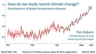
How do we study recent climate change? Development of global temperature datasets
•
0 likes•19 views

Presented by Tim Osborn at the Royal Meteorological Society's meeting on the History of climate science ideas & their application, March 2022

Recommended
Recommended
More Related Content
Similar to How do we study recent climate change? Development of global temperature datasets
Similar to How do we study recent climate change? Development of global temperature datasets (20)
More from Tim Osborn
More from Tim Osborn (6)
Recently uploaded
Recently uploaded (20)
How do we study recent climate change? Development of global temperature datasets
- 1. How do we study recent climate change? Development of global temperature datasets Royal Met. Soc. History of climate science ideas & their application March 2022 Tim Osborn Climatic Research Unit University of East Anglia
- 2. From Ed Hawkins (https://www.climate-lab-book.ac.uk/2015/what-have-global-temperatures-ever-done-for-us) Based on Sutton, Suckling & Hawkins (2015) Phil. Trans. A
- 3. Why global temperature? If we want to know about local climate on short timescales, then unforced variability matters most • Especially from natural variability in atmospheric circulation If we want to know about forced climate change, it becomes clearer at large spatial scales • Global patterns and global means But forced climate change becomes relevant even for local scales when we want to understand or predict longer timescales • Trends or changes on multi-decadal or longer timescales
- 4. Milestones towards global temperature series Networks, compilations & standardisation of observations • Land observations. Examples (not exhaustive): • 1781 onwards: Meteorological Society of Mannheim, network with standards • 1868 onwards: recommendations for Stevenson screens • 1873: First international meteorology meeting Leipzig, predecessor to WMO • 1900: Data sharing system for all continents (except Antarctica) • 1927: World Weather Records • 1948: Monthly Climatic Data for the World • Marine observations. Examples (not exhaustive): • ~1853: Semi-standardised naval logs (Maury, 1849; Quetelet, 1854) • 1966: Digital archives of ship observations begin to be compiled • 1981-1985: Preparation of COADS (Comprehensive Ocea-Atmosphere Data Set) by US, evolved into ICOADS (International COADS)
- 5. Milestones towards global temperature series Analyses and published series (not exhaustive): • Köppen (from 1873) • Already considering issues of quality, homogeneity, uneven data coverage • Callendar (1938) • Neighbour comparisons and metadata used to discard inhomogeneous series • Revisited & improved 1961 (& other series by Willett, 1950; Mitchell, 1963) • Budyko (1963) • Based on hand-drawn maps: less objective but could bring in ocean data • Hansen et al. (NASA GISS) & Jones et al. (Climatic Research Unit, CRU) early 1980s • Gridded datasets of temperature anomalies • 1986 CRU undertook first homogenisation effort on a global-scale network • Jones, Wigley & Wright (1986) – forerunner to HadCRUT • First global land & ocean homogenized global temperature series 1861-1984
- 7. Why use temperature anomalies?
- 12. Why use temperature anomalies? Separation into time-invariant fields (geographical and annual cycle) and time-varying anomalies has many benefits • Simplifies spatial structures in the data which facilitates interpolation • Reduces impact from changes in data coverage (e.g. reduces biases from a changing observation network) • Reduces impact of differences in measurement practice, how to calculate daily means, instruments and exposures, microclimates • These latter aspects can give materially different mean levels, but have much less effect on changes over time* • *provided they don’t change over time – then we need to deal with changing biases over time (inhomogeneity)
- 13. Why use temperature anomalies? When were the benefits of using anomalies first realised? • Unsure! Callendar (1938) already uses them without justifying them. Just seems an obvious way to deal with issues! Even before 1900 (e.g. Dove in the 1850s used anomalies to reduce effect of elevation) There are disadvantages of anomalies too: • Series for which we don’t know the reference period temperature for that station (location, exposure & instrument) can’t necessarily be used • Berkeley Earth (Rohde et al. 2013) introduced a similar approach (separation into deviations from expected values) but which doesn’t use a fixed reference period • This opens up many possibilities – including new ways of dealing with inhomogeneities: just split a series into sub-series that are individually homogeneous
- 14. What about those inhomogeneities? Example: “exposure bias” due to the change from older types of exposure to Stevenson screens • Analyses from Emily Wallis (Climatic Research Unit, UEA)
- 15. Stevenson-type Open Wall Intermediate Closed Unknown Emily Wallis (CRU, UEA) Estimated exposure types 1850-1930
- 16. Exposure bias example: “open” screens Stevenson screen minus “open” screen Stevenson screens tends to read cooler Tmax and warmer Tmin than “open” screens There is a clear seasonal cycle to the bias (except in Tmin) The bias is greatest in Tmax and DTR , but can lead to a monthly bias in Tmean of up to 1.1°C. Parallel Measurement Studies Difference between the thermometer reading in the Stevenson screen and the “open” screen Data sources: Adelaide Observatory Yearbooks; Detwiller, 1978; Ellis, 1891; Gaster, 1882; Gill, 1882; Greenwich Observatory Yearbooks; Margary, 1924; Mawley, 1897; SDATS/AEMET (Brunet, pers. comms) *Monthly data for the Southern Hemisphere studies has been shifted 6 months so the seasons align * Emily Wallis (CRU, UEA)
- 17. How many observations are needed? Surprisingly small number of stations needed to estimate global mean, if they are well distributed, long and reliable Various authors in the 1980s and 1990s tried to estimate how many (e.g. Hansen; Livezey & Chen; Jones & Briffa; Madden) Depends on timescale and on the dominance of any forced climate change (e.g. as few as 40 stations for seasonal, 20 annual, 10 decadal) And we want many more than the minimum number, so overlapping information can help with addressing issues with imperfect data!
- 18. Updated from Jones, Osborn, Briffa (1997) J. Geophys. Res.; based on CRUTEM4 data
- 19. Updated from Jones, Osborn, Briffa (1997) J. Geophys. Res.; based on CRUTEM4 data
- 20. Updated from Jones, Osborn, Briffa (1997) J. Geophys. Res.; based on CRUTEM4 data
- 21. Updated from Jones, Osborn, Briffa (1997) J. Geophys. Res.; based on CRUTEM4 data
- 22. Updated from Jones, Osborn, Briffa (1997) J. Geophys. Res.; based on CRUTEM4 data
- 23. Updated from Jones, Osborn, Briffa (1997) J. Geophys. Res.; based on CRUTEM4 data
- 24. Updated from Jones, Osborn, Briffa (1997) J. Geophys. Res.; based on CRUTEM4 data
- 25. Updated from Jones, Osborn, Briffa (1997) J. Geophys. Res.; based on CRUTEM4 data
- 26. What about the oceans? Sea surface temperature (SST) observations have usually been preferred • SST varies more slowly and with smaller diurnal cycle, so can estimate monthly means from a small number of observations • Day time marine air temperature measurements have traditionally been excluded (due to heating of ship superstructures causing a warm bias that varies over time) • Night marine air temperature (NMAT) increasingly used in recent years: NMAT may have issues, but they tend to be different to the SST biases so there is value in utilising both types of data
- 27. Before 1850, most observations are MAT not SST, and most MAT are daytime GloSAT project (led by Liz Kent at National Oceanography Centre) is grasping this nettle so we can extend back pre-1850 MAT coverage SST coverage % of Marine Air Temperatures taken during the day Figure from Tom Cropper, National Oceanography Centre
- 28. What have we learned from global temperature datasets?
- 29. Derived from Morice et al. (2021) J. Geophys. Res. How much has the globe warmed? (Relevant to policy goals e.g. Paris Agreement)
- 30. Derived from Morice et al. (2021) J. Geophys. Res. How much has the globe warmed? (Relevant to policy goals e.g. Paris Agreement)
- 31. Degrees Celsius difference from the 1961-1990 average HadCRUT5 Analysis annual-mean temperature anomaly maps (https://crudata.uea.ac.uk/~timo/diag/tempdiag.htm)
- 32. Updated from Osborn et al. (2007) Weather Now using HadCRUT5, HadSST4 and CRUTEM5 We understand the mechanisms that determine the warming patterns at the largest scales, including Arctic amplification, land–ocean warming contrast and suppression of warming in the sub-polar oceans Arctic amplification Land Ocean Sub-polar oceans
- 33. Recent developments: HadCRUT5 (improved consideration of SST biases) (improved consideration of incomplete coverage biases) (previous version)
- 35. Slower warming in the early 21st century IPCC’s 2013 assessment was that the difference between observed warming and climate model simulations during this period could be explained as a combination of: (a) unforced variability; (b) errors in the forcing used in models; (c) model errors. Observational dataset error should have been considered too!
- 36. Key points • Recent developments demonstrate that there is more to do than routine updating! • Even though we have a robust record, research underway into extending to earlier periods and reducing biases/inhomogeneities – Rare for improvements to dramatically alter the global-scale picture • Milestones – Standardised measurements – Data sharing and building of data compilations – Dealing with issues: using anomalies, addressing biases, incomplete and uneven spatial coverage
- 37. Spare slides
- 38. Why global temperature? Some definitions: Unforced climate variability • From the inherent variability in the atmosphere and oceans (& ice, land surface) Forced climate change • Caused by forcing (radiative forcing by greenhouse gases & other forcings including natural ones)
- 39. From John Kennedy (https://twitter.com/micefearboggis/status/1489131404504018952)
- 40. Updated from Osborn & Jones (2000) Atmos. Sci. Lett. Annual Central England Temperature (CET) CET after removal of variability associated with local circulation variations Temperature ºC