This document provides a tutorial on laser feedback interferometry (LFI), which uses self-mixing in lasers for coherent sensing applications. It begins with a brief history of LFI since its discovery in 1963. The core concepts of LFI architecture and operating regimes are introduced, including the Lang and Kobayashi model of laser dynamics under feedback. Practical considerations for implementing LFI with diode lasers are discussed. Various LFI techniques are presented for applications such as displacement, velocity, refractive index, and laser linewidth measurement. Promising future directions for LFI sensing are indicated.
3. Laser feedback interferometry: a
tutorial on the self-mixing effect
for coherent sensing
Thomas Taimre, Milan Nikolić, Karl Bertling, Yah Leng Lim,
Thierry Bosch, and Aleksandar D. Rakić
1. Introduction
Schawlow and Townes’ 1958 prediction of lasers [1], and their first demonstra-
tion in 1960 in ruby [2,3], was quickly followed by the demonstration of laser
action in 1961 in helium–neon gas mixture [4] and cesium vapor [5], and in 1962
in gallium–arsenide p–n junctions [6–8]. Soon after the suppression of unwanted
resonant laser modes [9,10] was considered by feedback from a third external
mirror (“self-mixing”) [11], the first use of the self-mixing effect for laser met-
rology by King and Steward was reported, in 1963 [12–14]. This tutorial is in-
tended as a guide to the reader interested in the basic theory of the self-mixing
effect and its practical use for laser feedback interferometry (LFI) and metrol-
ogy. A great deal of literature on the subject has accumulated over the past half-
century, which we will survey only lightly during the course of this tutorial.
Using a photosensitive detector to collect radiation emitted from one mirror,
King and Steward demonstrated displacement sensing using radiation reinjected
into the laser through the second mirror after reflection from an external mirror.
They noted the effect was observable when as little as 0.1% of emitted radiation
was reflected from an external mirror situated up to 10 m from the laser operat-
ing in continuous wave mode. Their patent application [14] discusses the
potential for their device in measuring physical parameters that are capable
of altering an optical path length. These parameters include physical length
and velocity measurement, measuring changes in the propagation medium, such
as by pressure change or change in composition of a medium interposed in
the external cavity, and the use of both the visible and infrared emission of
The self-mixing effect—the mixing of the intracavity electromagnetic
wave with an emitted electromagnetic wave reinjected into the laser
cavity after interaction in the external cavity—is a remarkably
universal phenomenon, occurring in lasers regardless of type. Among
others, the effect has been reported in gas lasers [12], in-plane
semiconductor diode lasers [15–17], vertical-cavity surface-emitting
lasers (VCSELs) [18], mid-infrared [19] and terahertz quantum
cascade lasers (THz QCLs) [20], interband cascade lasers [21],
fiber [22–24] and fiber ring lasers [25,26], solid-state lasers [27–29],
microring lasers [30–32], and quantum dot lasers [33].
Advances in Optics and Photonics 7, 570–631 (2015) doi:10.1364/AOP
.7.000570 572
4. the He–Ne laser separately or concurrently for coarse and fine measurement.
Almost immediately after King and Steward’s demonstration, LFI was em-
ployed in 1963 to measure plasma density [34,35] and the refractive index
of plasma [36] (see [37] for an early discussion), and in 1968 used for laser
Doppler velocimetry [38].
Since its first demonstration [12,34], the research on the laser feedback effect for
metrology has been carried out under many names: induced-modulation [39],
back-scatter-modulation [40], self-mixing [18], (optical/external) feedback
[41], self-coupling [16,17], and autodyning [42], to name a few. Early work
employed photodetection to acquire signals from LFI [12,15,16,34,36–38]—
LFI signals. It was later pointed out that monitoring the voltage across the laser
terminals was an alternative means of acquiring LFI signals [17,43,44], remov-
ing the need for an additional detector—a substantial benefit when appropriate
detectors of the laser radiation are cumbersome, expensive, or unavailable.
Techniques for the acquisition of LFI signals in quadrature appeared as early
as 1967 [45]. However, it was noted in 1978 that quadrature signal acquisition
could be achieved simply in lasers supporting two resonant modes with orthogo-
nal polarization [39,46]. The 1980 work of Lang and Kobayashi [47] presented
the core model for a semiconductor laser experiencing optical feedback (though
Spencer and Lamb gave essentially the same model in 1972 [48]). This model
captures the essence of laser dynamics under feedback and has remained the
foundation for phenomenological models of these systems to the present
day. Today, the theoretical investigation and practical demonstration of schemes
for laser feedback interferometry continues apace [24,49–59].
The remainder of this tutorial is structured as follows. Section 2 discusses the
basic architecture and operating regimes of LFI. Section 3 introduces the model
of Lang and Kobayashi [47,48] which well describes the dynamics of lasers
experiencing optical feedback, which we follow with its reduction (under suit-
able conditions) to temporal steady state in Section 4. In Section 5 we explore the
practicalities of realizing LFI systems based on diode lasers, the principles of
which may be adapted to other laser types. In Sections 6 through 9, we discuss
the metrology implications of the models, and give concrete examples of LFI
schemes for a number of applications. We conclude in Section 10 with a brief
summary and our thoughts on promising future directions.
2. Laser Feedback Interferometers: Composition
and Operating Regimes
All LFI systems operate according to the same basic principle: light is emitted
from a laser, is transmitted to an external target from which it is partially re-
flected, and transmitted back to the laser where a portion of it re-enters the laser
cavity; there the reinjected light interacts (mixes) with the resonant modes of the
laser. Due to the self-coherent nature of laser feedback interferometers, they are
inherently highly sensitive, suppressing most radiation entering the laser cavity
that is not their own.
Through its double transmission through the external cavity and reflection from
the external target, the reinjected light is imprinted with information about
each. By mixing in the laser cavity, the reinjected light perturbs the intracavity
electric field, transferring this information from outside the laser cavity, which
then becomes measurable through the resulting perturbations to the operating
Advances in Optics and Photonics 7, 570–631 (2015) doi:10.1364/AOP
.7.000570 573
5. parameters of the laser, such as a change in gain leading to variations in optical
power, lasing frequency, and laser terminal voltage. The changes in optical
power are often monitored using a photodetector (PD). Alternately, the varia-
tions in the laser terminal voltage can be monitored directly. See Section 5 for a
more detailed discussion of practical considerations.
The simple architecture of LFI can be elegantly captured by a three-mirror
laser model (see Fig. 1). Laser light recirculates in a cavity of physical length
Lin and effective refractive index nin between two mirrors M1 and M2 with re-
flectivities R1 and R2, respectively. Light is emitted through M2, is transmitted
through an external cavity of physical length Lext and effective refractive index
next to an external mirror M3 with reflectivity R, from which it is reflected,
retransmitted, and reinjected into the laser cavity through M2. Note that com-
plicated and compound external targets can be modeled as an effective third
mirror M3. The validity of such a model for an effective third mirror should
be greatest for lasers with a single longitudinal mode and a single transverse
mode interacting with transversely uniform compound external cavities.
When single reflection from M3 is considered (due to a diffusive target or weak
optical feedback), the rate κ̃ at which reinjected light is coupled into the laser
cavity (coupling rate) is related to cavity parameters through [60–62]
κ̃ κ
1
τin
ε1 − R2
ffiffiffiffiffi
R
R2
s
1
τin
; (1)
where κ is a measure of the coupling strength between the laser and external
cavities, jεj ≤ 1 accounts for possible loss on reinjection (for example, due to
mode mismatch), the intracavity round-trip time is denoted by τin 2ninLin∕c,
and c denotes the light velocity in vacuum. In steady state, multiple reflections in
the external cavity can be considered simply by modifying the coupling rate κ̃
(see, for example, [63–65]).
A related and equally important quantity for characterizing feedback is the
(dimensionless) feedback level—Acket’s characteristic parameter [57,66]—C:
C
κ
τin
τext
ffiffiffiffiffiffiffiffiffiffiffiffiffiffi
1 α2
p
; (2)
Figure 1
Three-mirror model of LFI. The laser is represented as the “internal” cavity with
length Lin, refractive index nin, and round-trip propagation time τin. Light leaves
the internal cavity through the partially transmissive mirror M2 and traverses the
“external” cavity of length Lext, refractive index next, and round-trip propagation
time τext. A portion of this light re-enters the laser through M2 and mixes with
the field inside the laser cavity, affecting the operating state of the laser.
Advances in Optics and Photonics 7, 570–631 (2015) doi:10.1364/AOP
.7.000570 574
6. where τext is the external-cavity round-trip time and α is Henry’s linewidth
enhancement factor [67].
When Lext is greater than the coherence length of the laser, feedback phase
loses identifiability; the laser operates independent of feedback phase, but
still depends on the feedback amplitude (intensity-based). LFI deals with
regimes I–III and consequently we restrict our attention to these in this
tutorial. For discussions of regimes IV–V, the interested reader is referred
to [69–73].
In the sections that follow, we examine in detail the idea of stimulus and
response in LFI. The stimulus for each interferometric application differs; how-
ever, each induces changes in the laser operating parameters, which are directly
observable in the response signal.
For fixed internal and external round-trip times τin and τext, the coupling
strength κ (and the related κ̃ and C) can be used to qualitatively
categorize the regimes in which a laser feedback interferometer
operates (see also Fig. 2). As κ increases from zero, the laser operates
in five qualitatively different regimes [68,69]:
I. The first regime is characterized by weak optical feedback (C ≤ 1)
with a single emission frequency and a narrowing or broadening of
the emission line depending on the phase of the feedback.
II. The second regime is characterized by moderate optical feedback
(C 1), which results in multiple emission frequencies and appar-
ent splitting of the emission line due to rapid mode hopping. The
laser under optical feedback remains dependent on the phase of the
feedback.
III. The third regime is characterized by strong optical feedback
(C ≫ 1), which results in a return to single emission frequency
under feedback. The laser under optical feedback remains depen-
dent on the phase of the feedback.
IV. The fourth regime is characterized by chaotic dynamics with is-
lands of stability [69] and broadening of the emission line, a state
often referred to as “coherence collapse.” This regime occurs when
the rate κ̃—at which the optical feedback is coupled into the laser
cavity—is comparable with its relaxation oscillation frequency.
The laser under optical feedback remains partially dependent
on the phase of the feedback.
V. The fifth regime is characterized by a return to stability, when the
laser–target system effectively operates as an optically pumped
(long) external cavity laser. This regime occurs when the feedback
coupling rate κ̃ is much greater than the laser relaxation oscillation
frequency. The laser under optical feedback is independent of the
phase of the feedback.
Advances in Optics and Photonics 7, 570–631 (2015) doi:10.1364/AOP
.7.000570 575
7. 3. Dynamics under Feedback: The Lang–Kobayashi
Model
In this section we step through the derivation of the model for a diode laser
under optical feedback. This process is characterized by the prudent use of ap-
propriate approximations. There are two conventions for dealing with the quan-
tities of photons and carriers in the subsequent equations. One is to use photon and
carrier densities, and the other to use photon and carrier numbers. We choose to
proceed using photon and carrier densities (after [70,74,75]), but we shall present
the complete set of equations for both conventions at the end of the derivation. As
there are many symbols and constants used in this section and throughout the
paper, Table 1 provides a concise summary to aid the reader.
When multiple reflections in the external cavity can be neglected, the plane
wave and slowly varying envelope approximations lead to the standard
Lang–Kobayashi model for a diode laser under feedback [47,48,62,76]:
d
dt
Ete jωt
jωm
1
2
ΓG −
1
τp
× Ete jωt
κ̃Et − τexte jωt−τext
; (3)
where Et is the scaled, slowly varying complex envelope of the electric field,
rapidly oscillating according to e jωt
. Equation (3) is implicitly coupled through
the gain term G with one for carrier density, N:
dNt
dt
ηiIt
qV
−
Nt
τn
− GSt; (4)
and together these two equations describe the laser dynamics under optical feed-
back. This is our starting point, and as insightful as Eq. (3) is, one must do some
work to arrive at a set of equations that may be directly applied to laser modeling
problems.
Figure 3 graphically depicts the rate-equation model, showing the interrelation-
ships between the carrier and photon populations (we shall transition from
Figure 2
Operating regimes of LFI, after [68,69]. Region I, weak feedback; region II, mod-
erate feedback; region III, strong feedback; region IV, chaos with islands of
stability; region V, external cavity. We restrict ourselves to regions I–III, where
the system operates interferometrically, and does not exhibit chaotic behavior.
Advances in Optics and Photonics 7, 570–631 (2015) doi:10.1364/AOP
.7.000570 576
8. the electric field rate-equation to a photon rate-equation below). The model is
deceptively simple—the blue arrows represent number of particles (photons or
carriers) flowing per unit time. Starting from the top, carriers are generated by
the driving current, with injection efficiency ηi. Carriers are lost at a rate gov-
erned by the carrier lifetime τn Rnr Rsp−1
by radiative and nonradiative
means such as lattice vibrations, Auger recombination, and carrier leakage [74].
Following the usual derivation, we do not consider the spontaneous emission in
the electric field (or photon) equation (though it is implicitly present in the car-
rier equation through τn), as its main effect is to introduce noise, but it may be
simply added to the rate equations if desired; a small portion of spontaneous
emission will couple into the dominant lasing mode, governed by the factor
βsp [74]. The arrow representing gain by stimulated emission assumes a positive
value for the gain G, but note that below transparency the gain will be negative.
The blue arrow leading away from the photon reservoir represents the decrease
in photon number due to the intrinsic scattering out of mode losses, and the large
orange arrow exiting the reservoir represents optical emission of the lasing
mode. These two mechanisms of photon loss (intrinsic scattering out of mode
Table 1. List of Symbols
Symbol Comment Units
j Imaginary unit,
ffiffiffiffiffiffi
−1
p
—
c Speed of light in vacuum m/s
q Charge of an electron C
t Time s
E Slowly varying (complex) envelope of the electric field,
E jEje jφ, scaled such that jEj2 S
V/m
φ Phase of E rad
S Photon density in the laser cavity m−3
N Carrier density in the laser cavity m−3
Nth Carrier density in the laser cavity at threshold m−3
Ntr Carrier density in the laser cavity at transparency m−3
nin Laser cavity (effective) refractive index —
ng Laser cavity group refractive index —
nth Laser cavity effective refractive index at threshold —
Lin Laser cavity length m
m Mode index (integer) —
ω Laser mode angular frequency rad/s
ωm Cavity resonance angular frequency, ωm mπc∕ninLin rad/s
ωth Laser mode angular frequency in the absence of
optical feedback at threshold, ωth mπc∕nthLin
rad/s
λ Laser emission wavelength in vacuum m
k Laser emission wavenumber in vacuum, k 2π∕λ m−1
vg Laser cavity group velocity, vg c∕ng m/s
G Gain in the laser cavity—a function of N and S s−1
g Material gain per unit length, g G∕vg m−1
V Cavity volume m3
Vp Effective cavity volume occupied by photons, Vp V∕Γ m3
Γ Optical confinement factor, Γ V∕Vp —
I Laser driving current A
ηi Current injection efficiency —
τp Photon lifetime in laser cavity s
τin Laser internal cavity round-trip time, τin 2Lin∕vg s
τext External cavity round–trip time s
a Differential gain m2
ε Reinjection loss factor —
εG Gain compression factor m3
κ Feedback coupling coefficient —
κ̃ Feedback coupling rate, κ̃ κ∕τin s−1
C Feedback level/parameter —
α Linewidth enhancement factor —
Advances in Optics and Photonics 7, 570–631 (2015) doi:10.1364/AOP
.7.000570 577
9. loss and emission through mirrors) are lumped together in the photon lifetime
term τp in (3). A portion of the emitted wave, represented by the large orange
arrow, traverses the external cavity by reflection from the target and is sub-
sequently reinjected into the laser cavity; that is, into the photon reservoir in
Fig. 3. The reinjected field is time shifted by the cavity round-trip time τext,
and system stimuli of the order of this time scale will cause complex behavior
[70]. For simplicity, the phase shift on reflection from the target is implicitly
included in τext, as it is a constant for most applications—see Sections 7.A
and 7.D for exceptions.
Now we turn to the derivation at hand, and at the outset, we note that the optical
confinement factor Γ V∕Vp, a consequence of the photon and carrier pop-
ulations occupying different volumes, appears in Eq. (3) but not in Eq. (4).
This asymmetry is due to our use of density equations—were we using number
equations the gain terms would be symmetric [74]. Furthermore, the gain is writ-
ten in its general form, simply as G, as its precise functional form may be chosen
as needed. For instance, it may be written as [74]
G vgg vga
lnN∕Ntr
1 εGS
; (5)
where the expression in the denominator models gain compression. However,
two common simplifications applied to Eq. (5) are to ignore gain compression,
and to linearize the logarithm, yielding
G vgaN − Ntr: (6)
By keeping the gain term general we leave the choice regarding its functional
form to the reader without losing any generality in what follows.
Figure 3
Model used in rate-equation analysis of a laser under feedback, modified with
permission from Coldren et al., Diode Lasers and Photonic Integrated Circuits
(2012) [74]. Copyright 2012 Wiley-VCH Verlag GmbH Co. KGaA.
Reproduced with permission. From the top, carriers are generated by current
injection, and are lost via three processes—nonradiative recombination gov-
erned by the rate Rnr, stimulated emission via the gain term G, and spontaneous
emission (not considered in the current model, but shown for completeness). In
our model, the carrier lifetime τn Rnr Rsp−1
and accounts for carrier loss
via spontaneous emission and nonradiative processes. A fraction of the emitted
photons traverses the external cavity and is reinjected after time τext.
Advances in Optics and Photonics 7, 570–631 (2015) doi:10.1364/AOP
.7.000570 578
10. Performing the differentiation of the product on the left-hand side of Eq. (3), and
dividing both sides by e jωt
, one obtains
dEt
dt
jωm − ω
1
2
ΓG −
1
τp
Et e
κEt − τexte−jωτext : (7)
It is customary to convert the complex rate equation [Eq. (7)] into two real rate
equations, one for the photon density, S, in the laser cavity, and one for the phase
of the electric field, φ. To arrive at the rate equation for photon density, note
from Table 1 that we scale E so that
St jEtj2
EtE
t; (8)
where denotes complex conjugation. Differentiating Eq. (8) with respect to
time gives
dSt
dt
Et
dEt
dt
Et
dEt
dt
; (9)
which may be directly applied to Eq. (7) to obtain
dSt
dt
ΓG −
1
τp
St 2κ̃
ffiffiffiffiffiffiffiffiffiffiffiffiffiffiffiffiffiffiffiffiffiffiffiffiffiffiffi
StSt − τext
p
× cosωτext φt − φt − τext: (10)
In order to obtain the rate equation for the phase, φt, of the slowly varying
envelope of the electric field, note that
φt arctan
ImEt
ReEt
: (11)
Differentiating Eq. (11) yields
dφt
dt
1
ReEt2
ImEt2
×
Im
dEt
dt
ReEt − Re
dEt
dt
ImEt
: (12)
Noting that for any two complex numbers x and y, ImxRey − RexImy
Imy
x and making use of Eq. (8), one obtains
dφt
dt
1
St
Im
E
t
dEt
dt
; (13)
which may be directly applied to Eq. (7) to yield
dφt
dt
ωm − ω − κ̃
St − τext
St
1
2
sinωτext φt − φt − τext: (14)
Here we make the assumption that ω ≈ ωth, which is constant. To simplify the
expression ωm − ωth we will need to linearize both the laser refractive index,
nin, and gain, G, with respect to carrier density, N. We start by linearizing the
refractive index about threshold:
Advances in Optics and Photonics 7, 570–631 (2015) doi:10.1364/AOP
.7.000570 579
11. nin nth N − Nth
∂nin
∂N
: (15)
Using this expression for nin, and noting that ωth mπc∕nthLin, we may pro-
ceed with
ωm − ωth
mπc
Lin
1
nin
−
1
nth
mπc
Lin
nth − nin
nthnin
mπc
Linnthnin
−N − Nth
∂n
∂N
ωm
nth
−N − Nth
∂n
∂N
: (16)
Now we will linearize gain for the purposes of further simplifying Eq. (16), but
we will still keep the gain general in the context of Eq. (7). Linearizing the gain
about threshold and noting that at threshold the gain is equal to the cavity loss,
1∕τp, gives
ΓG ΓGth ΓN − Nth
∂G
∂N
1
τp
ΓN − Nth
∂G
∂N
; (17)
which may be applied to Eq. (16) to yield
ωm − ωth −
ωm
nth
ΓG −
1
τp
∂nin
∂N
∕
Γ
∂G
∂N
: (18)
Here we make use of the linewidth enhancement factor, defined as the ratio of
the change in the real part of the laser refractive index to the change in the imagi-
nary part of the laser refractive index [62,67,75], to give
ωm − ωth
1
2
α
ΓG −
1
τp
: (19)
In most instances α is conveniently treated as a constant that is determined
experimentally; however, in reality α is a function of, among other things, both
optical feedback level and carrier density [77].
Substituting Eq. (19) into Eq. (14) (and using ω ≈ ωth) yields
dφt
dt
1
2
α
ΓG −
1
τp
− κ̃
St − τext
St
1
2
× sinωthτext φt − φt − τext: (20)
Equations (10), (20), and (4) form the standard set of rate equations expressed
in terms of densities. To convert from density equations to number equations,
one must keep in mind that the volumes occupied by the photon and carrier
populations differ, and are related by the optical confinement factor, Γ. We write
the photon number as S̃ VpS and the carrier number as Ñ VN.
Advances in Optics and Photonics 7, 570–631 (2015) doi:10.1364/AOP
.7.000570 580
12. This basic time-dependent model is remarkably appropriate for a wide range of
lasers. After so many approximations and assumptions in its derivation, one
might wonder how well this model mimics reality, yet it predicts a great deal
of complex behavior that has been observed in practice, including path-
dependent behavior under moderate or strong feedback, as well as the multi-
stability of the laser in these cases. Due to its wide applicability, the Lang
and Kobayashi model provides important insight into the behavior of lasers
experiencing feedback over small time scales, including turn-on delay and
the exhibition of relaxation oscillations.
A. Signal Observation: Modeling Output Power and
Terminal Voltage Fluctuations
As noted in Section 1, the LFI signal is observed by monitoring the fluctuations
in either the laser output power (through the use of a PD), or its terminal voltage.
The signals obtained from these two methods are directly proportional to one
another, and, for low feedback levels, they are both (somewhat counterintui-
tively) proportional to the square root of the optical feedback power [78].
However, the PD and voltage signal strengths depend differently on injection
current and temperature, leading to radically different biasing strategies for
optimal sensor sensitivity in each case [79].
Linking optical output power variation to the rate-equation model can be as sim-
ple as noting that photon density is proportional to output optical power. To
arrive at a specific formula, one may assume that the rate of stimulated emission
Now, for clarity of exposition, we will write the full set of rate equations
below in terms of both densities and numbers. For densities they are
8
:
dSt
dt
ΓG− 1
τp
St2κ̃
ffiffiffiffiffiffiffiffiffiffiffiffiffiffiffiffiffiffiffiffiffiffiffiffiffi
StSt−τext
p
cosωthτextφt−φt−τext
dφt
dt 1
2α
ΓG− 1
τp
−κ̃
St−τext
St
1
2
sinωthτextφt−φt−τext
dNt
dt ηiIt
qV −Nt
τn
−GSt:
21
For numbers they are
8
:
dS̃t
dt
ΓG− 1
τp
S̃t2κ̃
ffiffiffiffiffiffiffiffiffiffiffiffiffiffiffiffiffiffiffiffiffiffiffiffiffi
S̃tS̃t−τext
p
cosωthτextφt−φt−τext
dφt
dt 1
2α
ΓG− 1
τp
−κ̃
S̃t−τext
S̃t
1
2
sinωthτextφt−φt−τext
dÑt
dt ηiIt
q −Ñt
τn
−ΓGS̃t:
22
Regardless of whether the density or number form is used, the phase of
the electric field is unaffected. Therefore, we keep its symbol, φ, the
same in both Eq. (21) and Eq. (22). The only difference in the two sets
of equations is the presence or absence of the optical confinement factor
in the carrier equation.
Advances in Optics and Photonics 7, 570–631 (2015) doi:10.1364/AOP
.7.000570 581
13. is approximately equal to the inverse of the photon lifetime above threshold, and
that spontaneous emission is negligible to obtain [75]
PTotalt ℏωvgαmVpSt ℏωvg
1
2Lin
ln
1
R1R2
VpSt; (23)
where PTotal is the total optical power emitted from both laser facets, ℏ is the
reduced Planck’s constant, and αm is the effective mirror loss.
On the other hand, the laser terminal voltage VTerminal for a laser diode may be
modeled as [78,80]
VTerminalt
2kBT
q
ln
Nt
Ni
; (24)
where kB is Boltzmann’s constant and Ni is the intrinsic carrier density of the
active region.
Both Eq. (23) and Eq. (24) assume a bulk active region and simple Fabry–Perot
cavity structure. More complex laser structures may require a different approach
to accurately model the interferometric signal. For example, the voltage of a
quantum-well laser may be modeled by taking into account the different carrier
concentrations in the quantum-well and barrier regions [81] (see also [82–86] for
further details). As a second example, a distributed feedback (DFB) laser has a
slightly different expression for the effective mirror loss, αm, thus altering
Eq. (23) [75]. However, both Eq. (23) and Eq. (24) are good starting points for
most system configurations.
4. Steady-State Behavior: Excess Phase Equation
and Three Mirror Model
A. Excess Phase Equation
The dynamic rate-equation model can be reduced to temporal steady state when-
ever the photon density S and the carrier density N do not change rapidly. This
occurs whenever the frequencies of system stimuli (in the form of changing cur-
rent I, external cavity round-trip time τext, or feedback coupling rate κ̃) are slow
relative to the natural frequencies of the system—the laser relaxation frequency
and the natural resonant frequency of the external cavity. In practice, most
continuous-wave LFI systems operate in this quasi-static regime. In steady state,
as mentioned in Section 2, multiple reflections in the external cavity can be
considered simply by modifying the coupling rate κ̃ [63–65].
Steady-state solutions to the rate equations [Eq. (21)] can be found by substitut-
ing St St − τext Ss, Nt Ns, φt ω − ωst (where ωs is essen-
tially ωth), and setting derivatives to zero, yielding [62,76]
Ns Nth −
2κ
Γvgaτin
cosωτext; (25)
and
ωs − ω
κ
τin
ffiffiffiffiffiffiffiffiffiffiffiffiffiffi
1 α2
p
sinωτext arctan α: (26)
Advances in Optics and Photonics 7, 570–631 (2015) doi:10.1364/AOP
.7.000570 582
14. The details of the derivation leading to the above equations can be found in
Appendix A. Solutions to Eq. (26) are compound cavity modes of the system,
which may be either modes or antimodes. Determination of the stability of sol-
utions (modes) to perturbation is straightforward, and is usually carried out by
small signal analysis [62].
Note that Eq. (27) is a transcendental equation with unique solution when C ≤ 1
(weak feedback) and with multiple solutions when C 1 (moderate or strong
feedback). Due to the alternating stability of solutions when C 1, physical
solutions φFB to Eq. (27) exhibit path dependence (hysteresis) as φs, C, or α
varies. This characteristic necessitates that some care be taken in solving
Eq. (27) [87]. Figure 4 shows the relationship between the phase stimulus φs
and the response φFB, including the path dependence of the solution for a
harmonic phase stimulus.
The phase response φFB is not directly observable; rather, the experimentally
observable quantity is either the variation in laser power or variation in voltage
across the laser terminals. The dependence of these quantities on the phase re-
sponse φFB can be found as follows. By considering the carrier rate equation in
steady state (and a linear gain function), the steady-state optical power can be
determined as [76]
Ps ∝ Ss
1
G
ηiI
qV
−
Ns
τn
: (28)
Substituting for the gain from the photon rate equation, and substituting for Ns
from Eq. (25) yields
Ps ∝
ηiI
qV
−
Nth
τn
2κ̃
Γvgaτn
cosφFB
Γτp
1 − 2κ̃τp cosφFB
: (29)
Assuming that 2κ̃τp ≪ 1, and noting that 1 − x−1
≈ 1 x for x ≪ 1, gives
Ps ∝ Γτp
I
ηiqV
−
Nth
τn
1 2κ̃τp cosφFB: (30)
By multiplying Eq. (26) by τext, defining φs
def
ωsτext and φFB
def
ωτext,
using the characteristic parameter C given in Eq. (2), and rearranging,
we obtain the excess phase equation for solution in φFB:
φFB − φs C sinφFB arctan α 0: (27)
It is useful to think of the term φs as a phase stimulus—symbolically
corresponding to the phase accumulated on transmission through the
external cavity if the laser were not experiencing optical feedback—and
φFB as a phase response, corresponding to the actual phase accumulated
on transmission through the external cavity. The feedback level C
dictates the degree of nonlinear coupling between phase stimulus and
response, while the linewidth enhancement factor α governs the
asymmetry of the phase transfer function induced by Eq. (27).
Advances in Optics and Photonics 7, 570–631 (2015) doi:10.1364/AOP
.7.000570 583
15. With a suitable voltage–current model depending on carrier density (or number),
the dependence of steady-state voltages on φFB may be obtained similarly. For
the remainder of this section, we focus exclusively on the ac component of the
LFI signal, which is approximated by cosφFB.
Examining the excess phase equation [Eq. (27)], there are effectively only two
“inputs”—C and φs—that may be varied in order to drive changes to φFB (α is
usually modeled as a constant). While Eq. (27) appears innocuous, the resulting
LFI signal morphology depends crucially on the values of C and α, and on mag-
nitude and functional form of the phase stimulus φs [88]. To illustrate this depend-
ence in an intuitive way, we make use of animation [Fig. 5 (Visualization 1,
Visualization 2, and Visualization 3)]. In these animations, we show the relation-
ship between the temporal evolution of the phase stimulus and the LFI signal. In
addition, we show the effect of C and α on the morphology and strength of the LFI
signal, while keeping the stimulus unchanged in all our examples.
Visualization 1 shows the change in the LFI signal morphology as the feedback
parameter C varies for a fixed value of α 5. This value of α is representative of
the behavior of diode lasers, and these LFI waveforms are most frequently found
in the literature [76]. As C increases, fringes in the LFI signal tilt and sharpen,
resulting in abrupt vertical features when C 1 (a consequence of jumps be-
tween solutions). For moderate to strong feedback, one observes the loss of
fringes (associated with loops observed in the transfer function), a reduction
of amplitude, and a notable asymmetry between the positive and negative parts
of the LFI signal. With further increase in C, the transfer function becomes
extremely tilted, resulting in the situation where the operating point of the inter-
ferometer remains on one (slightly sublinear) fringe for a very large range of
input stimuli. As a consequence of the almost linear transfer function in this
case, the shape of the LFI signal closely replicates the stimulus.
Visualization 2 shows the change in the LFI signal with varying feedback
parameter C, when α has been reduced from α 5 to α 0.1, a situation typical
for quantum cascade lasers (though carrier and photon lifetimes for these lasers
are considerably different to those in diode lasers, which will also affect their
Figure 4
(a) (b)
Path-dependent behavior of external cavity phase φFB in response to sinusoidal
phase stimulus φs under strong feedback (C 8), adapted from [87].
(a) Sinusoidal phase stimulus φs varying in time with 8π peak-to-peak ampli-
tude. (b) External cavity phase response φFB when C 8 and α 5 dwells
on one solution region between A and B until it no longer contains a valid sol-
ution, at which point it could jump to solutions at points C, D, or E. We assume
that the solution jumps to the next closest solution C. Note the locus of solutions
for the increasing and decreasing portions of the phase stimulus trace out two
different paths.
Advances in Optics and Photonics 7, 570–631 (2015) doi:10.1364/AOP
.7.000570 584
16. dynamics). All other parameters have been kept unchanged from those in
Visualization 1. The main effect of this change in α is that the shape of the trans-
fer function is symmetric and remains upright while C increases. This results in
the symmetrical shape of fringes observable in the LFI signal. The vertical
transitions usually observed for moderate feedback levels in diode lasers
(and frequently discussed in the literature) are unobservable. Unlike the more
usual situation corresponding to large positive values of α, even for strong feed-
back, the LFI signal does not replicate the stimulus signal.
In contrast to the previous two media, in Visualization 3 we explicitly explore
the effect of α on the morphology of the LFI signal. We selected a constant value
of C 1.5 (moderate feedback), where asymmetry and hysteresis in the fringe
system are easily observable. As we change the value of α from negative through
zero to positive, the transfer function shape changes from leaning to the left,
through upright, to leaning to the right.
In Sections 6–9 we will elaborate on how various sensing topologies tie into the
excess phase equation through these two inputs.
B. Three-Mirror Model
In Section 4.A, Eq. (27) was obtained directly from the Lang–Kobayashi model.
The same equation can be obtained in an entirely different way by considering
Figure 5
Illustration of the relationship between the temporal evolution of the phase
stimulus φs and the LFI signal cosφFB. Visualization 1 shows the change
in the LFI signal morphology as feedback parameter C increases from 0.1 to
30 for α 5. Visualization 2 shows the change in the LFI signal morphology
as feedback parameter C increases from 0.1 to 30 for α 0.1. Visualization 3
shows the change in the LFI signal morphology as α increases from −5 to 10, for
fixed feedback parameter C 1.5.
Advances in Optics and Photonics 7, 570–631 (2015) doi:10.1364/AOP
.7.000570 585
17. only the geometry of the optical system of the laser feedback interferometer
(three-mirror model). Referring to Fig. 1, in the presence of an external cavity,
the amplitude reflection coefficient, r2 R1∕2
2 , of M2 can be replaced by an
equivalent (but strongly frequency dependent) version [75,89,90]:
˜
r2ω
def
j ˜
r2je jϑr r2 ε1 − R2r exp−jωτext; (31)
where r R1∕2
is the field amplitude reflection coefficient of the target. Without
loss of generality, r2 and r can be considered real and positive. When κ ≪ 1
[where κ is as in Eq. (1)], Eq. (31) reduces to
j ˜
r2j r21 κ cosωτext; (32)
since Re ˜
r2 ≈ j ˜
r2j, and
ϑr −κ sinωτext; (33)
since κ sinωτext ≪ 1 κ cosωτext when κ ≪ 1, and arctanx ≈ x for
small x. As the round-trip phase within the laser cavity must equal an integer
multiple of 2π, we obtain the phase condition
−2kLinnin ϑr −2πm; m ∈ Z; (34)
where k is the wave number (phase constant) of the cavity resonant mode. Using
the effective refractive index nin ck∕ω, this phase condition becomes
−2ωninLin∕c ϑr −2πm; m ∈ Z: (35)
At threshold without feedback (that is, when ϑr 0), Eq. (35) determines the
laser emission frequency ω ωth. With feedback, both the threshold gain and
emission frequency may shift as
Δninω ωthΔnin ω − ωthnin; (36)
yielding a change Δφc in the compound cavity phase condition Eq. (35) (relative
to fixed 2πm) of
Δφc −2LinωthΔnin ω − ωthnin ϑr: (37)
By relating the change in effective index Δnin to its change with carrier density
and emission frequency, considering the amplitude condition at threshold of the
compound cavity, and rewriting in terms of effective group refractive index
ng nin ωth
∂nin
∂ω and Henry’s linewidth enhancement factor α, when κ ≪ 1
we may rewrite Eq. (37) as [75]
Δφc
2ngLin
c
ω − ωth κsinωτext α cosωτext: (38)
Considering that Δφc 0 for the compound cavity’s resonant frequency ω, by
dividing by the cavity round-trip time τin and rearranging, Eq. (38) reduces to the
excess phase equation [Eq. (27)], which was found via entirely different means.
C. Linking Physical Parameters to the Excess Phase
Equation
In subsequent sections we explore in detail the many LFI sensing schemes avail-
able. The means by which we observe the self-mixing effect—the LFI signal—is
Advances in Optics and Photonics 7, 570–631 (2015) doi:10.1364/AOP
.7.000570 586
18. observed via monitoring the variations in the laser optical output power or its
terminal voltage. It is then processed in a manner particular to each sensing
scheme to extract the quantity being measured. The LFI signal therefore is mani-
fest as a small perturbation of a larger, constant value (the voltage or optical
power). As such, while it is possible to measure the laser optical power or
the terminal voltage directly [91], it is far more practical to ac couple the signal
and observe only the temporal changes in these quantities. When measuring a
quantity that inherently induces time-varying perturbations to the laser operating
state, the LFI signal is naturally time varying and additional modulation is fre-
quently unnecessary. However, if the quantity being measured does not inher-
ently produce a time-varying LFI signal, a system parameter needs to be
modulated externally in order to create the desired time variability. This is typ-
ically achieved by modulating the laser current, which in particular induces a
change in the laser operating frequency (resulting from temperature-induced
changes to the laser cavity, principally its effective refractive index), or by
modulating the optical feedback level using mechanical or electro-optical
means.
Here we make note that inspection of Eq. (27) identifies C and φs as parameters
that may be modulated to produce a time-varying LFI signal (whether naturally,
for example, by the quantity being measured, or by external modulation). The
feedback parameter C depends on the strength of reflection from the target as
well as the external cavity round-trip time. The phase stimulus φs is affected by
changes in the effective optical length of the external cavity—due to changes in
the laser frequency, the external cavity length and refractive index, and the phase
shift on reflection [92–94]. Therefore these two parameters that one can control
are connected, and changing a physical quantity that affects both parameters will
cause complex behavior.
Neglecting thermal effects, which can influence many of the parameters in LFI
but typically operate over long time scales [95,96], the direct stimuli usually
accessible are: (i) current I, (ii) reflectivity of the external target R (including
its phase-shift on reflection θR), and (iii) optical length of the external cavity
(i.e., a combination of the physical length, Lext, and the corresponding effective
complex refractive index, b
next next − jkext). Changing current leads to shifting
of the solitary laser frequency ω, which can therefore be thought of as an indirect
stimulus. In the discussion that follows, we will make reference to known func-
tional forms of the solitary laser frequency with current (for example, linear fre-
quency sweeping). Additional indirect stimuli, such as the change in gain G,
laser cavity refractive index nin, or reflectivity of the cavity mirrors R1 and
R2, will not be considered further in this tutorial.
In examining Eqs. (27) and (30), these stimuli can be grouped into two catego-
ries: phase stimuli (Lext, next, kext, θR, and ωs) and amplitude stimuli (Lext, next, R,
and I). Note in particular that the physical length of the external cavity Lext and
its refractive index next appear in both lists.
5. Implementing Laser Feedback Interferometry
with Diode Lasers
Having covered the physical processes underpinning LFI, and explored the mod-
eling methodology used to describe them, we outline the basic architecture for
LFI using a diode laser. LFI can be implemented using virtually any laser, as
Advances in Optics and Photonics 7, 570–631 (2015) doi:10.1364/AOP
.7.000570 587
19. noted in Section 1. However, the majority of published work and the most com-
pact implementation uses a semiconductor laser, whether it be a diode laser or a
quantum cascade laser. The steady-state theory presented in Section 4 holds
equally well for all laser types, but the apparatus presented here describes an
LFI implementation using a diode laser. While a variety of signals and physical
quantities can be acquired by LFI, the topology of the basic LFI system remains
virtually the same across the spectrum of applications.
We first present the overall system topology in Fig. 6. As outlined theoretically
in Section 3.A, the LFI signal may be observed either by monitoring optical
output power, usually via a PD, or via monitoring the laser voltage (which
is effectively monitoring the carrier density within the laser active region). If
using an external PD to observe the LFI signal, a portion of the laser emission
must be guided to the PD, which may be conveniently done via a beam splitter,
Figure 6
(a)
(b)
Beam Splitter
Photodetection
Photodetection
Photo-
detector
Photo-
detector
Schematic diagram of the basic LFI apparatus with (a) an external PD and (b) an
internal PD. The laser current is controlled with a laser driver, through which
electrical modulation may be applied. In (a), the emitted beam is split, with a
portion passing through external optical elements to and from the target and that
may be mechanically modulated, and a portion transmitted to an external PD.
Interferometric signals are acquired using a data acquisition card connected to a
computer (PC) through (i) an external PD together with a trans-impedance
amplifier (TIA), followed by a bandpass filter (BPF); and/or (ii) the laser ter-
minal voltage together with a voltage amplifier (Volt. Amp), followed by a BPF.
In (b), the system topology is simpler, as the internal PD obviates the need for a
beam splitter.
Advances in Optics and Photonics 7, 570–631 (2015) doi:10.1364/AOP
.7.000570 588
20. as in Fig. 6(a). Note that, within the collimated path, the order of the beam split-
ter and mechanical modulator may be swapped from that depicted in Fig. 6(a).
However, many commercially packaged laser diodes have an integrated PD for
power monitoring. If using this integrated PD or just the laser voltage to observe
the LFI signal, then the system topology is simpler, as per Fig. 6(b).
A. Optical Considerations
LFI systems composed of only a laser and a target with no other optical elements
have been demonstrated [97,98]; however, the vast majority of systems do in-
corporate optical elements to guide and shape the light. When designing the
optics for an LFI system, it is prudent to begin with the characteristics of the
sensing application. For instance, when sensing flow in a channel, the laser beam
must have a component in the direction of the flow. If the sensing scheme calls
for the target to move over a certain spatial range, the Rayleigh range of the beam
must be designed in order to accommodate this movement while maintaining
usable signal-to-noise ratio (SNR) [93].
After considering the demands on the optical system imposed by the sensing
application, the nature of the target must be considered. Its reflectivity will di-
rectly affect system SNR. If specular reflection is dominant, the target will need
to be carefully aligned to guide the reflected light back to the laser. If diffuse
reflection is dominant, care must be taken to prevent unwanted reflections from
coupling back into the laser.
In view of this, it is often useful to incorporate a variable optical attenuator in the
beam path in order to control the optical feedback level. It is advisable to angle
the attenuator (and any other similar optical components) with respect to the
laser beam axis so that the reflection from the attenuator does not couple back
into the laser, forming an inadvertent optical cavity.
Consideration must be given to the laser spot size on the target, and, by exten-
sion, the sensing volume. The beam may be focused to a very small spot on the
target, enabling high-resolution spatial scanning. However, as the focus is made
tighter and the spot smaller, the Rayleigh range of the beam will likewise
decrease.
B. LFI Signal Retrieval
If one chooses to use a PD to sense the LFI signal, some additional consider-
ations are warranted. The PD may be external to the laser package, or may be
integrated within it. When using an integrated PD, an important distinction must
be made between in-plane lasers and VCSELs. Figure 7(a) shows the internal
structure of a packaged in-plane laser with integrated PD. The emission from the
back facet of the laser directly illuminates the PD. However, the photodetection
in a packaged VCSEL functions differently, as Fig. 7(b) shows. As the back
facet of the VCSEL faces the substrate, no light is emitted from it. Rather,
the PD samples the light reflected from the package window, which is emitted
from the top facet of the laser. The reflection from the package window may
cause undesired effects in an LFI system, in which case the window may need
to be removed. Once it has been removed, sensing the LFI signal from a VCSEL
using the integrated PD may no longer be possible, and the voltage signal or an
external PD may need to be used instead.
Advances in Optics and Photonics 7, 570–631 (2015) doi:10.1364/AOP
.7.000570 589
21. If using the PD integrated into the laser package, care must be taken as to
whether the configuration is common anode or common cathode. The PD detects
power fluctuations in the laser light and generates a proportional photocurrent,
which is converted into a voltage using a trans-impedance amplifier (TIA).
As such, one needs to take into account the responsivity of the PD if the absolute
value or the power/current fluctuation is of interest. The trans-impedance gain
Figure 7
(a)
(b)
Schematic diagram of (a) an in-plane laser and (b) a VCSEL packaged with a
monitoring PD in a transistor outline can. For the in-plane laser, the rectangular
aperture results in an elliptical profile of the emitted beam from both the front
and rear facets. The PD responds to optical power emitted from the rear facet of
the laser. For the VCSEL, the circular aperture results in a circular profile of the
emitted beam. The PD responds to optical power backreflected from the glass
window.
Advances in Optics and Photonics 7, 570–631 (2015) doi:10.1364/AOP
.7.000570 590
22. being used must ensure that the dc part of the current does not get amplified
beyond the supply voltage range of the TIA. Another concern when using
the PD signal is speed—the bandwidth of the PD must be taken into account
when designing the system. A physically large PD, as is typically integrated
into VCSEL packages, will have limited BW and may restrict the LFI
measurement.
If using the voltage signal, an ac-coupled voltage amplifier needs to be con-
nected to the laser terminals. The input impedance of the amplifier must be large
in order to not load the laser and affect its operation. Low-noise laser drivers are
available from a number of suppliers, but many of them have a floating ground at
their output. This can make it difficult to extract the voltage signal—a common-
mode amplifier may simply not work. A differential input amplifier with isolated
input and output may need to be used (e.g., the pre-amplifier in some lock-in
amplifiers). On the other hand, laser drivers that have a common-mode output
may be comparatively more noisy.
Note that the PD and voltage signals are related, but may be phase shifted
relative to each other [99–101].
C. Sensors Based on Laser Arrays: Multidimensional
Measurement
Simultaneous measurement is advantageous for many applications. One straight-
forward benefit in applications that acquire multidimensional measurements—
such as mapping surface profile or imaging vibration/flow—is that the precise
spacing between sensing elements is known. In these instances, a linear array of
lasers can reduce acquisition time, potentially reducing one dimension of the
measurement completely. Early implementations consisted of discrete lasers
with cumbersome circuitry [102], moving presently to monolithically integrated
arrays of lasers [103–105]. In the latter case, acquiring PD signals is possible
with the additional integration of an array of PDs [106]; however, the acquisition
of terminal voltage signals will often be preferred for its relative simplicity. This
monolithic integration has the intrinsic advantage that lasers are proximal on the
same chip; however, care must be taken to mitigate the effect of optical cross talk
[107]. The increased operating temperature of the sensors when operating
concurrently has been reported to improve SNR for the sensors (compared to
single-channel operation) [105].
Concurrent measurement with multiple lasers opens up applications that are
difficult or impossible to achieve with a single-channel LFI system: (i) two
integrated sensors for quasi-three-dimensional displacement measurement
[108,109], (ii) exploiting the spatial configuration of the laser array to detect
and measure an object that passes across the array, or (iii) high-frame-rate
imaging using one- or two-dimensional laser arrays (such as the VCSEL arrays
developed by Philips [110]).
6. External-Cavity-Related Measurement
A. Large Displacement Measurement (ΔLext ≫ λ∕2next)
Perhaps the simplest stimulus for LFI is created by changing the length of the
external cavity, Lext, over small distances [23,111–115], and is used for example
Advances in Optics and Photonics 7, 570–631 (2015) doi:10.1364/AOP
.7.000570 591
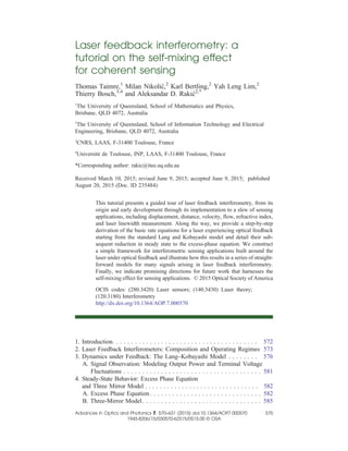
23. in profilometry [116–118]; Fig. 8 depicts recovered amplitude measured across a
vibrating surface. As there is negligible change in feedback strength, C remains
constant, and the expression for the phase stimulus is simply
φst ωsτextt
2πc
λ
2nextLextt
c
4πnextLextt
λ
: (39)
By changing Lext by λ∕2next, which is to say by half a wavelength (taking into
account the refractive index of the external cavity), we change φs by 2π. This
gives rise to a periodicity in the observed signal corresponding to half-
wavelength displacements [119]—“fringes.” Note that the effect of longitudinal
speckle on the interferometric waveform over large distance displacements is
manifested in an additional amplitude modulation envelope; see [94,120,121]
Figure 8
Measured vibration amplitude of a titanium tweeter membrane at 300, 500, 580,
700, 800, 900, 3200, 3500, 3600, 6600, and 6800 Hz, showing different nodal
structures. Reproduced with permission from [118]. Copyright 2014 SPIE.
Advances in Optics and Photonics 7, 570–631 (2015) doi:10.1364/AOP
.7.000570 592
24. for details, and [122–124] for the simultaneous recovery of varying C and for
increased accuracy in the recovered displacement stimulus.
Figure 9 shows typical LFI signals resulting from linear and sinusoidal displace-
ment. The LFI signals show periodicity corresponding to half-wavelength dis-
placements. In the weak feedback regime (that is, C ≤ 1), Eq. (27) has a unique
solution and does not exhibit path dependence—and, in particular, there is no
loss of fringes [see Figs. 9(c) and 9(d)]. Therefore, by recording the interfero-
metric signal [Eq. (30)], we may easily determine the change in external cavity
length relative to λ∕2next by counting the number of whole and fractional
fringes observed [125] or via Fourier transform techniques [126]. If λ is known,
we will have reconstructed the displacement, whose accuracy is fundamentally
Figure 9
Displacement measurement behavior, adapted from [87]. (a), (b) Periodic target
displacement (stimulus) of peak-to-peak amplitude 2λ with λ 850 nm, and
Lext 0.5 m. Linear displacement (blue); sinusoidal displacement (red).
(c)–(j) LFI signals for C 0.5, 5, 8, 25, with α 4.6. Higher feedback levels
exhibit loss of fringes, ultimately resulting in the replication of the stimulus.
Advances in Optics and Photonics 7, 570–631 (2015) doi:10.1364/AOP
.7.000570 593
25. dependent on the wavelength [127]. Resolution can be improved using multiple
reflections on the external target, using, for example, a birefringent crystal
or wave plate inserted in the optical path [128–130]. Using two lasers and
comparing the LFI signals received from them can also be used to improve
resolution [131].
In the moderate and strong feedback regimes (C 1), Eq. (27) has multiple
solutions and exhibits path dependence (see Fig. 4)—and, in particular, may
lead to loss of fringes as feedback increases [see Figs. 9(e)–9(h)]. At very high
levels of feedback, all fringes are lost, and the stimulus is replicated in the
response [see Figs. 9(i) and 9(j)].
As such, the recovery of a stimulus with amplitude ΔLext ≫ λ∕2next from the
measured response (LFI signal) is straightforward only at very high levels of
feedback. As discussed in Section 6.B, it is also straightforward to recover a
stimulus when ΔLext ≪ λ∕2next, regardless of the level of feedback. In all
other cases, recovery of the stimulus can be undertaken, but requires more care;
see [132,133] for details.
Tracking the displacement of the target can be applied to many different appli-
cations, such as sensing the arterial pulse wave in vivo [56] and two-dimensional
tracking of motor shaft displacement [134].
B. Small Displacement Measurement (ΔLext ≪ λ∕2next)
When the target displacement is smaller than λ∕2next, as is the case with small
vibrations, the displacement can still be measured [135–139], but the signal
morphology tends to be different from that in Section 6.A. Suppose that the
length of the external cavity is once again changing as in Eq. (39). For simplic-
ity, consider harmonic variation in external cavity length, Lextt Lext0
jΔLextj sin2πf extt, say, where the maximum displacement satisfies jΔLextj ≪
λ∕2next, varying at frequency f ext. Provided this frequency of vibration f ext is
sufficiently small, we have phase stimulus
φst ωsτext
2πc
λ
2nextLextt
c
4πnextLext0
λ
4πnextjΔLextj sin2πf extt
λ
:
(40)
To obtain good linearity of the stimulus–response transfer function, it is desir-
able to ensure that the small displacements occur within one λ∕2next fringe—
and, in particular, at a quadrature point of the transfer function (see Fig. 10). This
can be achieved by tuning either the lasing frequency ω (through the laser bias
current, I) or the external cavity length Lext0.
In this case, the vibration can be measured in an analog fashion directly from the
interferometric signal, with scale calibrated to within one λ∕2next fringe.
Figure 10 (Visualization 4) explores the dependence of the LFI signal on C.
With increase in C, the slope of the transfer function decreases, bringing about
a corresponding decrease in sensitivity to the stimulus. However, with the in-
creased tilt of the transfer function, its quasi-linear part extends to a larger range
of input phase stimuli, effectively increasing the dynamic range of the sensing
scheme.
This approach also works well with nonharmonic stimulus—see Fig. 11 for an
example of a surface electrocardiographic signal [140].
Advances in Optics and Photonics 7, 570–631 (2015) doi:10.1364/AOP
.7.000570 594
26. C. Measuring Absolute Distance by Linear Frequency
Sweeping
A small variation in laser driving current, ΔI, will produce an approximately
linear variation in the laser operating frequency, Δν. The empirical frequency
modulation coefficient, Ω, relates the two quantities as [141]
Δω 2πΔν 2πΩΔI: (41)
A typical value for Ω for a semiconductor laser diode is −3 GHz∕mA; however,
the exact value for any particular laser must be determined experimentally. With
a fixed external target and a small fractional frequency sweep [Δω∕ωs0 ≪ 1,
so that target reflectivities do not change appreciably over the frequency range
due to material dispersion] we have phase stimulus of
Figure 10
Sinusoidal phase-stimulus–power-response transfer function, with C 2.5 and
α 4.6. Visualization 4 shows the dependence of the LFI signal on C.
Figure 11
Electrocardiographic phase-stimulus–power-response transfer function, with
C 2.5 and α 4.6.
Advances in Optics and Photonics 7, 570–631 (2015) doi:10.1364/AOP
.7.000570 595
27. φst τextωst τextωs0 2πΩΔIt: (42)
The current is typically modulated using a sawtooth or triangle function to
exploit the (approximately) linear relationship between current and frequency.
Note that to achieve a linear frequency shift in practice, some distortion (pre-
emphasis) of the form of the modulating current is usually required [142–144].
Assuming a sawtooth modulation, let us take one period of the sawtooth to be of
the form
ΔIt At; (43)
where A is the slope of the sawtooth function. This corresponds to a phase
stimulus of
φst τextωs0 2πΩAt: (44)
Note that the form of this phase stimulus is functionally identical to that present
in the displacement application discussed earlier. Being a phase stimulus, it will
produce periodic modulation at integer multiples of 2π. By defining the period of
this induced modulation as T, we may write
2π τext2πΩAT; (45)
which gives the optical length of the external cavity as
nextLext
c
2ΩAT
: (46)
Hence, by inducing frequency change at a known rate, one can infer the distance
to the target Lext by fringe counting [125]: Lext cNf 1∕2nextΔω, where
Nf is the number of fringes in the observed interferometric signal. Figure 12
shows a three-dimensional profile reconstructed based on the average frequency
variation between the fringes (see also [145]).
A refinement can be achieved by simultaneously modulating the phase by using
an electro-optic crystal in the external cavity [146]. These coherent schemes
provide high accuracy over a wide range of distances [147]. However, the effect
of longitudinal speckle on the interferometric waveform over large distance dis-
placements is manifested in an additional amplitude modulation envelope; see
[94,120,121] for details.
While fringe-counting is a straightforward method, Fourier transform methods
[in particular, the fast Fourier transform (FFT)] have been shown to provide
superior performance in the presence of noise [148–150]. Moreover, a variant
of tonal analysis, multiple signal classification, has been shown to provide better
performance in the presence of noise than even the FFT [151]. Linear frequency
sweeping has also been used in conjunction with synthetic aperture techniques
and a THz QCL, allowing contrast to be maintained beyond the diffraction
limit [152].
An alternate method for determining absolute distance is to place a chromatic
dispersive element in the external cavity, between the laser and the target. In this
case, the optical feedback from the focal spot on the target is most strongly
coupled back into the laser cavity, providing an LFI signal that corresponds
to the distance between the chromatic dispersive element and the target [153].
Advances in Optics and Photonics 7, 570–631 (2015) doi:10.1364/AOP
.7.000570 596
28. D. Simultaneous Measurement of Distance and Velocity
by Triangular Frequency Sweeping
If the laser current is modulated to produce a periodic triangular frequency sweep
[125], then an estimate of the velocity of the external target is possible at the
same time as an absolute distance measurement [125]. This is made possible
as the increasing linear sweep of frequencies is seen interferometrically as a
linear extension of the external cavity, while the decreasing linear frequency
sweep is seen as a linear contraction of the external cavity. As such, the number
of interferometric fringes on the increasing and decreasing sweeps gives informa-
tion about the location and change in location of the external target itself.
Figure 13 depicts the two physical stimuli (linear displacement and triangular
frequency sweep), which combine into a single phase stimulus. The typical LFI
signal (response) in this case is shown in Fig. 13(c), from which fringes on the
increasing and decreasing portions of the frequency sweep may be extracted—
for example, by numerical differentiation [see Fig. 13(d)]. These fringe counts
contain information about the location and change in location of the external
target.
E. Measuring Change of Refractive Index in External
Cavity
A change in the (real-valued) refractive index of the external cavity is effectively
a change in the optical length of the external cavity, and is thus equivalent to
Figure 12
Three-dimensional range image of a bottle of corrector fluid against a flat back-
ground acquired at a distance of 0.7 m. The bottle height is 71 mm, and its
diameter is 27 mm. (c) IEEE. Reproduced, with permission, from Gagnon
and Rivest, IEEE Trans. Instrum. Meas. 48, 693–699 (1999) [141].
Advances in Optics and Photonics 7, 570–631 (2015) doi:10.1364/AOP
.7.000570 597
29. changing the geometrical length of the cavity, as in Sections 6.A and 6.B. An
interesting example is the imaging of acoustic fields (see Fig. 14). We may write
the phase stimulus as
φst ωsτextt
2πc
λ
2nexttLext
c
4πnexttLext
λ
: (47)
For large phase changes, in a similar way to displacement measurement, changes
in external cavity refractive index can be detected simply by fringe counting,
Figure 13
LFI response to simultaneous linear displacement and frequency changes.
(a) Linear displacement (constant velocity of 10 mm/s). (b) Triangular frequency
sweep (2 GHz peak-to-peak on λ0 850 nm). (c) Typical LFI signal (C 0.9
and α 4.6)—note the presence of large power modulation as a consequence of
laser current (and hence output power) modulation. (d) Numerically differenti-
ated LFI signal, showing differing number of fringes over the increasing portion
of the frequency sweep and the decreasing portion of the frequency sweep.
Adapted from [87].
Advances in Optics and Photonics 7, 570–631 (2015) doi:10.1364/AOP
.7.000570 598
30. with improved resolution possible by arrangement of a series of external mirrors
guiding the laser beam multiple times through a sample placed in the external
cavity [35]. Small phase changes can be detected by automatic calibration at a
series of three, four, or five settings of an electro-optic modulator inserted into
the external cavity [155,156].
Alternately, when the emitted beam is coupled into an external fiber, strain
applied to the fiber results in changes in both external cavity length and its re-
fractive index, permitting the integral strain along the fiber to be measured
[157,158]. Another interesting recent application is the sensing of trace gas
in the external cavity [159,160].
Figure 14
Propagation of the acoustic field with the ultrasonic transmitter propagating the
field into free space. Left, measured; right, simulation. (a) Image at t 0 s.
(b) Amplitude of acoustic field. (c) Phase of acoustic field. Reproduced with
permission from [154]. Copyright 2014 Optical Society of America.
Advances in Optics and Photonics 7, 570–631 (2015) doi:10.1364/AOP
.7.000570 599
31. 7. Target-Related Measurement
A. Measuring Material Complex Refractive Index of the
Target by Slow Linear Frequency Sweeping: Material
Characterization
As in Section 7.D, the optical length of the external cavity nextLext is held con-
stant, and the temporal variation in complex refractive index of the target is
under investigation. To measure the complex refractive index of the target
(rather than its temporal change) one can slowly sweep the laser frequency, en-
abling the extraction of the complex refractive index of the target material. The
amplitude and phase of the reflection coefficient of the target are as in Eqs. (53)
and (54), but the linear frequency sweep (similar to Section 6.C) modifies the
inputs to the excess phase equation as
φst ωstτext − θR
2nextLextωs0
c
2nextLextjΔωjt
c
− θR: (48)
In Eq. (48), an emitted wave takes time τext∕2 to traverse the external cavity,
accumulating transmission phase; is reflected from the (stationary) external tar-
get, which imparts phase shift on reflection θR; and returns to the laser, once
again taking time τext∕2 to traverse the external cavity, accumulating transmis-
sion phase. The offset of the interferometric waveform due to the linear fre-
quency sweep shifts depending on the phase shift on reflection from the
target, while the amplitude of the waveform depends on the reflectivity of
the target. This pair of target characteristics is related to its refractive index
(n) and extinction coefficient (k), which can therefore be recovered by calibrat-
ing the system with respect to known reference materials [54,161]. Even without
calibration, this enables the concurrent mapping of amplitude and phase infor-
mation of the external target, providing two registered images of the target,
which could then be used to build up its three-dimensional profile. For example,
Fig. 15 shows the imaging of porcine tissue obtained using LFI. However, this
type of sensing scheme has to date been demonstrated only with THz QCLs at
cryogenic temperatures [54,162,163], and it remains to be seen whether other
types of lasers (that may be less stable due, for example, to thermal effects or
laser phase noise [164]) are appropriate for this sensing scheme.
B. Imaging by Frequency Shifting Using Acousto-Optic
Modulators
An acousto-optic modulator may be used to frequency shift laser emission for
imaging and sensing purposes [165]. This has the advantage of not altering the
laser operating state, as is the case when employing a current sweep. This tech-
nique is often used for imaging as in, for example, biomedical imaging using
confocal microscopy [166] or confocal fiber laser imaging of waveguide modes
[22], but it can be applied in a wide range of LFI settings. Figure 16 shows some
interesting imaging results from these. Acousto-optic techniques can also be
used to reduce the effect of parasitic reflections, i.e., from microscope slides
[167], and to reach the shot noise limit with mirror scanning [168].
Advances in Optics and Photonics 7, 570–631 (2015) doi:10.1364/AOP
.7.000570 600
32. C. Measuring Thickness and Refractive Index of a
Transparent Material
An interesting application of LFI is the simultaneous measurement of thickness
and refractive index of a transparent material [169]; see Fig. 17. A related ap-
proach to measuring the refractive index of a transparent material may be found
Figure 15
Terahertz porcine tissue imaging using LFI. (a) Amplitude-like imaging modal-
ity based on a 101 × 101 array of LFI waveforms (inset: high-resolution image
based on a 51 × 301 array), and (b) the phase-like imaging modality. (c)–(h)
Heat maps of LFI waveforms for different tissue types associated with the color
markers overlayed in (a). The tissue types are: (c) aluminum separator, (d) epi-
dermis, (e) upper dermis, (f) lower dermis, (g) sub-dermal fat, and (h) muscle
tissue. (i) Corresponding amplitude-like/phase-like plots of waveforms (c)–(h).
The mark of each tissue type appears to form natural clusters. Reproduced with
permission from [162]. Copyright 2014 Optical Society of America.
Advances in Optics and Photonics 7, 570–631 (2015) doi:10.1364/AOP
.7.000570 601
33. in [170]. This technique uses two concurrently monitored interferometric signals
in the weak feedback regime: (1) the interferometric signal at PD2 (resulting
from interference of the transmitted and double-reflected beam), and (2) the
interferometric signal at PD1. The phase difference between the transmitted
and the double-reflected beam is
ΔφPD2 2knd cos θ; (49)
where n is the refractive index of the transparent sample, d is sample thickness,
θ is the angle of refraction at the first sample interface, and k 2π∕λ is the
(free-space) wave number. In addition to depending on θ, the change in phase
stimulus at PD2 also depends on the angle α at which the sample is offset from
the beam-axis normal, as
ΔφPD1 2kdn cos θ − cos α: (50)
Figure 16
(a) (b)
(c) (d)
(a) Photograph of Egyptian doll head, reproduced with permission from [165].
Copyright 2001 Optical Society of America. (b) 3D image of the doll head from
(a), obtained by imaging using an acousto-optic modulator, reproduced with per-
mission from [165]. Copyright 2001 Optical Society of America. (c) Phase image
of an isolated red blood cell on a glass slide, obtained by acousto-optic imaging,
reprinted from Ultramicroscopy 111, Hugon et al., “Coherent microscopy by laser
optical feedback imaging (LOFI) technique,” 1557–1563 (2011), with permission
from Elsevier [166]. (d) Phase map of light propagating along the waveguide,
reprinted with permission from [22]. Copyright 2008 Optical Society of America.
Advances in Optics and Photonics 7, 570–631 (2015) doi:10.1364/AOP
.7.000570 602
34. The difference between these two,
ΔφPD2 − ΔφPD1 2kd cos α; (51)
is independent of refractive index n of the material. Hence, measurement of
phase difference dependence in Eq. (51) with α will yield thickness d. Once
d is known, the dependence of ΔφPD2 in Eq. (49) on refraction angle θ permits
a crude estimate for n.
D. Measuring Change in Target Refractive Index
For this application, the external cavity length and its refractive index are con-
stant. An example is the measurement of a fiber Bragg grating under strain [171].
Now consider the target to have a (complex) refractive index ñ n − jk, where
the negative sign is once again a consequence of the convention to use e jωt
in
describing the temporal dependence of the wave. Assuming normal incidence
from a lossless medium onto an optically thick target (half-space), the target
amplitude reflection coefficient is [172]
r
next − ñ
next ñ
next − n jk
next n − jk
: (52)
Taking the convention r jrje jθR , the amplitude, jrj, and phase, θR of the
reflection coefficient are
jrj
ffiffiffiffiffiffiffiffiffiffiffiffiffiffiffiffiffiffiffiffiffiffiffiffiffiffiffiffiffiffiffiffi
next − n2
k2
next n2
k2
s
(53)
θR Arctan2nextk; n2
ext − n2 − k2; (54)
where Arctany; x denotes the four-quadrant arctangent function of a vector with
Cartesian coordinates x; y.
Figure 17
Apparatus for the simultaneous measurement of thickness and refractive index
of a transparent material (adapted from [169]). The emitted beam is incident to
the transparent sample at angle α and is refracted at angle θ to the partial reflector
and second photodetector (PD2). A portion of the beam is reflected and sub-
sequently returns to the laser diode, whose optical power is monitored by
the first photodetector (PD1). A part of this returning beam undergoes reflection
from the internal surface of the sample, resulting in double reflection. This dou-
ble-reflected beam is observed only at PD2 and has negligible impact at PD1.
Advances in Optics and Photonics 7, 570–631 (2015) doi:10.1364/AOP
.7.000570 603
35. When n next—for example, when the beam is incident from air and probing a
higher index material—we have k ≥ 0 and n next, and Eq. (54) will give a θR
in the second quadrant of the complex plane. Using the standard definition of
the arctan function, which has range −π∕2; π∕2—that is the first and fourth
quadrants—we may write
θR arctan
2nextk
n2
ext − n2
− k2
π: (55)
If the material extinction coefficient k is zero, then the phase change is simply π
as expected. Note that we may have n next—for example, when the beam is
incident from a fiber probing a lower index lossy material.
Therefore, changes in complex target refractive index will induce changes in
both the amplitude and phase of the reflected optical wave. As C is directly
proportional to jrj [via Eqs. (1) and (2)], changes in jrj will change C by a pro-
portional amount. Changes in θR will change φs by an equivalent amount.
Explicitly, this results in phase stimulus of
φst ωsτext − θRt
4πnextLext
λ
− θRt; (56)
and amplitude stimulus of
Ct C0
jrtj
jr0j
: (57)
A scheme of this nature was used recently to image free carriers in semiconduc-
tors using a THz QCL [173] (see Fig. 18). Another interesting recent application
is to measuring thin layers of residues on surfaces [174].
E. Alignment and Angle Measurement of Remote Target
When the external target is at a fixed distance from the laser, but possibly mis-
aligned (in the angular sense) [175,176], its effective (complex) amplitude
reflection coefficient can be viewed as a function of its two angular deflections
(θ and ϑ, say) from the plane transverse to the laser beam, as
rθ; ϑ jrθ; ϑje jθR ; (58)
resulting in phase stimulus (explicitly highlighting phase-shift on reflection) of
φst ωsτext − θR
4πnextLext
λ
− θR; (59)
and angle-dependent characteristic feedback parameter C, as
Cθ; ϑ C0; 0
jrθ; ϑj
jr0; 0j
: (60)
When the effective target reflectivity in the direction of the beam axis decreases
with departure from perfect alignment, as is the case for many external targets,
including for minor mirror misalignment, this angular dependence provides
means for target alignment and therefore angle measurement. By creating an
Advances in Optics and Photonics 7, 570–631 (2015) doi:10.1364/AOP
.7.000570 604
36. interferometric signal (for example, by simply chopping the laser beam), adjust-
ing the two angles until maximum peak-to-peak signal is achieved will corre-
spond to a well-aligned target. Indeed, this idea has been used to investigate
the effect of optical feedback due to Fresnel reflections from a fiber front end in
characterizing laser-to-fiber coupling techniques [177]. When the target can be
displaced, an alternative approach that exploits the stimulus replication phenome-
non of the phase-insensitive coherence collapse regime can be found in [175].
One can also employ three laser sensors operating with sawtooth frequency
stimulus to measure displacement at three points on the target, thereby recov-
ering angular rotation [176].
F. Intensity-Based Measurement
While the many applications of LFI discussed previously rely on the coherent
(phase-based) information contained in the LFI signals, for some applications it
is desirable or unavoidable to forgo this coherent information and instead rely on
the intensity-based information contained in the optical feedback. Laser Doppler
velocimetry for rough surfaces and fluid flow is one application discussed in
Figure 18
(a)
(b)
(a) Representative intensity distributions of the infrared pump laser by placing a
charge-coupled device (CCD) camera at the sample position. The pattern was
computer controlled by a spatial light modulator (SLM) and projected onto the
silicon surface. Dark pixels of SLM liquid crystal maintain the polarization of
the incident light and define the exposed area. (b) Terahertz imaging in reflection
mode of photoexcited electron plasma on semiconductors. The spatial distribu-
tion of free carrier charges corresponds to the structured beam profile. Reprinted
with permission from Mezzapesa et al., Appl. Phys. Lett. 104, 041112 (2014)
[173]. Copyright 2014 American Institute of Physics.
Advances in Optics and Photonics 7, 570–631 (2015) doi:10.1364/AOP
.7.000570 605
37. more detail in Section 7.G. Another interesting application is the profiling and
imaging of surfaces using LFI in a confocal microscope configuration
[78,91,178,179] (see Figs. 19, 20, and 21).
In these instances, the laser is operated at a constant bias current, and simply the
change in bias current due to optical feedback is recorded. This change can be
directly related to the change in surface profile [91].
A further application is as follows. If the phase information is randomized by
reflection from a rough surface, or is otherwise discarded, relative measurement
of the target’s reflectivity is possible simply though monitoring the peak-to-peak
Figure 19
(a), (b) Two specimen through-focus images of a semiconductor chip taken at
3 μm axial separation with a semiconductor laser confocal microscope. Field of
view is 80 μm × 80 μm. Reprinted with permission from [78]. Copyright 1994
Optical Society of America.
Figure 20
Locating defective transistors using an optical-feedback thermographic micro-
scope. (a) Thermal map of photodetector array sample superimposed on refer-
ence confocal image showing anomalous “hotspots” (yellow regions), which are
possible defect sites. (b) Regions of increasing thermal activity reveal the integ-
rity of the semiconductor architecture where thermal blooming on two regions is
apparent. Image area is 180 μm × 180 μm. (c) Homogeneity of the localized
quantum efficiency of regions across a silicon photodiode is evaluated at optical
spatial resolution. Region 1 represents a substrate; 2, n-type semiconductor; 3,
p–n overlay; and 4, bonding pad. (d) Thermal map of the quantum efficiency of
the photodiode revealing the nonuniform response on the boundaries and the n
region. Image area is 270 μm × 270 μm. Reprinted with permission from [179].
Copyright 2006 Optical Society of America.
Advances in Optics and Photonics 7, 570–631 (2015) doi:10.1364/AOP
.7.000570 606
38. LFI signal amplitude. Translating rough surfaces at a known velocity permits their
characterization by monitoring the fluctuations in effective reflectivity [182].
G. Doppler Velocimetry and Flow Imaging
This sensing scheme—LFI velocimetry—is based on the well-known Doppler
effect that dictates that a moving object will impart a frequency shift to light
incident upon it. In this sensing scheme, the Doppler beat frequency of the in-
terferometric signal is observed, just as in a standard laser Doppler velocimeter
(LDV) [183]. The scheme differs from LDV in that the self-mixing effect will
introduce nonlinearity into the signal and the scheme requires no reference arm.
At first glance, it may seem that LFI velocimetry is a simple matter—one simply
observes the beat frequency induced by the Doppler effect and thereby deduces
the velocity of the target. However, a more careful consideration of this sensing
Figure 21
Intensity-based (chopped beam) LFI imaging of coins. (a) A British two-pence
coin. (b) A high-resolution image of (a) using a THz QCL operating at 2.60 THz.
(c) An Australian five-cent coin. (d) An image of (c) using a 3.57 μm mid-
infrared DFB interband cascade laser. (e) An image of (c) using an 851 nm
near-infrared VCSEL. Adapted from [21,180,181].
Advances in Optics and Photonics 7, 570–631 (2015) doi:10.1364/AOP
.7.000570 607
39. scheme reveals many subtleties and gives a deeper understanding of LFI in
general.
1. Principle of Operation
The Doppler shift, Δf , incurred by light upon scattering by an object with the
velocity vector v is [183]
Δf
1
2π
ks − ki · v; (61)
where ks and ki are the scattered and incident wavevectors. Assuming direct
backscattering reduces Eq. (61) to
jΔf j
1
π
ki · v
2nv cosθ
λ
; (62)
where v ‖v‖, θ is the angle between the laser beam axis and the target velocity
vector, n is the refractive index of the medium surrounding the target, and λ is the
laser emission wavelength in vacuum. This simplified equation works well in
practice, as the scattered light must return to the laser in order to contribute to the
LFI signal (monostatic geometry) [53,103].
It is instructive to consider Eq. (61) in more detail. Figure 22 depicts a ray of
light with incident wavevector ki impinging on an optically flat surface. We see
clearly that the vector quantity ks − ki is normal to the surface tangent plane. In
order to have a non-zero Doppler shift, Eq. (61) demands that the vector dot
product ks − ki · v be non-zero. This means that the velocity vector must
be outside the surface tangent plane for a Doppler shift to occur. That is, the
surface must be translating in such a way as to change the external cavity length.
If the cavity length is not changing (i.e., the velocity vector is in the plane tan-
gent to the surface), no Doppler shift occurs.
Figure 22
Visualization of Eq. (61). The vector ks − ki is normal to the reflection surface.
If the velocity vector v is in the plane tangent to the reflection surface, as pic-
tured, there will be zero Doppler shift. A velocity vector outside this plane will
give a non-zero Doppler shift, which means the surface is translating in such a
way that it is changing the external cavity length. Therefore, the external cavity
length must change for a Doppler shift to occur.
Advances in Optics and Photonics 7, 570–631 (2015) doi:10.1364/AOP
.7.000570 608
40. To illustrate this, consider the case of a rotating (but otherwise stationary) disk. If
the surface of the disk has flatness sufficiently smaller than the laser emission
wavelength such that specular reflection is dominant (i.e., it is optically flat),
Eq. (61) gives zero Doppler shift regardless of the incident wavevector’s direc-
tion, as ks − ki will always be normal to the velocity vector. The mathematics
here is clear, but the authors also confirmed this experimentally by coupling the
reflected light from a disk of this nature back into the laser; no Doppler shift was
observed.
Now let us consider the same disk, but with surface roughness significant com-
pared to the laser wavelength. As the disk spins, its roughness modulates the
external cavity length. Analyzing the statistics of the reflection process is beyond
the scope of this article, but one may intuitively reason that the mean Doppler
shift is given simply by the component of the target velocity vector along the
laser beam axis, and this is indeed observed in experiment [103]. That is to say,
the mean Doppler shift is given by Eq. (62). These two cases (an optically
smooth and a rough disk) illustrate the principle derived through solely math-
ematical considerations above—cavity length must change for a Doppler shift to
occur. In fact, LFI Doppler velocimetry is equivalent to displacement measure-
ment (covered in Section 6.A). This equivalence has been noted even for the
more general case of laser Doppler and laser speckle velocimetry [184]. LFI
displacement counts fringes corresponding to λ∕2 displacement, whereas LFI
velocimetry considers the frequency of those same fringes (i.e., the Doppler
frequency) and thereby infers the target velocity.
Surface roughness will inevitably lead to speckle effects [185]. Just as for dis-
placement measurement, speckle can have a detrimental effect on systems
tracking the motion of rough targets, as the “dark speckles” caused by destruc-
tive wave interference will attenuate the LFI signal. This negative effect can be
ameliorated by implementing a real-time signal tracking algorithm [94,186], or
by physically moving a lens with piezo-actuators [187].
Fully developed speckle will destroy phase coherence—the beam reflected from
a rough surface will have uniformly random phase on 2π [185]. This does not,
however, stop the beam from accruing a Doppler shift. When approaching LFI
velocimetry from the speckle perspective, the autocorrelation function is typi-
cally used to analyze the LFI signal [188]. When approaching the problem from
the Doppler perspective, the power spectrum is typically used to analyze the
signal, which is simply the Fourier transform of the autocorrelation function
by the Wiener–Khintchine theorem [185]. Therefore, both approaches are valid
and fundamentally linked. We choose to proceed using the Doppler approach,
and analyze the signal by considering its power spectrum.
Finally, one may wonder how it is possible to detect a Doppler shift, frequently
in the kilohertz range, far below the typical laser diode linewidth (some tens of
megahertz). This dilemma was solved in the field of radar Doppler [189,190]—
the emitter (the laser in our case) is considered as a fixed-frequency source with a
LFI Doppler velocimetry, speckle velocimetry, and displacement
measurement are all fundamentally the same. External cavity length
must change in order for a Doppler shift to occur.
Advances in Optics and Photonics 7, 570–631 (2015) doi:10.1364/AOP
.7.000570 609
41. certain phase noise (corresponding to the laser linewidth). As the phase of the
reinjected electromagnetic field is statistically correlated to some degree with the
phase of the laser emission, the frequency noise in the “baseband” is severely
attenuated, an effect termed range correlation. This allows the observation of
Doppler shifts far below frequencies corresponding to the laser linewidth.
2. Modeling
Modeling the LFI velocimetry signal is done in two parts—the light–target in-
teraction and the laser dynamics. The nature of the target and the optical system
will dictate the light–target interaction and the ensuing Doppler-shift distribution
that will re-enter the laser cavity and be subject to the laser dynamics.
A body in motion, such as a rough, rotating disk, exhibit a Gaussian peak in the
spectrum centered about the Doppler frequency expected from the velocity at the
center of the laser spot [103]. Increasing the numerical aperture of the beam
incident on the target will broaden the spectrum and vice versa [191].
The Doppler-shift spectrum for fluids is complicated by scattering effects. If the
fluid is weakly scattering—i.e., each photon is most likely to be scattered once or
not at all—then the spectrum tends to resemble that of a rough body in motion
[53]. Figure 23(a) shows representative spectra for a range of flow rates at the
same (weak) scattering level using external optics to focus the beam at the center
of the flow channel.
If the fluid is strongly scattering, as is often the case for blood flow measurement
[192], then the spectrum does not exhibit a clear Doppler peak, but rather a dis-
tribution governed by the statistics of the scattering process [52,193]. Models for
the Doppler-shift spectrum have been reported, taking into account scattering
effects [52,194–196].
To model laser dynamics, an inverse FFT method may be used to transform the
Doppler-shift spectrum into a complex time series ψt (taking care to assign
each frequency component uniformly random phase for the case of fully devel-
oped speckle). Then we may write the phase and amplitude stimuli as [87]
φst ωsτext argψt (63)
Figure 23
Morphology of Doppler flow spectra, adapted from [53,55]. (a) Doppler flow
spectra for six flow rates ranging from 0 to 50 μL/min for the same scattering
level of 2% wt. % milk diluted in water. (b) Doppler flow spectra for four scat-
tering levels, ranging from 0.2% to 100% wt. % milk diluted in water, for the
same maximum fluid velocity of 1.6 mm/s.
Advances in Optics and Photonics 7, 570–631 (2015) doi:10.1364/AOP
.7.000570 610
42. C C0jψtj; (64)
where C0 is the constant, nominal value of C. As the fractional change in the
laser operating frequency due to the Doppler effect is very small, ωs may be
considered to remain constant. It should also be noted that here τext is a constant,
nominal value for the external cavity round-trip time.
The nonlinear process of LFI produces harmonics, and, as such, measurement is
ideally performed under weak feedback, though monitoring the ratio of power of
the peak Doppler frequency to its second harmonic gives a measure of feedback
level [197].
3. Spectral Analysis and Velocity Extraction
The spectral analysis of the LFI signal is commonly carried out by application
of the FFT; however, it has been shown that multiple signal classification, a
frequency estimator using a single a priori parameter, provides improved
performance in the presence of noise and obviates the need for fitting for
Gaussian spectral distributions [151,198].
In this case, the average flow can be extracted by finding the frequency at which
the signal spectrum intersects the noise floor [199], by considering the first mo-
ment of the spectrum [200], or by tracking the frequency at which the spectral
power is reduced from its maximum by a fixed amount [55]. The optical system
configuration will also necessarily affect the spectrum [191], and may cause the
signal spectrum to be non-Gaussian even for weakly scattering fluids [55].
Figure 23(b) shows representative spectra for a range of scattering levels at
the same flow rate.
4. Flow Imaging and Other Applications
The above technique can be applied in many interesting situations. In 1984, de
Mul et al. [200] measured the velocity of blood flow in a tube and in vivo on
human skin using an external laser. Koelink et al. [199] inserted an optical fiber
into a glass tube to measure the velocity of polystyrene spheres in water as well
as human blood. Özdemir et al. [201] measured velocity of blood flow in vitro in
a 5 mm channel and in vivo in human fingertips and wrists using a laser and a
lens at a distance from the target. Lim et al. [104] demonstrated an LFI flow
sensor using a VCSEL array, imaging fluid velocity in a planar flow channel
of 3 mm thickness. Figure 24 shows the experimental and theoretical flow im-
ages of the channel. Norgia et al. [52] performed experimental and theoretical
studies of sensing the velocity of extracorporeal blood flow in a 9 mm diameter
channel. Campagnolo et al. [53] measured the spatial flow profile of Newtonian
and non-Newtonian fluids within a 320 μm channel using external optics.
Nikolić et al. [55] demonstrated an LFI flowmeter using an optical fiber em-
bedded within a microfluidic structure.
The shape of the Doppler spectrum induced by Brownian motion of a fluid at rest
can be used to measure particle size within the fluid, as scatterers of different
sizes will have a different spatial scattering profile [202–204].
The measurement of wind speed by LFI is a related application in which light is
scattered from particulates in the air, much as light is scattered by particles in
fluid as above [205].
Advances in Optics and Photonics 7, 570–631 (2015) doi:10.1364/AOP
.7.000570 611
43. 8. Laser-Cavity-Related Measurement
A. Laser Linewidth and Linewidth Enhancement Factor
(α) Measurement
The susceptibility of laser linewidth to optical feedback has long been studied
[67,206]. Indeed, the measurement of laser linewidth and linewidth enhance-
ment under feedback is a mainstay of LFI [19,20,207–213]. It is important
to keep in mind that the linewidth and Henry’s linewidth enhancement factor
α under feedback often depend on the laser biasing condition, as well as the
level of optical feedback [213]. The values reported for α vary a great deal be-
tween different device structure and measurement technique—investigation into
which factors influence α is a topic of ongoing investigation [213].
Experimentally determining α by LFI may be achieved in a number of ways. The
phase-stimulus–power-response transfer function (i.e., see Fig. 10) strongly
depends on C and α. In the moderate feedback regime, where multiple solutions
exist and the interferogram (the LFI signal) exhibits hysteresis, the hysteresis
observed in the LFI signal can be linked to the transfer function, and hence
to C and α [214]. The advantage of this method is that no high-frequency or
optical spectrum measurements are required, and the reported accuracy of
determining α is 6.5%. Alternatively, direct fitting of the experimental LFI
signal to theory can be employed [207], or a multiple-parameter optimization
Figure 24
V−Position
(mm)
Simulated
0 5 10 15 20 25 30
−8
−4
0
4
8
H−position (mm)
V−Position
(mm)
Measured
Flow speed (mm/s)
0 5 10 15 20 25 30
−8
−4
0
4
8
0 1 2 3 4
Simulated and measured distribution of velocity components along the lasing
axes for a flow channel with inlet (at left) flow rate of 15 ml/min. Reprinted
with permission from [104]. Copyright 2010 Optical Society of America.
Advances in Optics and Photonics 7, 570–631 (2015) doi:10.1364/AOP
.7.000570 612