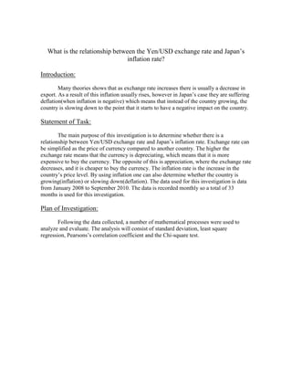
1. What is the relationship between the Yen/USD exchange rate and Japan’s inflation rate?<br />Introduction: <br />Many theories shows that as exchange rate increases there is usually a decrease in export. As a result of this inflation usually rises, however in Japan’s case they are suffering deflation(when inflation is negative) which means that instead of the country growing, the country is slowing down to the point that it starts to have a negative impact on the country.<br />Statement of Task:<br />The main purpose of this investigation is to determine whether there is a relationship between Yen/USD exchange rate and Japan’s inflation rate. Exchange rate can be simplified as the price of currency compared to another country. The higher the exchange rate means that the currency is depreciating, which means that it is more expensive to buy the currency. The opposite of this is appreciation, where the exchange rate decreases, and it is cheaper to buy the currency. The inflation rate is the increase in the country’s price level. By using inflation one can also determine whether the country is growing(inflation) or slowing down(deflation). The data used for this investigation is data from January 2008 to September 2010. The data is recorded monthly so a total of 33 months is used for this investigation.<br />Plan of Investigation:<br />Following the data collected, a number of mathematical processes were used to analyze and evaluate. The analysis will consist of standard deviation, least square regression, Pearsons’s correlation coefficient and the Chi-square test.<br />Table 1: Yen/USD Exchange rate and Japan’s Inflation rate over 33 months<br />Time when data is collectedYen/USD Exchange Rate(¥/$)Japan's Inflation Rate(%)Jan-08107.81810.7Feb-08107.03001.0Mar-08100.75621.2Apr-08102.67770.8May-08104.35951.3Jun-08106.91522.0Jul-08106.85182.3Aug-08109.36242.1Sep-08106.57482.1Oct-0899.96591.7Nov-0896.96561.0Dec-0891.27500.4Jan-0990.12050.0Feb-0992.9158-0.1Mar-0997.8550-0.3Apr-0998.9200-0.1May-0996.6445-1.1Jun-0996.6145-1.8Jul-0994.3670-2.3Aug-0994.8971-2.2Sep-0991.2748-2.2Oct-0990.3671-2.5Nov-0989.2674-1.9Dec-0989.9509-1.7Jan-1091.1011-1.3Feb-1090.1395-1.1Mar-1090.7161-1.1Apr-1093.4527-1.2May-1091.9730-0.9Jun-1090.8059-0.7Jul-1087.5005-0.9Aug-1085.3727-0.9Sep-1084.3571-0.6<br />The data of the exchange rate is left at 4 decimal places for the sake of increased precision and accuracy. Also due to the fact that exchange rate is usually kept at 4 decimal places. Also even though some of the inflation rate data is negative it is still considered as inflation, specific term deflation, however as to simply things, the title is kept as inflation.<br />34290501650Graph 1: This graph shows the raw data plotted onto a scatter plot. There seems to be a slight positive correlation. The degree of strength is not known as of this moment.<br />To find the degree of the correlation other equations will be used to help out. Some equation for the sake of simplicity will show a basic demonstration of how to find the result. This will be mention later as needed.<br />Standard Deviation Calculations<br />Standard deviation measures the variability/dispersion of the particular variables. Shown by the following equation. (note that there is 2 equations, used for the why x and y axis.)<br />Sx=Σx2n-x2Sy=Σy2n-y2Component of standard deviation consist of the sum of all the numbers within a column squared, represented by the sigma sign. Also the number of variables within each column, in this case being represented by n, however the data will not be increasing so for this situation, n=33 for both y and x. The mean value of x and y is found by using the equation<br />Average=sum of all numbersamount of numbers used to find the sum<br />The actual sample calculations will not be done since the number of data would cause it to be longer then necessary. So as a result the numbers have been founded through the use of Microsoft word excel.<br />x= 96.03531515y= -0.251515152<br />x≈96.0353y≈-0.25<br />Exchange rate is once again kept at 4 decimal places for accuracy. However when used in equation the exact number will be used in the equations.<br />Sx=305969.833-96.0352<br />Sx=9271.81323-9222.781756<br />Sx=49.03147<br />Sx=7.002247806<br />Sx≈7.0023<br />Standard deviation of x is 543 which means that the data is extremely disperse, meaning that the data are really far away from the mean.<br />Sy=68.8933-.0632598714<br />Sy=1.422784554<br />Sy≈1.42<br />Standard deviation of y is 1.42 which means that the data is disperse, but still close to the mean to an extent. Which means the data are at the same time somewhat grouped together.<br />Least Square Regression<br />Least Square Regression calculations identify the relationship between the independent variable,x, and the dependant variable,y. The least squares regression is given by the following formulas:<br />y-y=SxySx2x-x Which can be derived into Sxy=Σxyn-xy<br />Sxy=-548.1806433-96.03531515-0.251515152<br />Sxy=(-16.61153455)-(-24.1543)<br />Sxy=7.542802<br />Sxy=7.54<br />Therefore<br />y--0.251515152=7.5428027.002252x-96.03531515<br />y--0.251515152=0.153836x-96.03531515<br />y=0.1538x-14.77367-0.251515152<br />y=0.1538x-15.02519<br />y≈0.154x-15.0<br />y≈0.154x-15.0 is the least square regression formula for this particular set of data. This is shown later on graph 2 which shows the result.<br />Pearson’s Correlation Coefficient<br />Pearson’s correlation coefficient indicates the strength of the relationship between the two variables. It is given by the following equation:<br />r=SxySxSy<br />r=7.542802543.25778067.0022478711.422784554<br />r=.75915<br />r2=.5763<br />r2≈.576<br />Graph 2:<br />This graph is the same as the previous graph except that it has been fitted with a line of best fit using the equation: y≈0.154x-15.0 By looking at the line of best fit, it can be assumed that there is a moderately positive linear correlation between Japan’s inflation rate and Yen/USD Exchange rate. The positive linear relationship can also be figured out from the Pearson’s Correlation Coefficient Value, which is r2=.5763 by comparing this with the table value one can see the moderate correlation.<br /> χ2 Test of Independence<br />χ2 test of independence measures the independence of the two variables and whether the occurrence of one of them affect the occurrence of the other. The formulas used to show χ2 are shown below:<br />Observed Values:<br />B1B2TotalA1aba+bA2cdc+dTotala+cb+dN<br />Calculations of Expected Values:<br />B1B2TotalA1a+ba+cNa+bb+dNa+bA2a+cc+dNb+dc+dNc+dTotala+cb+dN<br />χ2=Σobserved value-expected value2expected value<br />Degrees of freedom measures the number of values in the calculation that can vary:<br />Degrees of Freedom=rows-1(column-1)<br />Null (H0) Hypothesis: Yen/USD Exchange rates and Japan’s Inflation rates are independent.Alternative (H1) Hypothesis: Yen/USD Exchange rates and Japan’s Inflation rate are not independent.<br />Table 2: Observation Value<br />Inflation Rate-2.5<x<0Inflation Rate0.1<x<2.6TotalExchange Rate 84<x≤9719221Exchange Rate97<x≤11021012Total211233<br />This is the data from Table 1 in which it has been categorized into a wide range so that it is simpler and does not interfere with data calculations later on.<br />Table 3: Calculations for Expected Values<br />Inflation Rate-2.5<x<0Inflation Rate0.1<x<2.6TotalExchange Rate 84<x≤9721213321123321Exchange Rate97<x≤11012213312123312Total211233<br />This shows how the data was calculated for Table 4 shown below. <br />Table 4: Expected Value<br />Inflation Rate-2.5<x<0Inflation Rate0.1<x<2.6TotalExchange Rate 84<x≤9713.363647.63636421Exchange Rate97<x≤1107.6363644.36363612Total211233<br />The numbers is kept in more than 3 significant figures for a more accurate and precise data. The numbers has been left according to the figures shown on excel.<br />χ2=19-13.36364213.36364+2-7.63636427.636364+2-7.63636427.636364+10-4.36363624.363636<br />χ2=17.97789<br />χ2≈18.0<br />Degrees of Freedom=2-1(2-1)<br />Degrees of Freedom=1<br />The χ2critical value at 5% significance with 1 degree of freedom is 3.841and with 1% significance is 6.635. The result from the χ2 test shows an 18.0 which means that the result is greater than the critical value, therefore, the null(H0) hypothesis is rejected. Due to the null hypothesis being rejected, the alternative hypothesis would have to be accepted. This would mean that Yen/USD Exchange rates and Japan’s Inflation rate are not independent.<br />Discussion:<br />Data interpretation:<br /> Graph 1 shows the disperse data without a linear fit, but later on in Graph 2 a linear fit line was placed in. This is use to show the data before and after the placement of the linear fit. The linear fit was figured by using the Pearson’s Correlation Coefficient, by using this r2, and the table we can see that there is a moderately positive relationship. As a result, this shows that Japan’s inflation rate may have had an effect on exchange rate. However this is not certain since there may have been other factors involve that may have affected the data.<br /> Also since the χ2 test showed that the Japan’s inflation rates and Yen/USD exchange rates are dependant of each other, this proves that there is indeed a relationship, since if they are dependant, an increase in one of the variable would, ceteris paribus, increase the other variable. This shows that they are related in a positive way, since an increase in one variable, would cause an increase in the other variable. <br />Limitations:<br /> Table 1 shows all of the data from the 33 months. One major limitation that should be noted as part of the discussion is that, the actual date the data was taken in. Since inflation rate data could have been taken at the beginning of the month, and exchange rate could have been taken at the end of the month, this would then cause a lag time to occur between these data, which may have altered the data. This is especially important to take into account since these rates often fluctuates, so by measuring the data at a different time period the data will most likely be effected, and as a result of the data not being precise, calculations based on the data may not be precise.<br /> Another limitation that should be taken into account is the state of the Japanese Economy, since Japan’s economy has been stagnating(economy slowing down) this may have affected the data. The opposite could also apply since the United States and the world has been suffering from a recession the data may as a result, lean towards a lower exchange rates. <br />Conclusion:<br /> Although there was limitations that may have caused the data to be slightly inaccurate, the result still shows that there is in fact a positive correlation. Without further research it could not be known for sure whether this correlation is truly correct, but with the current data, it can be concluded that there is a relationship between the Yen/USD exchange rate and Japan’s inflation rate. <br />