1. Weeks 3 & 4 Tutor Review Quiz
Academic Support Center
March 4, 2016
1 Statistics
1.1 How to Make a Histogram
Describe the steps needed to create a histogram.
Be thorough.
1.1.1 Solution
1. Find the range of the data. Recall that
Range = Maximum Minimum.
2. Decide upon the number of classes you would
like. This is typically a number between 5 and
20. You want to pick a number large enough so
that you can see the variation in your data, but
small enough that most classes have members.
3. Divide the Range by the number of classes se-
lected. Round this number up. The result is
called your class width.
4. Construct your classes by starting at the min-
imum data value. Each subsequent class will
then begin at a number one class width higher.
For example, if your minimum was 3 and your
class with was 2, then your classes would be:
[3; 5); [5; 7); [7; 9); etc.
5. Make a frequency chart for your data using the
constructed classes. I recommend using a tally
system rather than a hunt and peck system.
6. Draw a histogram from your data. It is okay to
put tick marks either at the class boundaries
(numbers that form the edge of two classes) or
at the class midpoints (the average of a class's
boundaries).
Note also, while these steps are fairly general and
in fairly common use they are not the only way to
create a histogram. There are very few rules that
are immutable. The most important thing is that
your histogram clearly conveys whatever informa-
tion you wish to display about your distribution
without being misleading in other ways.
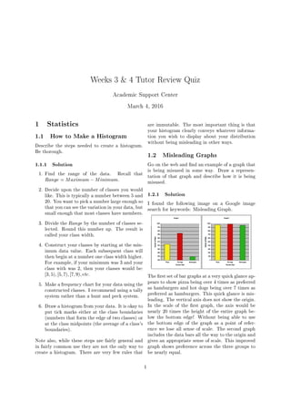
1.2 Misleading Graphs
Go on the web and
2. nd an example of a graph that
is being misused in some way. Draw a represen-
tation of that graph and describe how it is being
misused.
1.2.1 Solution
I found the following image on a Google image
search for keywords: Misleading Graph.
The
3. rst set of bar graphs at a very quick glance ap-
pears to show pizza being over 4 times as preferred
as hamburgers and hot dogs being over 7 times as
preferred as hamburgers. This quick glance is mis-
leading. The vertical axis does not show the origin.
In the scale of the
4. rst graph, the axis would be
nearly 20 times the height of the entire graph be-
low the bottom edge! Without being able to use
the bottom edge of the graph as a point of refer-
ence we lose all sense of scale. The second graph
includes the data bars all the way to the origin and
gives an appropriate sense of scale. This improved
graph shows preference across the three groups to
be nearly equal.
1
5. 1.3 What Eect Does Changing One
Data Point Have?
Suppose there are 100 people employed in a com-
pany. How will each of the following be aected if
the person with the highest salary gets a $10k raise
(be speci
6. c)? Why?
1. Median salary at the company
2. Mean salary at the company
3. Range of salary at the company
4. Interquartile range of salary at the company
1.3.1 Solution
1. The median salary is the middle data value on
a ranked listing. As only the maximum datum
is changed, no rankings change nor does the
location of the middle value. The median value
is unaected.
2. The mean salary depends on every data value.
As data values either stayed the same or went
up, we expect the mean to go up. Let xi be the
salary of the ith person in an ordered ranking.
Then we have
x =
x1 + x2 + : : : + x99 + x100
100
xnew =
x1 + x2 + : : : + x99 + x100 + 10000
100
xnew =
x1 + x2 + : : : + x99 + x100
100
+
10000
100
xnew = x + 100
Thus, the mean will go up by $100.
3. The range depends on the extreme data val-
ues. Since the maximum increases by $10000
we expect the range to increase by the same
amount. That is to say
range = max min
rangenew = max + 10000 min
rangenew = max min + 10000
rangenew = range + 10000
So, the range increased by 10000.
4. The IQR depends on the 1st quartile and the
3rd quartile. Neither of these are aected by
changing the maximum datum. Thus the IQR
is unaected.
1.4 Common Histogram Errors
Describe some of the common mistakes in making
histograms and how you might help people correct
them.
1.4.1 Solution
Often, people do not clearly label their classes.
Any histogram should clearly indicate whether
their horizontal axis ticks are for class mid-
points or for class boundaries. In either case, it
should also be indicated how data exactly on a
class boundary is assigned to each class (given
completely to the lesser class, completely to
the upper class, or split between them).
Histograms should not have spaces between
the class bars (unless one of the classes is
empty). That is, the horizontal axis is just as
important as the vertical axis in a histogram.
Histograms should always include the origins
of each axis when an absolute comparison of
values is relevant.
1.5 Pros and Cons of Various Mea-
sures of Location and Spread
Discuss the advantages and disadvantages of using
median vs mean vs mode for measures of the lo-
cation of a distribution. Do the same for IQR vs
standard deviation vs range for measures of spread
of a distribution.
1.5.1 Solution
Location. For unimodal symmetric distributions
all three of mean, median, and mode will roughly
coincide. For skewed distributions the mean will
typically be aected by more than the median.
Which is appropriate depends upon whether one
wishes to give equal weight to outliers or to focus
on the central portion of the data. Means have
the advantages of being easier to calculate for con-
tinuous distributions. Medians and modes tend to
be easier for discrete distributions (though the ad-
vent of computers makes computation of statistics
of discrete data sets somewhat of a non-issue most
of the time.)
Dispersion. The standard deviations tends to
2
7. have the same advantages that the mean does.
While the IQR and range tend to share advantages
with the median. There is no obvious analog to
modes for dispersion.
2 Trigonometry
2.1 Graphing Trigonometric Func-
tions
Sketch graphs of the following trigonometric func-
tions.
1. y = 3sin(4x ) + 1
2. y = sec(2x =3)
3. y = tan(2x =2)
2.1.1 Solution
1. The underlying graph for this problem is a sine
graph. We will use the concepts of amplitude,
period, phase shift, and vertical shift to mod-
ify the standard sine graph into this particular
graph.
Amplitude. The amplitude of a sine graph is
given by the absolute value of the coecient of
the sine function. In this case j3j = 3 and so
the amplitude is 3.
Period. The period of a sinusoidal graph
times the angular frequency will always equal
the period of the standard version of that
graph. The angular frequency, often called ! ,
is the coecient of x, in this case 4. Thus we
solve 4T = 2 and
8. nd that T, the period, is
=2.
Phase Shift. The phase shift is nothing more
or less than where the argument of the sinu-
soidal graph is 0. We set 4x = 0 and solve
for x to
9. nd x = =4 and so the phase shift
is =4. This is where our graph will begin
(that is, the behavior at 0 on a standard graph
is shifted to this value on our graph).
Vertical Shift. Any vertical shift will locate
the midline of our sinusoidal graph up or down
from the x-axis. Our vertical shift in this case
is 1, thus the graph will be moved up 1 to be
centered on the line y = 1.
We can begin by creating a graph with the cor-
rect midline. Then we can plot points every
1=4 of a period starting at our phase shift.
-2 p -
3 p
2
-p -
p
2
p
2
p
3 p
2
2 p
-3
-2
-1
1
2
3
4
5
Now we can connect our plot with a sinusoidal
curve and repeat it with the correct period.
-2 p -
3 p
2
-p -
p
2
p
2
p
3 p
2
2 p
-3
-2
-1
1
2
3
4
5
2. This next one is similar to the
10. rst except that
we cannot call our vertical stretch an ampli-
tude; however it is still found as j 1j = 1.
Our Period is 1. The phase shift is 1=6. There
is 0 vertical shift. So, starting with a basic
y = secx graph and modifying similarly we
get the following sequence as we build a graph.
-
4
3
-
13
12
-
5
6
-
7
12
-
1
3
1
6
5
12
2
3
11
12
7
6
17
12
-3
-2
-1
1
2
3
3. This one again follows the same pattern. There
is no vertical stretch factor. The period of a
standard tangent function is only instead of
2. Thus we instead solve !T = and
12. =4.
-p -
3 p
4
-
p
2
-
p
4
p
4
p
2
3 p
4
p
-3
-2
-1
1
2
3
2.2 Building a Trigonometric Func-
tion from Limited Data
Find a sinusoidal function with largest possible pe-
riod that has a local maximum at ( 2; 3) and a
local minimum at (4; 1).
2.2.1 Solution
A maximum and minimum of a sinusoidal trigono-
metric function will be at least 1=2 period apart.
Therefore, the maximum period will be twice this
gap. Our points have an x-separation of 6 so our
period will be 12. So, ! ¡ 12 = 2 gives ! = =6.
The average of the y-values of a maximum and
minimum will be the location of the midline and
hence the amount of our vertical shift, in this case
3 1
2
= 1. The amplitude is the distance between
the midline and an extrema, in this case 3 1 = 2.
Our phase shift will depend on what kind of si-
nusoidal function we wish to chose; any will work.
I will select a cosine function. At the beginning
of a period, cosine graphs start at their maxi-
mum. We know a maximum occurs at x = 2
and so we can select a phase shift of -2. Thus
x = 2 is a solution to =6x ' = 0 and so
' = =3. We then have the formula for our func-
tion: y = 2cos(=6x + =3) + 1.
2.3 Inverse Issues
For what values of x are the following formulae
true?
1. sin(arcsinx) = x
2. arcsin(sinx) = x
2.3.1 Solution
Arcsine and sine are inverses only upon restricting
the domain of our angle to be the principle domain,
which for sine is [
2
;
2
]. The corresponding sine
values range from -1 to 1.
1. Here, x represents a sine value, thus we must
have x P [ 1; 1].
2. Here, x represents an angle value, thus we must
have x P [
2
;
2
].
2.4 Evaluating Trigonometric Com-
positions
Evaluate the following.
1. cos(arcsin(7=6))
2. arctan(sin(3=2))
3. cos(arcsin(3=5))
2.4.1 Solution
Parts 1 3 can be done with diagrams on the unit
circle. Part 2 is most easily done with direct eval-
uation using memorized values.
1. We draw our standard position representation
of the angle 7
6
. This angle has a reference
angle of
6
. We (should) have the side lengths
for this reference triangle memorized. From
the picture we see cos 7
6
= p3
2
.
7 p
6
-
1
2
-
3
2
-1 1
-1
1
4
13. 2. sin 3
2
= 1 and so arctan(sin 3
2
) =
arctan( 1) =
4
.
3. arcsin(3=5) is a
16. ll in
the missing sides of our triangle. We can then
see cos(arcsin(3=5)) = 4=5.
sin-1
3
5
3
5
4
5
-1 1
-1
1
2.5 Establishing Identities
Establish the following identity.
sec
1 sin
=
1 + sin
cos3
2.5.1 Solution
This is an exercise in algebraic manipulation.
There are many possible routes that work. One
is shown below.
sec
1 sin
=
1 + sin
cos3
1 + sin
1 + sin
¡ sec
1 sin
=
sec(1 + sin)
1 sin2
=
sec ¡ 1 + sin
1 sin2
=
1
cos
¡ 1 + sin
cos2
=
1 + sin
cos3
=
1 + sin
cos3
X
3 Pre-calculus
3.1 Asymptotes of a Rational Func-
tion
Find all straight line asymptotes of y =
x3
+ x2
12
x2 4
.
3.1.1 Solution
Straight line asymptotes can come from two
sources: the end behavior (slant or horizontal
asymptote) or a vertical asymptote. We will in-
vestigate each separately.
Vertical Asymptotes. Vertical asymptotes of ra-
tional functions can be found by fully reducing the
ratio and examining where the remaining factors of
the denominator have roots.
y =
x3
+ x2
12
x2 4
y =
(x 2)(x2
+ 3x + 6)
(x 2)(x + 2)
y =
x2
+ 3x + 6
x + 2
; x T= 2
Thus we have a vertical asymptote when x+2 = 0,
that is, x = 2.
End Behavior. To
17. nd the long term behavior we
actually carry out the division in the de
18. nition of
y.
(x3
+ x2
12) ¤(x2
4) = x + 1 +
4
x + 2
Since 4
x+2
3 I as x 3 0 we see that y % x + 1 as
x 3 I. Thus y = x + 1 is a slant asymptote of y.
3.2 Solving an Inequality
Solve
x3
x
x 1
x3
3.2.1 Solution
This inequality is of the form f(x) g(x). We
can investigate such an inequality by rewriting it
5
19. as 0 g(x) f(x) and then making a sign chart.
x3
x
x 1
x3
0 x3
x3
x
x 1
0
x3
(x 1) (x3
x)
x 1
0
x3
(x 1) x(x2
1)
x 1
0
(x 1)(x3
x(x + 1))
x 1
0
(x 1)x(x2
x 1)
x 1
0
(x 1)x(x 1+
p5
2
)(x 1 p5
2
)
x 1
x ( I;
1 p5
2 ) ( 1 p5
2 ; 0) (0; 1) (1;
1+
p5
2 ) ( 1+
p5
2 ; I)
rhs + +
Thus we see the solution is (1 p5
2
; 0] ‘[1+
p5
2
; I).
3.3 Factoring a Polynomial
Factor 4x4
3x3
4x + 3.
3.3.1 Solution
We begin by using the rational root theorem to
20. nd
possible rational roots and hoping we have some.
The rational root theorem says if the polynomial in
question has only integer coecients (such as ours)
the only possible rational roots will be of the form
¦ a factor of the constant term
a factor of the leading coecient
In this problem, the factors of the constant are
f1; 3g and the factors of the leading coecient
are f1; 2; 4g thus our possible rational roots are
f¦1; ¦1
2
; ¦1
3
; ¦3; ¦3
2
; ¦3
4
g.
It is easiest to check for a root with synthetic divi-
sion (see the next problem). We start trying num-
bers.
4 -3 0 -4 3
1 4 1 1 -3
4 1 1 -3 0
Because the last digit was a 0 we see that 1 is a
root (we got lucky on the
21. rst try). Let's look for
more.
4 1 1 -3
1 1 2 3
4 2 4 0
1 is a root a second time. This illustrates the im-
portance of checking for multiple roots. At this
point we can factor our expression using two linear
factors and one quadratic.
4x4
3x3
4x + 3 = (x 1)2
(4x2
+ 2x + 3)
We could check 1 again, and then the remainder
of the possible roots, but none of them will end
up working (try one). However, we have other
techniques of
22. nding roots of a quadratic. The
quadratic formula is employed below to
23. nd them.
x =
2 ¦
p
22 4(4)(3)
2(4)
=
1 ¦i
p
11
4
And so the complete factorization of our polyno-
mial is
4x4
3x3
4x+3 = 4(x 1)2
(x 1 + i
p
11
4
)(x 1 i
p
11
4
)
Don't forget to have the leading 4.
3.4 Synthetic Division
Divide x4
6x3
12x + 2 by x 2 using synthetic
division.
3.4.1 Solution
This is simply a matter of recalling the operation
of synthetic division. Write the coecients of
the dividend in descending order making sure to
include 0's for any omitted orders. Write the root
of the divisor (which must be monic and linear)
outside. The pattern is to add the top entry to
the middle entry to get the bottom entry. Then
multiply that bottom entry by the root outside to
get the middle entry of the next column. The
24. rst
blank middle value is a 0.
1 -6 0 -12 2
2 2 -8 -16 -56
1 -4 -8 -28 -54
Now, the bottom row is the coecients of the quo-
tient in descending order, and the last is the coef-
25. cient of the remainder. 1 -4 -8 -28 -54
corresponds to x3
4x2
8x 28 54
x 2
. This is
the result of the division.
6
26. 3.5 Finding Graphing an Inverse
Find the inverse of f(x) = e3x+2
1. Sketch both
f and f 1
on the same set of axes.
3.5.1 Solution
To
27. nd an inverse we substitute f(x) 3 x and x 3
f 1
(x) then solve the result for f 1
(x).
f(x) = e3x+2
1
x = e3f 1
(x)+2
1
x + 1 = e3f 1
(x)+2
ln(x + 1) = 3f 1
(x) + 2
ln(x + 1) 2
3
= f 1
(x)
Below is a simultaneous plot of both functions. The
original function is on top, the inverse is on bottom,
and the dotted line is just to emphasize the re
ec-
tion nature that inverses will always have.
-4 -2 2 4
-4
-2
2
4
4 Calculus I
4.1 Possible Properties of Functions
True or false:
1. If f(x) M has a non-empty solution set no
matter how big M is then limx3I f(x) = I
2. A function cannot have two horizontal asymp-
totes.
3. Functions cannot cross their asymptotes.
4.1.1 Solution
1. False. The stated condition says that a graph
of f would go above the line y = M at least
once no matter how big M is. However, going
above a line is not equivalent to staying above
that line. For example, y = x sinx will eventu-
ally be as large as we wish, however, it also re-
visits 0 twice within any interval of length 2.
The function wiggles back and forth with ever
increasing amplitude. Such a function cannot
have any limit, even an in
28. nite one.
2. False. A horizontal asymptote is a horizontal
line that the graph approaches in either direc-
tion. Since we have two directions to travel,
left and right, we can have two dierent hori-
zontal asymptotes. y = tan 1
x is such a func-
tion, its two asymptotes being y = ¦
2
.
3. False. There is no requirement whatsoever for
functions to not cross their asymptotes. y =
sin x
x is a function that crosses its asymptote,
y = 0, in
29. nitely many times.
4.2 Mutual Tangent Lines
There are exactly 2 lines tangent to both y = x2
y = 1 (x 2)2
. Find equations for those lines.
[Bonus Challenge: Can you solve this again without
using calculus?]
4.2.1 Solution (Calculus)
A picture of the situation is immensely helpful.
-2 -1 1 2 3 4
-2
-1
1
2
3
4
Hx2,y2L
Hx1,y1L
Hx2,y2L
Hx1,y1L
7
30. Here we can see the two lines. They are each de-
termined by a pair of points at which the lines are
tangent to the two curves respectively. We will
31. nd
conditions for the four variables: x1; y1; x2; and y2.
The point (x1; y1) must be on the curve y = x2
.
Thus,
y1 = x2
1
Similarly, the point (x2; y2) must be on the
curve y = 1 (x 2)2
and so
y2 = 1 (x2 2)2
The slope of the line must be the slope of the
curve y = x2
at the point (x1; y1) thus
y2 y1
x2 x1
= 2x1
Also, the slope of the line must be the slope of
the curve y = 1 (x 2)2
at the point (x2; y2)
so
y2 y1
x2 x1
= 2(x2 2)
This is four equations with four unknowns. We
will solve this as a system of equations.
y1=x2
1
These are our
initial equations.
y2=1 (x2 2)2
y2 y1
x2 x1
=2x1
y2 y1
x2 x1
= 2(x2 2)
1 (x2 2)2
x2
1
x2 x1
=2x1
Substitute the y's
out using the
32. rst
two equations.1 (x2 2)2
x2
1
x2 x1
= 2(x2 2)
1 (x2 2)2
(x2 2)2
x2 (x2 2)
= 2(x2 2) Subtract one equa-
tion from the other
to obtain x1 = 2
x2 then substitute
into the top equa-
tion.
x2=2¦p2
2
Solve for x2
1st Solution 2nd Solution
x1=2+
p2
2
x1=2 p2
2
x2=2 p2
2
x2=2+
p2
2
y1=3+2
p2
2
y1=3 2
p2
2
y2= 1 2
p2
2
y2= 1+2
p2
2
Back substitute
each solution
(separately) to
obtain the two
solutions.
Now we can
33. nd the equation of the line that goes
through each pair of points. It is convenient to
note that the slope of the line is equal to 2x1 by
our original equations.
y = (2 +
p
2)(x 2 +
p
2
2
) +
3 + 2
p
2
2
y = (2
p
2)(x 2
p
2
2
) +
3 2
p
2
2
With a little eort we can rearrange these as
y = (2 +
p
2)(x 1) +
1
2
y = (2
p
2)(x 1) +
1
2
These are the two lines.
8
34. 4.2.2 Solution (Algebra)
In this very dierent approach to the problem, we
make use of two observations:
The two lines intersect at one point. If we can
35. nd that point directly we will be half way
done.
The only lines that intersect a parabola exactly
once are lines tangent to the parabola or par-
allel to the parabola's line of symmetry (which
in this case is vertical and not a possibility).
We begin by
36. nding the point of intersection of
the two lines. The point of intersection is a point
of rotational symmetry of the combined graph of
the two parabolas. That is, if we rotate the two
parabolas 180 around the point of intersection we
get the same image. The below diagram will help
illustrate this.
-2-1 1 2 3 4
-2
-1
1
2
3
4
-2-1 1 2 3 4
-2
-1
1
2
3
4
-2-1 1 2 3 4
-2
-1
1
2
3
4
-2-1 1 2 3 4
-2
-1
1
2
3
4
-2-1 1 2 3 4
-2
-1
1
2
3
4
This means that any line connecting corresponding
points will rotate into itself. The line connecting
the verticies is such a line and thus the midpoint
of the line segment containing the two verticies
must be the point of intersection.
The two verticies are (0; 0) and (2; 1) the midpoint
of the segment connecting these two points is (1; 1
2
)
and this must be our common point of intersection
of the sought lines.
To
37. nd the appropriate slopes we try a very
dierent approach. It is generally true that any
curve which is either always concave up or always
concave down will intersect its own tangent lines
exactly once (at the point of tangency). We will
38. nd all such lines that go through our earlier
de
39. ned common point. Let y = m(x 1) + 1
2
be
our sought line. We wish for this to intersect with
our curves (we will concentrate upon y = x2
for
simplicity) exactly one time.
y = m(x 1) +
1
2
y = x2
x2
= m(x 1) +
1
2
0 = x2
mx + m 1
2
This quadratic equation has discriminate
m2
4(m 1
2
). A quadratic equation has a
unique solution exactly when its discriminate is 0.
m2
4m + 2 = 0
(m 2)2
2 = 0
jm 2j =
p
2
m = 2 ¦
p
2
Thus the only two possible slopes are 2 +
p
2 and
2
p
2. Since we know there are indeed two such
lines, they must have these slops. This yields the
lines
y = (2 +
p
2)(x 1) +
1
2
y = (2
p
2)(x 1) +
1
2
Which are, of course, the same as we got from the
calculus method.
4.3 Dierentiating Using the De
41. nition of the derivative to dierentiate
the following functions.
1. f(x) = x3
x
2. g(x) =
1
(x 2)2
3. h(x) =
p
x2 4
9
42. 4.3.1 Solution
No fancy tricks on this one, just some direct evalu-
ation of limits.
1.
fH(x) = lim
h30
f(x + h) f(x)
h
fH(x) = lim
h30
(x + h)3
(x + h) (x3
x)
h
fH(x) = lim
h30
3x2
h + 3xh2
+ h3
h
h
fH(x) = lim
h30
(3x2
+ 3xh + h2
1)
fH(x) = 3x2
1
2.
fH(x) = lim
h30
f(x + h) f(x)
h
fH(x) = lim
h30
1
(x+h 2)2 1
(x 2)2
h
fH(x) = lim
h30
(x 2)2
(x+h 2)2
(x+h 2)2(x 2)2
h
fH(x) = lim
h30
2xh 4h + h2
h(x + h 2)2(x 2)2
fH(x) = lim
h30
2x 4 + h
(x + h 2)2(x 2)2
fH(x) =
2x 4
(x 2)4
fH(x) =
2
(x 2)3
3.
fH(x) = lim
h30
f(x + h) f(x)
h
fH(x) = lim
h30
p
(x + h)2 4
p
x2 4
h
fH(x) = lim
h30
(x + h)2
4 (x2
4)
h(
p
(x + h)2 4 +
p
x2 4)
fH(x) = lim
h30
2xh + h2
h(
p
(x + h)2 4 +
p
x2 4)
fH(x) = lim
h30
2x + h
p
(x + h)2 4 +
p
x2 4
fH(x) =
x
p
x2 4
4.4 Finding Example Functions
Find speci
43. c examples of the following.
1. A function that has a tangent line at every
point on its graph but is not dierentiable on
all of R.
2. A function with f(x) 0 fH(x) 0 for every
x in R.
3. A bounded function with fH(x) 0 for every
x in R.
4.4.1 Solution
1. First, note that not dierentiable on all of R
means that there is at least one point where
it fails to be dierentiable. It does not say
that the function is not dierentiable at every
point of R. There is only one way a function
can fail to be dierentiable, but still have a
tangent line at a particular point, the case of a
vertical tangent. Any function with a vertical
tangent line at a particular point will suce.
f(x) = x
1
3 is such a function with the interest-
ing location at the origin.
2. f(x) 0 means f is above the x-axis and
fH(x) 0 means f is decreasing. So we want
a function that is always decreasing but never
touches or goes below the x-axis. There are
many such functions. f(x) = e x is one such
example. So is f(x) = tan 1
x +
2
.
10
44. 3. fH(x) 0 means f is increasing. We want
a function that is bounded (trapped between
two values) but is always increasing. Again,
there are many examples. f(x) = tan 1
x is
one such example.
4.5 Another Derivative Via the Def-
inition
Find d
dx sinx via the de
45. nition.
4.5.1 Solution
Again, we will use no special tricks and just break
apart the limit into pieces we know.
d
dx
sinx = lim
h30
sin(x + h) sinx
h
d
dx
sinx = lim
h30
sinx cosh + cosx sinh sinx
h
d
dx
sinx = lim
h30
cosx sinh
h
+
sinx(cosh 1)
h
d
dx
sinx = cosx ¡1 + sinx ¡0
d
dx
sinx = cosx
5 Calculus II
5.1 Evaluating an Inde
46. nite Integral
Evaluate
‚ 1px2 2xdx.
5.1.1 Solution
This is a challenging Calculus II integral. We will
make use of hyperbolic trigonometric functions to
evaluate this integral. Here are a few relevant facts
about hyperbolic trigonometric functions.
De
47. nitions
coshx =
ex + e x
2
sinhx =
ex e x
2
Some Formulas
d
dx coshx = sinhx
d
dx sinhx = coshx
cosh2
x sinh2
x = 1
Graphs
-3 -2 -1 1 2 3
-3
-2
-1
1
2
3
cosh x
sinh x
Inverses If x ! 0 then we can invert coshx as
y = coshx
y =
ex + e x
2
0 = ex 2y + e x
0 = (ex)2
2yex + 1
ex =
2y ¦
p
4y2 4
2
ex = y ¦
p
y2 1
x = ln
y ¦
p
y2 1
We chose the + branch for the principle inverse
hyperbolic cosine.
y = sinhx
y =
ex e x
2
0 = ex 2y e x
0 = (ex)2
2yex 1
ex =
2y ¦
p
4y2 + 4
2
ex = y +
p
y2 + 1
x = ln
y +
p
y2 + 1
Here we are forced to chose the + branch if we
want a real inverse so that the exponential in
the second to last line is positive.
11
48. Okay, time for the integral.
1
p
x2 2x
dx =
1
p
(x 1)2 1
dx
=
1
p
(u)2 1
du
Here we wish to make the substitution u = cosht
so that we can make use of the hyperbolic trigono-
metric identity and simplify the radical in the de-
nominator. Unfortunately, to do so we need pay
attention to the sign of u.
u 1 1 u
Let t ! 0
u = cosht u = coshtdt
du = sinht du = sinhtdt
‚ sinhtdt
p
( cosht)2 1
‚ sinhtdt
p
(cosht)2 1
Then, because cosh2
t 1 = sinh2
t
‚ sinhtdt
p
sinh2
t
‚ sinhtdt
p
sinh2
t
And since sinht ! 0 for t ! 0
‚ sinhtdt
sinht
‚ sinhtdt
sinht
‚
dt
‚
dt
t + c1 t + c2
cosh 1
u + c1 cosh 1
u + c2
ln
u +
p
u2 1
¡
+ c1 ln
u +
p
u2 1
¡
+ c2
At this point, we back substitute u = x 1 and
obtain
1
p
x2 2x
dx
=
V
`
X
ln
x + 1 +
p
(x 1)2 1
+ c1; x 2
ln
x 1 +
p
(x 1)2 1
+ c2; x 2
5.2 What is a Dierential Equation?
What is a dierential equation? What does solving
a dierential equation mean?
5.2.1 Solution
A dierential equation is a relation between a func-
tion and its own derivative(s).
A solution to a dierential equation is a function
de
49. ned on a set containing an open interval that
satis
50. es the given dierential equation at all points
in its domain.
5.3 Using a Slope Field
Plot a slope
51. eld for dy
dx = x+1
y 2
. Overlay several
typical solution curves. Without solving the equa-
tion guess the general solution. Check this using
implicit dierentiation.
5.3.1 Solution
The most direct way to plot a slope
52. eld is to gener-
ate a grid of (x; y) points and evaluate the slope at
each point, plotting it as a small segment with that
slope at the grid point used. For example, in this
problem, chosing a grid point of (2; 1) would yield
a slope of dy
dx = 2+1
1 2
= 1 and so at the point (2; 1)
we would draw a small segment of slope 1. Doing
this for many grid points will generate a picture like
below left.
-4 -2 0 2 4
-4
-2
0
2
4
-4 -2 0 2 4
-4
-2
0
2
4
We can now sketch in several typical solution curves
by selecting an initial condition and then drawing a
path that is tangent to the slope
53. eld at all points
along the curve, as above right.
We sketched circles. It would be dicult to deter-
mine with certainty from a slope
54. eld alone if the
true solutions are exactly circles, or indeed even
closed curves. However, we can check if this is the
12
55. case easily because we have the original dierential
equation. Checking is simply a matter if seeing if
this family of concentric circles satis
56. es the dier-
ential equation.
Our circles appear to be centered at (1; 2) and so
the family can be described as
(x 1)2
+ (y 2)2
= r2
r 0
Dierentiating implicitly and solving for dy
dx we get
2(x 1) + 2(y 2)
dy
dx
= 0
dy
dx
=
x + 1
y 2
Thus our family of curves do solve the dierential
equation.
5.4 Mixing Problem
A vat holds 20 gal of pure water. At time t = 0 we
begin pumping in a .3 kg/gal solution of brine at
a rate of 6 gal/min. The solution is thoroughly
mixed and continuously drained at a rate of 3
gal/min. What volume of solution will be in the
tank when the concentration of the solution is .2
kg/gal (assume the tank is as large as necessary for
no spilling)?
5.4.1 Solution
Mixing problems can be attacked by setting up a
model in the form of a dierential equation. We
will do so. [Note, I have chosen to keep units
throughout the entire computation. This make it
somewhat messier. It is not necessary to do so,
but I wished to exhibit that you can do it if you
want/need to].
Let S(t) = the mass of salt in the tank at
time t. Then the law of conservation of mass says
dS
dt
= hsalt coming ini hsalt going outi
We can then model the
ow of salt in or out of the
tank as the concentration of solution
owing times
the rate of
ow. For us,
dS
dt
=
:3kg
gal
6gal
min
hconcentration in tanki 3gal
min
Unfortunately, we do not know the concentration
in the tank, but we can write an expression for it
involing S.
dS
dt
=
:3kg
gal
6gal
min
S
hvolume in tanki
3gal
min
Because we start with 20gal of solution and we are
pumping in 3gal more per minute than we take out,
our volume of solution as a function of time must
be expressed by 20gal + 3gal
mint. Upon substitution
we have
dS
dt
=
:3kg
gal
6gal
min
S
20gal + 3gal
mint
3gal
min
dS
dt
=
1:8kg
min
3S
20min + 3t
This is a linear dierential equation. We solve it as
such (assume 20 + 3 t
min 0).
dS
dt
+
3
20min + 3t
S =
1:8kg
min
(t) = e
R 3
20min+3t
dt = e
R du
u = u = 20min + 3t
(20min + 3t)
dS
dt
+ 3S =
1:8kg
min
(20min + 3t)
d
dt
[(20min + 3t)S] = 36kg + 5:4kg
t
min
d
dt
[(20min + 3t)S]dt =
36kg + 5:4kg
t
min
dt
(20min + 3t)S = 36kg t + 2:7kg
t2
min
+ C
S =
36kg t + 2:7kg t2
min + C
20min + 3t
Because S(0) = 0 (the tank holds only pure water
at the begining) we must have C = 0.
S =
36kg t + 2:7kg t2
min
20min + 3t
S =
36 t
min + 2:7( t
min)2
20 + 3 t
min
kg
13
57. The concentration in the tank is then
S
volume in tank.
:2
kg
gal
=
36 t
min + 2:7( t
min)2
20 + 3 t
min
kg
¤
20gal +
3gal
min
t
:2 =
36 t
min + 2:7( t
min)2
(20 + 3 t
min)2
:2(20 + 3
t
min
)2
= 36
t
min
+ 2:7(
t
min
)2
0 = 4:5(
t
min
)2
+ 60
t
min
400
And so, t = 18:2137min or t = 4:88034min.
Clearly we chose the positive time since a negative
time makes no sense in this problem.
5.5 Euler's Method
Use Euler's Method with a step size of 1
4
to approx-
imate the value of y(1) if yH = x2
+ y2
y(0) = 0.
5.5.1 Solution
Euler's method gives us a way to approximate y(x)
given an initial condition (x0; y0) and a dierential
equation dy
dx = f(x; y). It works by following the
slope