dff fvfvdfv fdvdfvdfv dfvdfvdfvdfv

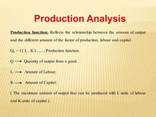
1. Production Analysis
Production function: Reflects the relationship between the amount of output
and the different amount of the factor of production, labour and capital.
Qx = f ( L , K ) …… Production function.
Q Quantity of output from x good.
L Amount of Labour.
K Amount of Capital.
( The maximum amount of output that can be produced with L units of labour
and K units of capital ).

2. Production function
Short Term Long Term
Reflects the relationship All factors of production will
between Q and Labour with change.
fixed amount of capital. Reflects the relationship between
Q = F ( L , K ). the size of the firm and the
quantity of output.
Q = F ( L , K ).

3. Short Term: what is the relationship between the amount of output from good
x when the amount of labour changes with fixed amount of capital? This
relationship is controlled by increasing and diminishing return Law.
Long Term: what is the relationship between the amount of output from
good x when the amount of both labour and capital change?? This
relationship is controlled by Returns to Scale Law.

4. PRODUCTION FUNCTION FORMS
1- Linear Production function:labour and capital are perfect substitutes.
Q = F ( L , K ) = aL+ bk
2- Leontief Production function: labour and capital are used in fixed
proportions.
Q = F ( L , K ) = min (aL, bk )
3- Cobb – Douglas Production function: labour and capital have a degree
of substitutability.
Q = F ( L , K ) = La
K
b
a and b are constant, L amount of labour and K amount of capital.

5. IN GENERAL THE PRODUCTION FUNCTION:
 The maximum output that can be produced for a given amount of the
inputs ( L, K).
 The minimum amount of the inputs ( L , K) is necessary to produce a
given amount ofthe output.

6. PRODUCTION FUNCTION IN THE SHORT RUN
what is the relationship between the output from x good and the
different amount of labour with fixed amount of capital.
Suppose the relationship between the totaloutput of x good
and the amount of labour of capital, is represented in table (1). Based
on these data and information determines.
 Graphically the relationship between Q and L ?
 Determine the marginal and average productivity of labour
(numerically and graphically)?

7. PRODUCTIVITY LEVEL
The firm productivity by can be measured at two level of the
productivity.
 Marginal Productivity for each factor of production.
 Average productivity for each factor of production.
 Marginal productivity for labour ( MPL), measures the productivity
of last unit of labour (worker).
MPL=
∆𝑸
∆𝑳
= 𝒅𝑸𝟏
𝒅𝑳
= 𝝏𝑸𝟏
𝝏𝑳

8. Reflects the changes of the output as a result of changing of labour
by one unit ( worker ).
With the way you can determine the marginal productivity of capital
but if the capital is variable not fixed.
Average Productivity of labour ( APL ), measures the productivity of
each unit of labour ( worker ).
MPL =
𝑄
𝐿

9. AVERAGE PRODUCTIVITY FOR LABOUR
 First stage: increases with increasing of the number of workers to
reach the maximum value equals the MPL. At this stage note the
value ofAPLless MPLatalllevels ofworkers.
 Secondstage (diminishing Relurn)
Any increasing ofworkers more than 5 workers, leads to decreasing
ofAPLand more than 5 workers,the APLwillbe greaterthanMPL.

10. APL
220
APL
1 2 3 4 5 6 7 8 9 10 11Q
Explain the relationship between total output and both MPL, APL graphically?
Increase
Decrease

11. Based on the previous example these relationships could be represented in
graph (3)
First stage second stage third stage
Labor
1 2 3 4 5 6 7 8 9 10 11
880
330
Q
APL
MPL
Q
APL
MPL
220

12. Table (1)
L 1 2 3 4 5 6 7 8 9 10 11
K 10 10 10 10 10 10 10 10 10 10 10
Q 100 250 500 880 1100 1200 1250 1250 1100 1000 900
MPL 100 150 250
330 220 100 50 0 -150 -100 -100
APL 100 125 166.7 220
220 200 178.6 156.3 122.2 100 81.9

13. NOTE:
First stage: ( Increasing return )
 Total output increases with increasing rate ( the increasing of the
total output is called MPL ) with increasing of the labournumber.
 MPL increases with the increasing of labour, and will be greater than
average productivity at any level of workers.
 APL increases with any increasing of labour units and will be less
than MPL at any level of labour units.

14. SECOND STAGE:( DIMINISHING RETURN )
 Total output increasing with decreasing rate with any increasing of
labour.
 MPL decreasing with any increasing of labour units, to reach zero
value at unit (8) of labour. Through this stage after certain point will be
less than APL.
 APL still increases at the beginning of this stage with increases of
workers, to reach the maximum value at 5 workers any increasing of
labour units, the APL will decrease.

15. THIRD STAGE: (NEGATIVE RETURN – MPL
NEGATIVE )
 Total output decreases with any increasing of workers, adding any
workers not only doesn’t add any productivity but also will affect
negatively on the product of other workers.
 MPLwill be negative value with any increasing of labour.
 An APL continuum’s to decrease with any increasing of workers but
doesn’t be zero or negative values.

16. LONG TERM PRODUCTION FUNCTION
Inthelongtermtherechancetothefirmforchoosingthebestand
theoptimalcombinationsoflabourandcapital.Inothermeaningthereis
achancetotheoptimalsizeofthefirm.
To determine the optimal technical methods that could maximize
output andminimizecost,studyingbothISOcostarerequired.

17. ISO QUANT
- Is quant reflects the different combinations of labour and capital
(both of them are variable) that generate the same amount of
output. Graphically the ISO quant curve reflects the different
combinations of L & K that generate the same amount of
output.
- In general ISO represents the producers desire to produce.
- Through production functions, the ISO quant map can be
derived as represented in figure (1).

18. k 400
300 ISO quant map
200
100
4
3
2
1
L

19. FROM FIGURE (1):
- The movement from down to up on the ISO quant map reflects
more output and from up to down less output with a degree of
substitutionbetween L, K.
- The slope of ISO quant curve equals the marginal technical rate
of substitution “MTRS”, this slope decreases from up to down
on the same curve, for this reason the ISO quant curve is
concave to the origin point.
(MTRS)L,K =
∆𝐊
∆𝐋
(1)

20. LEONTIF PRODUCTION FUNCTION (ISO QUANT)
Q = f ( L, K ) = mini ( al, bk).
Where L, K are complementary factors of production, it means L, K will
change with fixed ratio as represented in figure (2).
K
300
200
100
3
2
1
L
Leontief ISO quant

21. WHICH THE OPTIMAL COMBINATION BETWEEN L, K,
THAT MAXIMIZE THE OUTPUT?
To determine the optimal combination of L and K, there are some
requirements:
- DetermineISOquantasisrepresentedbefore.
- DetermineISOcostasisexplainedinthefollowing:

22. ISO COST
ISOcostdependson,thepriceofinputs(L,K)andthefinancial
resourcesaredevotedtopurchaseinputs.Theproducerbudget(C)will
distribute between land K. the constraint budget, based upon the price
oflabour(W) andthepriceofcapital(i)where:
C=WxL+IK (2)

23. Where C refers to the total budget (cost), L refers to the number of
workers and K refers to the amount of capital, W and I refer to the price
of labour and capital respectively.
Suppose: labour and capital are purchased from perfect
competition mark, under this assumption W andI will be constant.
The budget line forproducer can be represented in figure (3).

24. What are the factors could affect on the ISO cost.
K
3 1 2
L

25. CHANGES OF THE FINANCIAL RESOURCES
 Other things being equal the increasing of the amount of
the financial resources leads to shift of the ISO cost up from
(1) (2) but the decreasing of the financial
resources shifts the ISO cost down from


26. CHANGES OF THE RELATIVE PRICE OF L AND K
Suppose the price of labour (W) increases, other things being equals,
the ISO cost rotates to the left from (1) (2), but the
decreasing of the price of labour rotates the ISO cost to the right from
(1) (3), figure (4).
K
2 1 3
L
ISO cost

27. OPTIMAL COMBINATION (L, K)
TheoptimalcombinationofLandKwillsatisfywhentheoutputis
atthemaximumlevelwithcertainamountofthefinancialresourcesasis
representedinfigure(5).

28. K
N
K1 E1 300
200
100
L1 M L
At E, where the budget line MN tangent with the ISO quant number (2),
at this point any movement on the ISO cost, achieves less output, only
at this point at this point the output will be at the maximum level.

29. EQUILIBRIUM CONDITION
-ISO cost tangents ISO quant.
-The slope of ISO cost equals the slope of ISO quant
𝑤
𝑙
=
MTRS
The optimal combination E, where the amount of labour L, and the
amount of K is K1 .

30. EXTENSION OF THE FIRM SIZE
Suppose the firm size increase as a result of increasing the
financial resources, the ISO cost will shift up as represented in figure (6).
The extension of the firm size will take one of the three paths:
- Extansion of the firm size with intensive of labour in the
production process (7-1).
- Extension of the firm size with capital intensive in the
production process (7-2).
- Extension of the firm size with neutraluses of labour and capital
(7-3).

31. (7-3) (7-2) (7-1)
E- Path E- Path
E- Path
K
L L L
K K