This report entails a project similar to Google's Page Rank algorithm.

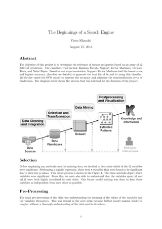
1. The Beginnings of a Search Engine
Viren Khandal
August 15, 2018
Abstract
The objective of this project is to determine the relevance of various url queries based on an array of 12
different predictors. The classifiers tried include Random Forests, Support Vector Machines, Decision
Trees, and Naive Bayes. Based on our experimentation, Support Vector Machines had the lowest error
and highest accuracy, therefore we decided to generate the text file of 0s and 1s using this classifier.
We further tuned the SVM model to increase the accuracy and minimize the misclassification error of
predictions. The diagram below shows the process that was followed for the duration of the project.
Selection
Before employing any methods onto the training data, we decided to determine which of the 12 variables
were significant. Performing a logistic regression, there were 8 variables that were found to be significant
due to their low p-values. This entire process is shown in the Figure 1. The three asterisks depict which
variables were significant. From this, we were also able to understand that the variables query id and
url id were both highly correlated to each other. Our future model making was done to keep these
variables as independent from each other as possible.
Pre-Processing
The main pre-processing of this data was understanding the meaning of the values of the variables and
the variables themselves. This was crucial in the next steps because further model making would be
tougher without a thorough understanding of the data and its structure.
1

2. Transforming the Data
The main transforming of the data was done using k-fold cross validation. We were able to set up an
environment, in which we ran 10-fold cross validation. This cross validation helped us verify that all of
our classifiers were working properly and were trained enough to perform well on the test set.
Data Mining
The majority of the project took place in this stage. We tested the performance of 4 different methods
and then decided which method to employ on the test data. The 4 methods we chose included Support
Vector Machines, Random Forests, Decision Trees, and Naive Bayes. The results of the 4 classifiers are
shown in the sub sections below.. As Support Vector Machines had the lowest error, we decided to move
on with this method and further tune it to decrease the error and maximize the accuracy of our model.
1. Decision Trees
The decision tree model that we built had an accuracy of approximately 61.5%. This was a significantly
low accuracy, therefore we had low hopes for the future tuning we would perform for decision trees. Yet,
we still went ahead with our tuning in the two methods shown below.
a. Tuning: Omitting Variables
To tune the parameters in the decision tree model from before, we decided to omit variables one at a
time. This helped us determine which variables had a significant impact to the outcome. The table
below shows several trials of variables that were left out against the accuracy of the model.
Omitted Variable Accuracy Misclassification Error
None Omitted 61.05% 38.95%
query id 61.6% 38.4%
url id 61.34% 38.66%
query length 62.02% 37.98%
is homepage 60.93% 39.07%
sig1 61.3% 38.7%
sig2 61.88% 38.12%
sig3 62.1% 37.9%
sig4 62.01% 37.98%
sig5 61.14% 38.86
sig6 60.9% 39.1%
sig7 61.75% 38.25%
sig8 61.25% 38.75%
b. Tuning: Pruning
To further test the effectiveness of the decision tree model, we decided to use pruning to remove the
unnecessary elements of the decision tree. This gave us much more accurate results and provided us
an accuracy value of approximately 64%. Although this was not very close to the accuracy of Random
Forests or SVM, it was worthwhile to understand how pruning works on the training dataset.
2. Naive Bayes
The results from the Naive Bayes model are shown in Figure 2. The overall accuracy came to be around
60%. This was a very low value compared to our various other models. We tried to implement an
lplace smoothing metric on our Naive Bayes model, however, it did not result in a significant increase
in accuracy. Due to this and the limited time, we decided not to go further with Naive Bayes and not
further tune the model.
2

3. 3. Random Forest
The main results from running Random Forests are shown in the figures at the end. The error, using a
validation set for predictions, came to be around 34%. To further analyze the causes of the error and
in hopes to increase accuracy, we tuned the random forest by removing the less important predictors
(found from logistic regression). This tuning, however, did not have a significant impact on decreasing
the error.
a. Tuning: Changing Number of Trees
The table below shows how accuracy changed based on the number of trees inputted to our Random
Forest model. As you can see, there is a gradually increasing pattern, however, the accuracy is not
significantly changing.
Number of Trees in Model Accuracy Misclassification Error
100 65.2% 34.8%
500 65.6% 34.4%
1000 66.1% 33.9%
2000 66.4% 33.6%
b. Tuning: Omitting Variables
The next form of tuning we tried for our Random Forest model was omitting one variable from the
model and calculating the accuracy. The table below shows the results of the omitting trials. Although
there is a higher accuracy in some models than others, SVM was an overall better model, due to its high
accuracy rate. Therefore, we decided to move on to tuning our last classifier: Support Vector Machines.
Omitted Variable Accuracy Misclassification Error
None Omitted 66.1% 33.9%
query id 65.92% 34.08%
url id 65.93% 34.07%
query length 65.1% 34.9%
is homepage 65.86% 34.14%
sig1 65.65% 34.35%
sig2 64.03% 35.97%
sig3 64.54% 35.46%
sig4 65.12% 34.88%
sig5 65.34% 34.66%
sig6 64.87% 35.13%
sig7 64.73% 35.27%
sig8 65.34% 34.66%
4. Support Vector Machine
SVM turned out to have the highest accuracy, 67%, out of all of our models. Although it had an accuracy
very close to that of Random Forest, we decided to move on with tuning our SVM to reduce the error.
The two main ways we tuned our model were using different types of kernels and changing the cost for
each model.
a. Tuning: Changing Kernels
We began our testing with a linear kernel model. This model constantly gave an accuracy of about 67%,
therefore we decided to try out polynomial kernel SVM. This method did not increase the accuracy, but
rather decreased by a few percentages. This immediate drop in accuracy alerted us to try radial based
kernel, which increased our accuracy to the highest it ever was, 67.8%. From these positive results of
the radial kernel SVM, we decided to move on by tuning this radial model through changing the cost of
each model.
3

4. Kernel Type with Cost of 1 Accuracy Misclassification Error
Linear 67.34% 32.66%
Polynomial 65.76% 34.24%
Radial 67.8% 32.2%
b. Tuning: Changing Cost
After determining that radial kernel SVM was the best model for our training data, we decided to tune
the model even more by changing the cost. We started off by putting the cost very low and gradually
increasing it. At the start, with the default cost of 1, the model had an accuracy of about 67.8%. We
continued to increase the cost until we reached 263. At this 263 cost value, we achieved a 69% accuracy
for our predictions. We continued to slowly add the cost, in an effort to decrease the error even more.
However, the accuracy continually decreased. We reverted back to our 263 cost radial kernel model and
created our text file of relevance predictions.
Cost Value with Radial Kernel Accuracy Misclassification Error
1 67.8% 32.2%
50 67.94% 32.06%
100 68.2% 31.8%
263 68.8% 31.2%
300 68.3% 31.7%
Evaluation
After creating the four models mentioned above, the following table was formed.
Model Type Max. Accuracy Misclassification Error
Decision Trees 64.05% 35.95%
Naive Bayes 60.14% 39.86%
Random Forest 66.4% 33.6%
SVM 68.8% 31.2%
This table shows that SVM had the highest accuracy value and would be the most effective in predicting
relevance correctly for the test data set. The tuning done to the original SVM model brought the
accuracy to a maximum of around 68.8%.
Note: The next three pages display several images and graphs that are referred to in the
body of this document.
4

5. Figure 1: This screen shot shows the logistic regression for the training data. This was used to figure
out which of the 12 predictors were significant and will be most important in the classifiers. The three
asterisks show which of the 12 different variables were most important, which is based on the p-value.
5

6. Figure 2: This is the resulting matrix of the Naive Bayes method. This can be used to calculate the
accuracy values mentioned in the document above
Figure 3: This image shows the confusion matrix and accuracy results for the Random Forest model. As
you can see, the accuracy is approximately 66%, therefore it is not as good as the final SVM model.
6

7. 0 500 1000 1500 2000
0.200.250.300.350.400.450.50
rf1
trees
Error
Figure 4: This graph displays the errors of the Random Forest model from Fiure 3. The middle black
line is the most important line to us, as it is the misclassification error. As seen in the image, the
misclassification error never seems to decrease much below 34%.
7