1. Nguyen 1
John Nguyen
1373244
Nonexperimental Datasets: Can We Utilize Them To Cut Testing Costs?
1. Abstract
In this paper, we are answering the question whether we can replicate results found using
the experimental dataset with a nonexperimental dataset that uses the Panel Study of Income
Dynamics as a source for the comparison group. We also lightly touch on the change in
estimated earnings due to the job training program. While we are able to trust the experimental
regression estimate when observables are added, the nonexperimental regression estimate shows
signs of bias, created from the Panel Study of Income Dynamics comparison group. We can
conclude a regression cannot fix a bias of this magnitude because the addition of observables to
the basic bivariate OLS regression is unable to fully reduce the bias. This issue derives from our
nonexperimental control group being chosen, allowing both a selection and omitted variable bias
to occur. Only a counterfactual that is randomly chosen or an obscene amount of covariates can
solve the issue.
2. Introduction
The goal of this paper is to determine if the results found from the experimental dataset
can be replicated by a nonexperimental that contains the Panel Study of Income Dynamics as its
comparison group. If the results can be replicated, economists should consider transitioning from
2. Nguyen 2
using a randomly assigned control group to a control group comprised of participants in the
Panel Study of Income Dynamics.
Two major regressions occurred: one with an experimental dataset and one with a
nonexperimental. These dataset only differ in the composition of the control groups. The
experimental control group is randomly assigned to the group while the nonexperimental is
selected from the Panel Study of Income Dynamics, a nationally representative sample of over
18,000 individuals living in 5,000 families in the United States.
This difference radically changes the results we find from running a regression on both,
with the first dataset being consistent on how the treatment affects estimated earnings while the
second dataset’s treatment effect has a hugely negative effect. While the addition of observables
to the basic bivariate OLS regression from the experimental dataset provides us with a full
multivariate OLS regression containing the true treatment effect, the nonexperimental is unable
to fully reduce the bias.
We conclude that the selection bias and omitted variable bias play a big role in why the
second result is heavily skewed. While the bias can be reduced, we cannot fully eliminate it
because the amount of covariates needed would jeopardize the validity of the study while raising
its cost. We also conclude simply performing a regression on a dataset with a predetermined
control group cannot hope to replicate results from a randomly chosen counterfactual.
3. Data
The National Supported Work (NSW) Demonstration study is conducted by the
Manpower Demonstration Research Corporation (MDRC). The MDRC operates the NSW
3. Nguyen 3
program in ten different sites across the US. They admit AFDC women, ex-drug addicts,
ex-criminal offenders, and high school dropouts. Those assigned to the treatment group are
guaranteed a job for nine to eighteen months, depending on the target group and site, with groups
composed of three to five participants. The MDRC collects earnings and demographic data from
both treatment and control group from the beginning and every nine months after through
interviews.
For the experimental dataset, we have a sample size of 722 participants and covariables
that are composed of dummy variables such whether you are black, hispanic, married, or have a
degree, and others such as the level of education you have completed, earnings in 1975 and
1978. The average value of all relevant characteristics of the participants can be found in Table
1. With six of the seven observable differences passing the 5% p-value threshold, we can say to a
high degree the treatment and control group are closely similar. We believe that our control
group is a strong counterfactual result by the result of the successful randomization.
For the nonexperimental dataset, we have a sample size of 1200 participants with the
same observables used from the experimental dataset. Now while the participants are all
randomly selected to take part in this demonstration study, the control group in the
nonexperimental dataset are selected from the Panel Study of Income Dynamics. The Panel
Study of Income Dynamics is a study directed by the faculty at the University of Michigan that
began in 1968 with a nationally representative sample of over 18,000 individuals living in 5,000
families in the United States. Information on these individuals and their descendants has been
collected continuously, including data covering employment, income, marital status, education,
and numerous other topics. With such a drastic change, making the control group more like a
4. Nguyen 4
comparison group, our hopes for replicating the results from the experimental dataset look
unfeasible.
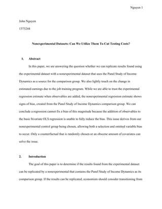
To reinforce how substantial this change is to the treatment, we look at the mean value of
each observable in the nonexperimental dataset we find in Table 2 columns 1 and 2. The
differences, found in column 3, between the treatment group and the comparison is clear. Every
observable has a p-value that is infinitesimally close to zero. It is clear that this comparison
group can not be used as a valid counterfactual.
4. Methods
We perform a regression analysis and give the workers an estimate of the treatment
effect. Our first important regression is on the equation:
TreatEarnings78i = β0 + β1 i + ui
By regressing this equation with only the treatment observable present, we can
understand the effect the training has solely on a participant’s estimated earnings. We then add a
covariate, education. Then we add another, and another. We keep adding covariates until we
reach our final equation:
Treat Educ β Black HispanicEarnings78i = β0 + β1 i + β2 i + 3 i + β4 i
β Married Nodegree Age Earnings75+ 5 i + β6 i + β7 i + β8 i + ui
Our reasoning for adding covariates one at a time is simple: we need to fully measure the
effect each covariate has on the treatment effect. While we have a strong inkling that the estimate
we find from our regression of the experimental dataset gives us what is considered the “true”
5. Nguyen 5
treatment effect, we still systematically add in covariates to see if it greatly changes the treatment
effect.
The results we are expecting from the experimental dataset are the treatment effect is
positive and remains relatively the same as every observable is added to the basic bivariate OLS
regression. This pattern would imply the RCT is successful in finding the true treatment effect.
The results we are expecting from the nonexperimental dataset is the treatment effect will be
negative because the comparison group is not identical to the treatment group and make, on
average, significantly more. We also expect the effect will come closer and closer to the
treatment effect in the experimental dataset with each additional covariate. This pattern would
imply that you cannot use a nonexperimental dataset to replicate results we find from the
experimental.
5. Results
The results we find from regressing the treatment effect on our estimated earnings in
1978 are what we would expect from the experimental dataset. Looking at Table 3 column 1, the
change in estimated earnings for 1978 from receiving the job training, is $886.30.
We believe the treatment coefficient is significant at the 10% level, given the p-value is
less than 0.10. With each covariate added to the regression, the effect the treatment has on
earnings in 1978 remain relatively firm with the exception when Table 3 column 6, the
coefficient related to the no degree observable, is added. However, since the no degree
observable is the only observable to have an implausible p-value, we can look past this minor
inconsistency as long as we account for it in further studies.
6. Nguyen 6
If adding covariates does not change the treatment effect significantly, that means we
found the true treatment effect and we have no omitted variable bias. With all the covariates
added, the treatment effect comes to $806.51, found in Table 3 column 1. We have little reason
to believe our estimated treatment effect of $806.51 is biased because we properly designed our
participants to be randomly assigned treatment and control group eliminating any chance of
omitted variable bias being correlated to our treatment. Seeing as our average earnings for the
treatment group is $5090.05 in Table 3 column 9, around a 16% increase in income is
statistically significant.
The same cannot be said for the regression on the nonexperimental dataset. Looking at
Table 4 column 1, the change in estimated earnings for 1978 from receiving the job training, is
$-16375.02. We believe the treatment coefficient is significant at the 1% level, given the p-value
is less than 0.01. The first issue to address is how can a participant owe money solely from a
working aspect. That, in itself, is enough reason to throw out the results found from this
nonexperimental dataset. The estimate seems to suffer from the selection bias and omitted
variable bias, relegating this estimated treatment effect to be both statistically insignificant and
biased.
With each additional covariate, the $-16375.02 estimate comes closer and closer to the
true estimate of the treatment, $806.51. It does so because our regression is trying to find the
“true” treatment effect of ~$800 found in Table 1. By the end, the treatment effect on estimated
earnings in 1978 is $-2188.05, found in Table 4 column 1, and is significant at the 5% level,
given the p-value is less than 0.05. This estimate is a far cry from the $-16375.02, but still
unacceptable as a successful replication of the experimental dataset results. We have concrete
7. Nguyen 7
evidence that our treatment effect is biased because of the selection bias and omitted variable
bias from using the Panel Study of Income Dynamics as our control group instead of randomly
providing job training.
We could, theoretically, get the experimental estimate by adding more covariates to the
nonexperimental regression. However, issues with this decision is we limit our degrees of
freedom. The larger our degrees of freedom is, the larger our standard error becomes. This will
allows a larger amount of numbers to be answers, weakening the validity of our results and
causing this experiment to be a waste of resources. There is also the practical issue of adding
more covariates increases the cost of our experiment.
6. Conclusion
In this paper, we answered that it is not possible to replicate results found from an
experimental dataset with a nonexperimental dataset. We provide evidence on this belief from
regressing the experimental and nonexperimental dataset. While the experimental regression
estimate with observables shows no obvious biases, the nonexperimental regression estimate
shows signs of selection bias and omitted variable bias. The culprit for this bias seems to
originate from the inclusion of the Panel Study of Income Dynamics as our control group. We
demonstrated that turning a basic bivariate OLS regression into a full multivariate OLS
regression cannot hope to fix this bias because it does not address the faulty control group. With
this control group allowing both the selection and omitted variable bias occur, only a
counterfactual that has randomly assigned participants can negate the bias.
8. Nguyen 8
While it is easier to dissect how the selection bias occurs and how to prevent it from
ruining our estimate of the treatment effect, the omitted variable bias is a different case. While
we can avoid the omitted variable bias in experimental datasets because of randomly assigned
control groups, nonexperimental cannot. They’ll have their error term correlated with the
regression.
Omitted variable bias is also hard to discern from the regression. This stems from the fact
that there can be tens, even hundreds of observables we unconsciously omit from the regression.
Omitting whether a participant has a reliable mode of transportation can negatively affect his
estimated earnings for 1978. Without good transportation, job opportunities with good pay for
the participant are hard to find. Omitting a participant’s transportation or lack of transportation
can be irrelevant in his earnings. This covariate can be intentionally omitted as well. We can add
an endless amount of covariates to eliminate the omitted variable bias. However, applying more
observables adds to the cost of a study. As long as we have the major observables, the study
should be relatively precise many would argue. All in all, as economists, we have to balance the
amount of OVB in a study with how much funding is given for the study and hopefully put that
money to better use in others.
9. Nguyen 9
7. Tables
Table 1: Means of the sample characteristics in the treatment and control groups
from the experimental dataset
Column 1 Column 2 Column 3 Column 4
Variable Control Mean
( )μC
Treatment Mean
( )μT
Difference P-Value
Age 24.45 24.63 -0.18 0.72
Education 10.19 10.38 -0.19 0.14
Black 0.80 0.80 -0.0013 0.96
Hispanic 0.11 0.094 0.019 0.42
Married 0.16 0.17 -0.011 0.70
No Degree 0.81 0.73 0.083 0.0077
Earnings
in 1975
3026.68 3066.10 -39.42 0.92
10. Nguyen 10
Table 2: Means of the sample characteristics in the treatment and control groups
from the nonexperimental dataset
Column 1 Column 2 Column 3 Column 4
Variable Control Mean
( )μC
Treatment Mean
( )μT
Difference P-Value
Age 35.13 24.63 -10.51 < 0.01
Education 12.29 10.38 -1.91 < 0.01
Black .23 .80 0.57 < 0.01
Hispanic .03 .09 0.064 < 0.01
Married .87 .17 0.70 < 0.01
No Degree .28 .73 0.45 < 0.01
Earnings
in 1975
19103.34 3066.10 16037.21 < 0.01