Kostadinov.T._6346839._MSc.BS

0 | P a g e
UNIVERSITY OF AMSTERDAM - FACULTY OF ECONOMICS AND BUSINESS
Mean variance
convergence in the EU
Master Thesis
Msc. Business studies
Author: Todor Kostadinov Kostadinov
6346839/10085726
Supervisor: Dr. Jeroen Ligterink
Second reader:
August 30-th, 2012

1 | P a g e
Abstract
In this Master thesis I research the mean variance characteristics of national stock markets
of the EU. I take a sample of 16 old EU member states and 5 new member states, which I
examine over the period 1993 – 2010. I use the Euclidean distance as a two-fold measure of
dissimilarity and study its time trend. I report that historical real term mean variance
characteristics of the old EU member states have not converged whereas convergence occurred
among the new member states. I attribute these results largely to the impact of volatility. Further I
introduce the unlevered for volatility mean variance distance – a novelty to the seminal approach
of Eun and Lee (2010) on this topic. I study a few possible information channels for the speed of
convergence and report that it is largely predicted by the initial dissimilarity – a finding for which
I find no theoretical reasoning. In 17 years the mean variance characteristics of the old member
states have become more similar by nearly a third and the same is valid for the new member
states but achieved in twice shorter time. Next I apply the Heston and Rouwenhorst (1994)
approach and report a significant decrease in country effects in the documented mean variance
convergence after control for volatility, which I associate with stock market integration. Finally I
examine the impact of the increasing mean variance similarity on the investment opportunity set
and report that it exerted negative impact much in the same way as the increasing international
correlations of returns.

2 | P a g e
TABLE OF CONTENTS
1. Introduction .................................................................................................................................................4
1.1 Background of this research ..................................................................................................................6
1.2 Literature review ...................................................................................................................................6
1.2.1 On the international correlation structure of equity returns............................................................6
1.2.1.1 Why diversify internationally? ....................................................................................................6
1.2.1.2 Is the international correlation structure constant over time? ......................................................7
1.2.1.3 Why this research? ......................................................................................................................8
1.2.2 On the EU financial market integration..................................................................................................9
1.2.2.1 Model and common return factor – based approaches to integration ..........................................9
1.2.2.2 News – based approaches to integration....................................................................................10
1.2.2.3 Quantity – based approaches to integration...............................................................................11
1.2.2.4 Price – based approaches to integration.....................................................................................11
2. Theory and evidence behind hypotheses ...................................................................................................12
2.1 Financial market integration and equity return fundamentals. ............................................................13
2.2 Volatility and its impact on returns .....................................................................................................14
2.3 Information channels for the speed of convergence ............................................................................14
2.3.1 Initial dissimilarity........................................................................................................................14
2.3.2 Market size ...................................................................................................................................15
2.3.3 Dividend yields.............................................................................................................................16
2.3.4 Negative volatility ........................................................................................................................16
2.4 Country versus industry effect in equity returns..................................................................................17
2.5 The impact of the mean variance convergence on the investment opportunity set..............................17
3. Methodology and dataset...........................................................................................................................18
3.1 Methodology .......................................................................................................................................18
3.1.1 (Similar) Previous measures of stock market convergence ..........................................................18
3.1.2 The Euclidean distance as a two dimensional measure of dissimilarity .......................................18
3.1.3 Estimation procedures for the Euclidean mean variance distance ................................................19
3.1.4 The volatility correction ...............................................................................................................22
3.1.5 Time trend investigation procedures ............................................................................................23
3.1.6 Procedures taken on hypotheses H4.1-4.......................................................................................24
3.1.7 Procedures on country versus industry effect research.................................................................27
3.1.8 Procedures on examining the investment opportunity set ............................................................29
3.2 Dataset.................................................................................................................................................30
4. Results .......................................................................................................................................................31
4.1 H1: The historical mean variance characteristics ................................................................................31
4.1.1 H1.1: The historical mean variance characteristics in the old member states...............................31
4.1.2 H1.2: The historical mean variance characteristics in the new member states ............................33
4.2 H2: The mean variance characteristics unlevered for volatility ..........................................................34
4.2.1 H2.1: The mean variance characteristics unlevered for volatility in the old member states.........34
4.2.2 H2.2: The mean variance characteristics unlevered for volatility in the new member states .......37
4.3 H.3: The effect of volatility on the historical mean variance characteristics.......................................40
4.3.1 H3.1: The effect of volatility on the historical mean variance characteristics in the old
member states........................................................................................................................................40
4.3.2 H3.2: The effect of volatility on the historical mean variance characteristics in the new
member states........................................................................................................................................41
4.4 Channels of information for the mean variance convergence..............................................................42
4.4.1 H4.1: The initial distance and its effect on the speed of convergence..........................................42
4.4.2 H4.2: The stock market size and its effect on the speed of convergence......................................43
4.4.3 H4.3: The long term trend in dividend yield dissimilarity on the speed of convergence .............43
4.4.4 H4.4: Negative volatility and its effect on the mean variance convergence .................................44

3 | P a g e
4.5 H5: Country versus industry effect on the mean variance characteristics after control for volatility..45
4.6 H6: The effect of the mean variance convergence on the investment opportunity set. .......................47
5. Conclusion.................................................................................................................................................49
6. References .................................................................................................................................................53
7. Appendix ...................................................................................................................................................58

4 | P a g e
1. Introduction
1.1 Background of this research
In this paper I evidence for diminishing differences in the mean variance characteristics of
national European stock markets and attribute them to be another manifestation of the financial
market integration in the European Union. The last 20 years are marked by two phenomena in the
European investor’s practice – a continuing rule of the mean variance optimization model and an
unprecedented integration of European national financial markets. My research finds ground in
these two widely accepted paradigms of the present day.
In his 1952 and 1959 works Markowitz mathematically proves his theory that a risk-
averse investor would optimize his selection by choosing from an efficient frontier in order to
maximize return given certain level of risk and minimize risk under a certain level of return. The
essence of his theory is that the portfolio variance is a function of the co-movements of its
constituent stocks and can go below the individual variance of any of the latter. This is where he
seeks explanation for the common investment practice for diversification instead of investing in
the single stock with the highest expected return and minimum risk. Thus mean, variance and
equity correlations and co-movements became the three building blocks of Modern Portfolio
Theory.
While Markowitz suggested an explanation for the behavior of the individual risk averse
rational investor, the works of Sharpe (1964), Lintner (1965) and Black (1972) developed it into a
model for economic equilibrium where all investors behave as the Markowitz rational risk averse
investor. This is what today is referred to as the Capital Asset Pricing Model (CAPM).
Despite the widespread criticism for its poor empirical support, even its loudest opponents
Fama and French admit that the “CAPM is still widely used in applications, such as estimating
the cost of capital for ﬁrms and evaluating the performance of managed portfolios. It is the
centerpiece of MBA investment courses. Indeed, it is often the only asset pricing model taught in
these courses.”
Hence I believe that my Master’s thesis will have scientific value as it researches the very
foundations of this widespread model. In the literature review that follows below I show that

5 | P a g e
much attention has been paid to the changing correlation structure of national stock markets over
time, but not to their mean variance attributes. Therefore a scientific gap in literature exists on the
mean variance pattern of behavior of national European stock markets, its origin and
consequences. My work attempts to fill this gap.
The other side of this literature gap lies within the context of the European financial
market integration. Since the end of World War II the countries of west Europe have gradually
worked towards the establishment of the common European market where people, commodities
and capitals move freely and the rule of one price applies. Much has been done to facilitate this
process in the financial sector namely: the introduction of the European Monetary System (EMS)
that coordinates monetary policy through its Exchange Rate Mechanism (ERM); the introduction
of the Second Banking Directive (1989), the Capital Adequacy Directive (1993) and the
Investment Services Directive (1993) which sought co-integration of national financial sectors;
the introduction of the Stability and Growth Pact (1997) that aims to maintain fiscal discipline
and finally the adoption of the Economic and Monetary Union (EMU) under the regulation of the
common supranational institution of the European Central Bank (ECB). These are all widely
cited pillars of the financial sector integration within the EU. The literature review that follows
below evidences equity market integration in addition to integration in the other financial sectors
such as money markets, government and corporate bond markets and bank credit markets.
Following the basic intuition of the “rule of one price” the cost of equity should converge to a
common EU wide level. If assets are priced equally throughout the EU, then a convergence in
equity valuations can be expected as they directly reflect the cost of equity convergence.
Therefore a similar convergence in the core characteristics of asset returns such as mean value
and standard deviation is also expected. In my research I look at the mean variance distance of
EU national stock returns and try to find the effect of EU stock market integration reflected in its
behavior. Furthermore a process of integration would imply a decrease in national idiosyncratic
effects. In part 4.5 I try to prove this is valid for the mean variance characteristics of national
stock markets and that it is in fact the driving force behind their documented pattern of behavior.
Essentially I study how stock market integration of the EU also translates into more similar mean
variance characteristics and what that implies for the EU stock market investor.

6 | P a g e
I do so by applying a simple price based and model free approach that builds straight on
data from stock markets. Firstly I collect return series from Level one national stock returns from
DATASTREAM. Then I estimate the Euclidean mean variance distance as a two-fold measure of
cost of equity dissimilarity across national indices and study its behavior over time applying
regression analysis on the time variable. Further I document the effect of volatility and report that
its increased levels accompanying the world financial crises after 2008 were and obstacle to a real
term convergence in the mean variance distance of EU national stock markets. I therefore
eliminate the effect of volatility and report convergence in the unlevered for volatility mean
variance distance. Next I investigate a few possible information channels for the reported speed
of convergence namely stock market size, dividend yield dissimilarities and bear market state. I
also report that the “champions” in convergence where the most dissimilar countries in the
beginning of the sample. Further I try to prove that the convergence in the mean variance space
can really be attributed to stock market integration. I do so following the methodology of Heston
and Rouwenhorst (1994) by which I split out country and industry effects. I report a significant
decrease in national idiosyncratic effect which is suggested by integration theory and therefore
claim that the pattern of behavior of the unlevered for volatility mean variance distance can be
attributed to the equity market integration throughout the EU. Finally I study the effect of the
reported phenomenon on the investment opportunity set and compare it to the increasing return
correlations effect. I find that both effects exert negative impact.
The remainder of this paper I organize as follows. In Chapter 1.2 I summarize relevant
literature. In Chapter 2 I provide relevant theory and motivate my hypotheses. In Chapter 3 I
define my dataset and methodology. In Chapter 4 I report and discuss my results. In Chapter 5 I
conclude.
1.2 Literature review
1.2.1 On the international correlation structure of equity returns
1.2.1.1 Why diversify internationally?
Levy and Sarnat (1970) claim “that if equities are perfectly correlated, no amount of risk
can be diversified”. Naturally any group of stocks from one country would be much more
correlated than the stocks from different countries in a segmented financial world where domestic

7 | P a g e
factors dominate global factors. A whole new flow of research stems from here. Grubel (1968)
studies the returns, variances and correlations of eleven stock markets. Then he compiles two
potential portfolios – one including only the countries of the Atlantic basin and one adding Japan,
Australia and South Africa to the former. Both portfolios offer greater return at the same amount
of risk faced by an American investor, but the first portfolio does so with an 18.7% increase
whereas the second with a 68% increase. Explanation for these results he seeks in the higher level
of correlation of returns in the former and the lower in the latter. Similar are the results for the
reduction of risk. His conclusion is obvious - future international diversification of portfolios is
profitable and more of it will take place. Levy and Sarnat (1970) increase their sample to 28
countries and conclude that the majority of optimal portfolios include developing markets, which
again is explained by the relatively low correlations of their returns. Solnik (1974) estimates that
the well diversified American investor can reduce his risk exposure up to 50% and the typical
American investor can save a whole 90% by sole international diversification. Grauer and
Hakasson (1987) apply a multi-period portfolio model different from the mean variance model
for portfolio selection used by the previous authors, and again come up with similar results –
there are substantial gains from adding non-US stocks to the portfolio of an American investor
and there is serious evidence for market segmentation. There are of course those who question
international diversification. Sinquefield (1996) builds on Fama and French (1993) 3-factor
model and argues that an investor is driven by the factors size and value – when they diversify
internationally, investors are doing nothing else but picking size and value stocks from different
geographical regions.
1.2.1.2 Is the international correlation structure constant over time?
In a world where correlations between national stock markets are the source of
diversification gains a variety of researchers try to quantify them and understand their nature.
Early researchers such as Panton et al (1976), Watson (1980), Philippatos (1983), Ratner (1992)
and others maintain that correlations between country equity indices are stable over time. On the
other side researchers like Kaplanis (1988) start questioning this. Kaplanis (1988) studies 10
national markets over 1967-82 and concludes that their correlation matrices are stable over time
but the covariance matrices are not. Further research evidences that with the advance of
globalization country specific factors become dominated by global factors especially in times of

8 | P a g e
increased volatility. Thus international correlation is viewed by many as time and volatility
variant – Koch and Koch (1991), King, Sentana and Wadhwani (1994), Bertero and Mayer
(1990), Longin and Solnik (1995) – all of these papers investigate the effect of 1987 crash on
correlation nature of markets. Such conclusions are supported also from alternative approach of
Solnik and Roulet (2000) who use the cross-sectional dispersion as a measure of correlation level
versus the standard use of time series. As the majority of researchers claim increasing country
correlations, diversification over countries becomes less attractive compared to diversification
over industries. Cavaglia et al.(2002) report that for the period between 1995 and 1999
diversification on industry was a better option for reducing variance. Similar are the findings of
Brooks and Catao (2000) and L’Her et al. (2002).
1.2.1.3 Why this research?
The literature review provided so far shows how much attention has been paid to the
correlation structure of international markets. Little investigation has been done on the mean
variance characteristics of the same markets. Although it sounds appealing that markets with
increasing correlation of returns should also exhibit increasingly similar mean variance
characteristics, this is not necessarily so. In their research on the mean variance characteristics of
17 developed stock markets Eun and Lee (2010) define mean dissimilarity, variance dissimilarity
and correlation of returns between a market and the world market as:
| ( ) ( )| | ( ) ( )| ( )
| ( ) ( )| |( ) ( ) ( )| ( )
( )
√
( )
( )
( )
From (1) (2) and (3) they argue that higher beta always increases correlations while the
mean and variance differences decrease only when the beta is less than unity. In fact they report
that while the average cross market level of correlation increased during the investigated period,
most of their sample countries exhibited mean variance convergence while others exhibited no

9 | P a g e
time trend and Japan essentially diverged in terms of mean and variance from the rest of the
sample. Hence they argued that increasing correlations and the growing similarities in the mean
variance characteristics they report are two distinct phenomena – correlations do not necessarily
imply similarity. If national stock markets of the EU are co-moving together increasingly
similarly, then are their mean variance characteristics also converging? This paper tries to answer
this question, to explain the documented pattern and seek its consequences.
1.2.2 On the EU financial market integration
There is a wide academic agreement on three general gains from financial integration – an
increase in risk sharing and diversification opportunities, an enhanced capital allocation
environment and higher growth opportunities. These and the above described cornerstones of
European economic integration are among the prime reasons for the extensive academic research
in European financial integration (Baele et al. (2004).
Researchers address the matter of equity market integration in Europe using four broadly
defined methodological approaches namely model and common return factor – based, news –
based, quantity – based and price – based approaches.
1.2.2.1 Model and common return factor – based approaches to integration
Among these fall the studies which try to determine to what extent the variation of local
returns is explained by a common global factor. Researchers like Bekaert and Harvey (1995),
Dumas and Solnik (1995), Ferson and Harvey (1991), Hardouvelis, Malliaropoulos and Priestley
(2000b) (2006), Stulz and Karolyi (2001) define integrated markets through capital asset pricing
models with the following general formula:
( ) ( )

10 | P a g e
In these models markets achieve integration once λd reaches zero. In this case the price of
local portfolios depends entirely on the non-diversifiable global risk and local idiosyncratic
factors exert zero influence.
In their study on European equity market integration Hardouvelis, Malliaropoulos and
Priestley (2006) report that the relative importance of European wide factors increases with the
probability of joining the Euro zone. Their findings suggest that the degree of stock market
integration changes over time and is largely predicted by the interest rate differentials of a
country with Germany. In their model the national stock markets of Europe practically fully
converged immediately before the introduction of the Euro. They also claim that the cost of
equity decrease from 0.5 to 3.0 % in different industries as a consequence of equity market
integration in the old continent. The major drawback of these methodologies is that they
explicitly assume an asset pricing model. Thus these studies face the double challenge of the joint
hypothesis test – they have to prove both the validity of their models, on which there is normally
a wide disagreement, and prove their integration hypothesis.
Another similar strand of studies tries to distinguish between the country and industry
factors on local equity returns. Where a decrease in country effect is presented, this is considered
a sign of market integration. In their seminal work Heston and Rouwenhorst (1994) claim that
global industry factors explain only 4 % of national stock return variation. Nevertheless
following their ideological framework more recent studies such as Baca et al. (2000), Cavaglia et
al. (2002) and Brooks and Del Negro (2002) evidence for a relative rise of industry effect versus
a decrease in national idiosyncratic effects.
1.2.2.2 News – based approaches to integration
Through their news – based approaches authors try to be more informative about the
dynamics of the integration process and its specific drivers – a major methodological drawback
of the previous approach. This approach is pioneered by Bekaert and Harvey (1997). In their
paper the authors report that the percentage of local equity variance explained by common news
increases with their measure of financial integration. Further researchers such as Baele (2005)
report that at the end of the 1980-ies the sensitivity of 13 European equity markets towards
aggregate US and European returns increased. In a similar manner Fratzscher (2002) studies

11 | P a g e
volatility spillovers and claims that the elimination of exchange rate volatility and monetary
policy convergence lead to an increased level of correlations on Euro area stock markets.
1.2.2.3 Quantity – based approaches to integration
The third strand of studies looks at the reduction of the so called “home equity bias” as a
sign of stock market integration. The technological progress in telecommunication; the
consolidation of Dutch, Belgian and French exchanges into Euronext in 2000 are strongly
facilitating cross border trading in Europe. The introduction of the single European currency
eliminated exchange risk as well as the limitations on insurance companies and pension funds to
hold assets denominated in local currency. This triggered a spur of cross border equity investment
which is also academically reported. For example Adam et al. (2002) reports that for the period
1997 – 2001 investment funds in the Euro zone increased the part of their assets allocated on a
Europe-wide strategy substantially surpassing 50% at the end of the studies period. The same
study also documents similar evidence in pension funds policy where a constant percentage of
foreign equity is held for the period 1992 – 1998, but it rose significantly after 1999.
1.2.2.4 Price – based approaches to integration
Finally the price – based models derive their methodological mainframe in the “law of
one price”. If equity market integration is going on, then equity returns should become more and
more similar and converge to a common European wide discount rate. Therefore signs of equity
market integration should be apparent directly on the equity markets themselves. Some studies
see stock market integration through increasing international return correlations. Such are the
works of King and Wadhwani (1990), Koch and Koch (1991) and many others. Authors such as
Adjaoute and Danthine (2003) study country versus industry return correlations and return
dispersions over time and consider the rising trend of the former as a sign of stock market
integration. Inversely Roulet and Solnik (2000) study cross-sectional dispersion and regard its
diminishing trend in country returns as a sign of equity market integration. Among the merits of
such approaches is the fact that they are model free and based on data observed on the actual
stock markets.
In their research on equity market integration in the EU, Bekaert et al. (2012) employ an
approach which is similar to the price – based methods. They build on the idea that financial and

12 | P a g e
economic integration is reflected in the earning yield valuation ratio through the influence of
discount rates and growth rates. Then they build a segmentation measure as the absolute
difference in earning yields of similar industries located in different countries in Europe. Their
findings are that EU membership leads to significant reduction of the valuation differentials,
while Euro zone membership played a much less significant role.
My work follows the concept of the last group of methodologies as mean value and
variance of returns are sources of information taken directly from stock markets which brings my
work closer to the price – based methodologies. My measure of dissimilarity resembles the one
used by Bekaert et al. (2012) namely the absolute distance in the earning yield valuation ratios.
My work is also similar in concept to Roulet and Solnik (2000), whose measure of dissimilarity is
the dispersion of returns. Particularly I follow Eun and Lee (2010) and use their suggestion for
dissimilarity measure namely the Euclidean distance between mean and variance. My work also
resembles the works of as Baca et al. (2000), Cavaglia et al. (2002) and Brooks and Del Negro
(2002) all of whom refer to Heston and Rouwenhorst (1994) methodology to separate country
and industry effect. In my case I do so in order to attribute the reported convergence in mean and
variance to the widely reported stock market integration within the EU.
As stated above I follow the methodology of Eun and Lee (2010) who carried a similar
research on the mean variance attributes of developed versus emerging markets. Unlike them I
change my sample countries to the EU member states and differentiate between old member
states and new member states. I apply higher frequency of observations and limit my time scope
to 1993 – 2010 thus concentrating on the period immediately following the creation of the EU
and capturing post 2008 period. In addition my study essentially reports the behavior of the mean
variance Euclidean distance unlevered for volatility which is a novel variable qualitatively
different from the historical mean variance distance on which they report.
2. Theory and evidence behind hypotheses
In this research I distinguish between two groups of EU member states as theory suggests
they share different stock market characteristics. These are namely the group of the old EU
member states and the group of the new member states. The first three hypotheses that follow I
shall investigate in both samples putting the same theoretical reasoning and employing the same

13 | P a g e
methodology. Therefore for H1, H2 and H3 explained in Chapter 2 I shall report two hypotheses
subsets in Chapter 3 Results: 1 and 2 for the group of the old member states and the group of the
new member states accordingly. Further I shall try to draw comparison between the behaviors of
both country samples as it may contain valuable information.
In this Master’s thesis hypotheses H2 and H5 are the centerpieces of the research – from
their results I conclude on the mean variance convergence in the EU (H2), the integration of stock
markets as its driving source (H5) and in H6 I seek for possible practical implications.
2.1 Financial market integration and equity return fundamentals.
The famous CAPM states that the cost of equity is a function of the risk free rate
(commonly accepted as government bond rate) and the covariance of the risky asset (the stock’s
beta) with the rate of return on the market portfolio (the equity market premium). Assuming
there are no structural breaks in the risk aversion of investors, the behavior of the cost of equity is
only dependent on the trend in government bond rates and equity risk premiums. Focusing on the
government bond rates which reflect sovereign risk, one can expect that the introduction of the
single European currency as well as the voluminous legislative convergence throughout the EU
preceding 1999, lead to a convergence in government fiscal policies, national banks monetary
policies and elimination of currency risks. These are all important requisites for convergence in
government bond rates (the risk free asset), which is indeed a well academically evidenced
phenomenon (Adam et al.(2002), Baele et al.(2004)).
Looking at the market premium part of equity returns one can expect that in a perfectly
segmented market the marginal investor will require compensation for his undiversified portfolio.
In a perfectly integrated market the marginal investor will hold a diversified portfolio with much
less undiversified risk left to require compensation for. Adjaoute and Danthine (2003) report that
the systematic risk as measured by the standard deviation of returns is smaller in MSCI EMU
index versus all else MSCI Euro-zone member indices. Further if the law of one price holds,
assets that produce the same cash flows and are exposed to same amount of risk, should be priced
equally on an integrated efficient market that provides equal access to all investors. Hence equity
market returns are expected to become more and more similar which is also the claim of many
price – based studies such as Roulet and Solnik (2000), Adjaoute and Danthine (2003), Bekaert et

14 | P a g e
al. (2012). In light of this theoretical evidence a convergence in the mean variance space is
expected as they are key characteristics of equity returns on stock markets for whose financial
integration there is a vast amount of evidence. I therefore state the following two hypotheses:
H1: The historical mean variance characteristics of national stock markets within the EU
are converging.
H2: The mean variance characteristics of national stock markets within the EU are
converging when volatility is accounted for.
2.2 Volatility and its impact on returns
As mentioned above theory suggests positive connection between volatility and stock
return correlations. Such are the claims of King and Wadhwani (1990), Bertero and Mayer
(1990), Longin and Solnik (1995), Karolyi and Stulz (1996) all of who study changing
correlation structures by comparing unconditional correlations across various sub periods or by
examining conditional time varying correlations. Ramchand and Susmel (1998) apply a
switching autoregressive conditional heteroskedasticity (SWARCH) model and conclude
qualitatively similarly – the correlations of the US stock market with other stock markets are
significantly higher during times of increased variance. In line with this theoretical evidence I
hypothesize that:
H3: Volatility exerts influence on the historical mean variance characteristics in the EU.
2.3 Information channels for the speed of convergence
Following the acceptance of H2 on cross market level I try to find explanation for the
different speeds of convergence on national level. I consider the following few information
channels.
2.3.1 Initial dissimilarity
For this information channel I fail to find any theoretical explanation, which is why it is
arguable to what extent the reported statistical association is a sign of true economic causality.
Nevertheless the statically significant results open the doors for future research in this field.

15 | P a g e
Furthermore the results that follow are in line with previous reported findings of Eun and Lee
(2010).
H4.1: The initial mean variance difference between a national stock market and the cross
market mean variance characteristics explains the reported speed of convergence of mean
variance characteristics.
2.3.2 Market size
Size effect is a well-known topic in stock market literature. On firm level Banz (1981)
first reported that small companies have bigger risk-adjusted returns compared to the big
companies. This was later confirmed also by Fama and French (1992). According to Heston,
Rouwenhorst, and Wessels (1995) big size also brings lower cost of capital regardless of the
company beta. On market level size effects are recognized by Asness, Liew and Stevens (1997)
who construct country portfolios based on market size and report that small market size portfolios
outperform big market size portfolios. Another widely covered topic related to market size is
cross listing of companies from smaller markets on the exchange floors of countries with bigger
markets. Foerster and Karolyi (1999) state that trading on bigger and more developed markets
increases the shareholders base of a company which results in lower cost of equity. Lins,
Strickland, and Zenner (2000) argue that bigger stock markets provide greater liquidity and
foreign companies migrate there gaining access to more capital and cash flow independence.
Another acknowledged advantage of big markets is higher investor protection which reduces
agency costs (La Porta, Lopezde-Silanes, Shleifer and Vishny (2000). If financial deregulation
dictates a migration from smaller to bigger more efficient markets, this could have a profound
impact on stock market returns through the betas of local markets to common integrated market
portfolio. This will be the result of the relatively lower liquidity and diversification options left
on small local markets versus the increased potential on big markets. In light of this previous
research I investigate whether markets with different size behave differently including in terms of
integration with other markets. I hereby hypothesize that:
H4.2: Stock market size explains the reported speed of convergence of mean variance
characteristics.

16 | P a g e
2.3.3 Dividend yields
In line with theory in 2.1 suggesting both risk free rate and equity risk premium
convergence in the context of financial market integration, one can look for possible channels of
information in the dividend yield trends. Rozeff (1984) first stepped on the famous Gordon –
Shapiro (1956) model and a made a claim that:
( )
where:
–
–
His findings where later confirmed by Fama and French (1988). Damodaran (2012) also points
this method as a statistically significant predictor of the equity risk premium. In addition Bekaert
and Harvey (1995) introduce an asset pricing model where the advance of market integration
changes over time. In their model they claim that more integrated markets share lower dividend
yields. In my research I address the question whether markets exhibiting more similar dividend
yields are also converging faster towards mean variance similarity. Hence I hypothesize that:
H4.3: The time trend in dividend yield differences explains the reported speed of mean
variance convergence.
2.3.4 Negative volatility
Longin and Solnik (2001) document significantly higher correlation of returns in the
times of negative stock market trends. Similar are the findings of Koch and Koch (1991), King,
Sentana and Wadhwani (1994), Bertero and Mayer (1990), Longin and Solnik (1995). During the
investigated period there where two periods of extreme downside volatility – the late 1990-ies
and the 2008 crash, hence I investigate whether and to what extent the current state of market
trend influences the similarities between stock markets in terms of mean and variance.
H4.4: The reported speed of mean variance convergence state variant, state distinguished
between bullish or bearish market.

17 | P a g e
2.4 Country versus industry effect in equity returns
In his seminal research Solnik (1974) lays the foundation of international diversification
which he claims reduces more risk than diversification over industries. Despite the numerous
studies reported in the literature review which document a growing international correlation of
returns, authors such as Heston and Rouwenhorst (1994) and Griffin and Karolyi (1998) maintain
that country factors still dominate industry factors. On the other hand Cavaglia et al. (2002) and
others claim an increasing role of industry factors. Furthermore authors such as Baca et al. (2000)
and Brooks and Del Negro (2002) claim that country effects are already playing a diminishing
role stock market returns, which is in line with international financial market integration.
Following the acceptance of H2 I research whether the mean variance convergence can be
attributed to two potential reasons suggested by theory – a declining country effect and a rising
industry effect. If the stock markets of the old EU member states have become more similar in
mean and variance and empirical evidence is for a declining country effect, then mean variance
convergence could be explained by stock market integration within the EU. In this section I
investigate this matter. Hence my hypothesis:
H5: The mean variance convergence reported after controlling for volatility is evidence
for stock market integration within the EU.
2.5 The impact of the mean variance convergence on the investment opportunity set
As outlined in the theory above increasing correlations of returns exhibit negative effects
on the diversification gains and from here on the overall portfolio performance. More similar
mean and variance could also exert a negative impact on the investment opportunity set much in
the same way as the increasing correlations do. Yet do they really, to what extent and in which
direction? In this section I hypothesize that:
H6: The mean variance convergence exerts influence on the investment opportunity set.

18 | P a g e
3. Methodology and dataset
3.1 Methodology
3.1.1 (Similar) Previous measures of stock market convergence
In their study on growth and income Barro and Sala-i-Martin (1991) introduce the falling
over time cross-sectional variance of a variable as σ-convergence. Many economic researchers
follow their example in a vast variety of research fields all termed as “Barro” regressions. In their
studies commissioned by the ECB Adam et al. (2002) and Baele et al. (2004) classify this
approach as price indicators and recommend them as benchmark for credit and bond market
integration. A number of researchers apply this methodology in their study on stock market
integration. Erdogan (2009) finds evidence of σ-convergence both on country and industry levels
between five of the old EU-member states. Babetskii et al. (2007) extend their study on five of
the new member states and also find evidence for of σ-convergence in their stock markets
although in the least degree as compared to the convergence in bond market, foreign exchange
and money markets.
3.1.2 The Euclidean distance as a two dimensional measure of dissimilarity
In my research I try to prove that the mean variance characteristics of national European
stock markets are gradually becoming more similar. I do so by defining a measure of
dissimilarity which I regress on the time variable expecting to see a negative trend, which implies
a declining (increasing) dissimilarity (similarity).
Particularly I follow Eun and Lee (2010) and use their measure of dissimilarity namely
the Euclidean distance, which is a common tool of cluster analysis. This approach is similar in
concept to the σ-convergence and dispersion methodologies discussed above, but also
accommodates the following advantages. Firstly it is suitable as short term measure and does not
require long years of observations. In this study I examine the behavior of monthly averaged
weekly returns to calculate the Euclidean distance, but the latter can be estimated over any
frequency, this allowing it to be used successfully as a short term predictor and serve as a
practical information tool for investors. Second it can accommodate the two-dimensional nature
of the investigated subject – mean and variance of stock returns. Third the distances (similarities)

19 | P a g e
are not so sensitive to the inclusion of outliers. Last but not least, as with most cluster analysis
tools (Tryon (1939)) it can distinguish data structures without providing any specific
interpretation or in other words - no asset pricing models have to be explicitly assumed in order
to draw conclusions. Thus the approach applied in this Master’s thesis tells a story free from any
potential biases which all asset pricing models suffer from.
Once I calculate the Euclidean distance of mean and variance in each period, I build a
time series whose time trend I study applying regression analysis.
3.1.3 Estimation procedures for the Euclidean mean variance distance
As mentioned already the measure of dissimilarity terms of mean and variance I employ
in this study is the Euclidean distance, which is a common tool of cluster analysis. Cluster
analysis was first introduced by Tryon (1939) and since then has developed into a wide variety of
instruments which place objects into groups according to common well defined attributes they all
share. This valuable feature of cluster analysis is often used to provide clues for possible
hypotheses in the exploration periods preceding the research itself. Cluster analysis allows the
“luxury” not to assume any pricing models, which often hides too many caveats in stock market
research.
Clusters are formed by single or multiple dissimilarities (distances) between objects.
Being the geometric distance in a multi dimension space, the Euclidean distance is among the
most widespread distances in cluster analysis. The generic formula of the Euclidean distance is:
√∑( ) ( )
where:

20 | P a g e
I calculate the Euclidean distance each month during the period of the study and observe
its behavior over time. If it significantly decreases over time this means that national stock
market returns are becoming increasingly similar in their mean variance attributes and vice versa.
Particularly in this study I start from returns from Level 1 market indices of
DATASTREAM. First I estimate the weekly returns, their monthly average and their monthly
standard deviations. Then I calculate the Euclidean distance between monthly return mean and
standard deviations for each national market and the average cross market return mean and
standard deviation. Therefore I first introduce the two separate distances that build up to the
Euclidean distance, namely the mean distance and the variance distance.
By mean distance I understand the absolute difference between the monthly averaged
weekly return of one national market and the sample average of national market monthly
averaged weekly returns. For each market m in each month t I apply the following formula:
|̅̅̅̅̅̅ ∑ ̅̅̅̅̅̅| ( )
where:
̅̅̅̅̅̅–
–
I use similar reasoning for the variance distance, which is the absolute difference between
the standard deviation of weekly returns of a national market and the sample average of national
market standard deviations. For each market m in each month t I apply the following formula:
| ∑ | ( )
where:

21 | P a g e
–
–
If the two distances are directly input as calculated above, the Euclidean distance would
suffer from its major methodological drawback. This method does not care about the scales of its
inputs, therefore the ones with greater dispersion can exert bigger influence on similarity
measure. A normalization procedure is applied to overcome this problem where the size of each
variable relative to the sum of both variables is applied as a weight. The weights are calculated as
follows:
( ) √∑ ∑ (∑ ∑ ∑ ∑ )⁄ ( )
( ) √∑ ∑ (∑ ∑ ∑ ∑ )⁄ ( )
where:
( )
( )
Therefore the Euclidean distance is calculated from the weighted mean and variance
distances following the formula:
√( ( )⁄ ) ( ( )⁄ ) ( )
where:

22 | P a g e
As mentioned above I calculate this Euclidean distance for each market m and I average
them to arrive at the cross market mean variance distance. I repeat this procedure during each
month t and build a time series of mean distances, variance distances and Euclidean mean
variance distances both on national and on aggregate cross market level whose behavior I study.
3.1.4 The volatility correction
Once I have the time series of distances as explained above I fail to prove my H1.1 as
evidenced from the time trend graphics and an ordinary least squares regression. As suggested by
the previous literature I look for evidence of volatility influence. To prove my H3 I apply
correlation and ordinary least squares regression analyses:
( )
where:
I report that market volatility and the Euclidean mean variance distance are positively
correlated. Also volatility significantly predicts the Euclidean mean variance distance. This could
potentially explain why there is no observable time trend.
To eliminate the effect of volatility I introduce a novelty modification to the original
methodology of Eun and Lee (2010). I follow the basic intuition of William Sharpe and his
Sharpe ratio, where the excess return is controlled for its risk exposure simply by dividing the
equity risk premium by its standard deviation. I follow this approach and control for volatility
and look at the behavior of the Euclidean mean variance distance unlevered for volatility. In my
case I divide each mean distance and variance distance by the market volatility proxy above. This
way the formula for the newly introduced measure for the unlevered for volatility Euclidean
distance is as follows:
√(
( )⁄
∑ ̅̅̅̅̅̅̅
) (
( )⁄
∑
) ( )

23 | P a g e
where:
3.1.5 Time trend investigation procedures
Since the time trend graphics of the historical Euclidean mean variance distances provides
a self-explanatory evidence for no time trend, I limit my methodology for investigating H1 to a
simple ordinary least squares regression analyses as follows:
( )
My H2 states that convergence occurred in the dissimilarities of mean and variance of
national stock markets within the EU after controlling for volatility. Essentially I regress the time
series of unlevered for volatility mean distances, variance distances and Euclidean mean variance
distances on the time variable and look at the beta coefficient of the following regression
equation applied to each country and on average cross market:
( )
( )
( )
A significantly negative beta of the time variable I interpret as diminishing dissimilarities
and vice versa.
For the regression analysis I use Newey – West regression which overcomes the common
problems of autocorrelation and heteroskedasticity of the error terms in financial time series
analyses.
Before I do so I first apply the Augmented Dickey – Fuller test. The purpose is to cope
with the common time series problem with stationarity. In general non-stationary data lead to
spurious regressions which provide evidence for relationship between variables when one does

24 | P a g e
not exist. If data is found to be non-stationary at 1st
level it needs to be transformed and tested for
stationarity at 2nd
level and so on until stationarity is achieved. The null hypothesis of the
Augmented Dickey-Fuller test is rejected when the t-statistic is smaller than the critical value at
the desired significance level. Before I do the Augmented Dickey-Fuller test I also perform a lag
selection procedure using STATA varsoc command. This syntax reports the Akaike Information
Criterion (AIC) and Schwarz' Bayesian Information Criterion (SBIC) and I take its
recommendation for lag order for each dependent variable accordingly. I use the same lag order
both for the Newey – West heteroskedasticity autocorrelation consistent regression and the
Augmented Dickey-Fuller test.
Thus my time trend investigation procedure for proving H2 (also applied in H4.3 and H5)
assumes a 3-step model – lag selection, stationarity testing and finally a heteroscedasticity and
autocorrelation consistent regression. I apply this methodology to mean distances and variance
distances separately as well as to the Euclidean mean variance distances. I study distances both
on cross market and on national levels. I report convergence hypothesis results both in USD and
in national currencies. The reported intercepts I interpret as initial distances and the slopes I
consider as speed of convergence.
3.1.6 Procedures taken on hypotheses H4.1-4
Once I report the results from the time trend investigation in H2.1, I estimate a pairwise
test for equality of the slope coefficients of the mean variance distance unlevered for volatility. It
essentially reports that countries from the old member states group of the EU converge at
different speeds.
To decide on my H4.1 I apply cross sectional ordinary least squares regression where the
independent variable is the initial distance and the dependent variable is the speed of convergence
of the mean variance distance unlevered for volatility. Both variables are from the Newey – West
heteroskedasticity autocorrelation consistent regressions in the previous section as proxied by the
intercept and slope coefficient accordingly. Specifically follow Eun and Lee (2010) and estimate
the following regression equation:
( )

25 | P a g e
where:
independent variable is the market size and the dependent variable is the speed of convergence.
Here as a proxy for market size I take the log scale of the USD denominated market value of each
market averaged over the sample period. Specifically I estimate the following regression
equation:
( )
where:
independent variable is the long term time trend in the dividend yield dissimilarity. The
dependent variable in the regression again is the speed of convergence of the mean variance
distance unlevered for volatility. For estimation of the long term time trend in the dividend yield
dissimilarity I follow Eun and Lee (2010) and estimate the proxy for the independent variable in
a manner similar in concept to the methodology for the mean distance. Specifically I calculate the
absolute difference between the average cross market dividend yield and each national market’s
dividend yield (17). I do so for every month during the period and build time series which I
regress on the time variable by means of the Newey – West heteroskedasticity autocorrelation
consistent regression (18). Before I do so I perform lag selection and stationarity tests as
explained in 3.1.5. The reported slope coefficients in these regressions I take as a proxy for the
long term time trends in the dividend yield dissimilarity. Once I have the sample of long term
trends I perform cross sectional regressions (19) to study their impact on the speed of
convergence.

26 | P a g e
Specifically I firstly follow (6) and estimate:
|̅̅̅̅̅̅̅̅̅ ∑ ̅̅̅̅̅̅̅̅̅| ( )
where:
̅̅̅̅̅̅̅̅̅–
–
Then I follow (14.1) and calculate:
( )
Finally I run the following OLS regression:
( )
where:
( )
To decide on my H4.4 I apply a time series regression again following Eun and Lee
(2010). First I introduce a dummy variable which is the proxy for “bear” market state. It takes the
value of 1 if the mean weekly return averaged for a month is negative and 0 otherwise.
Essentially I run the same regression as in (14.3) methodology only this time adding one more
predictor variable in the following regression equation:
( )
where:

27 | P a g e
3.1.7 Procedures on country versus industry effect research
The methodology behind H5 is a two-step process.
Firstly I follow Heston and Rouwenhorst (1994) and generate two new sets of national
returns. I do so using the same national return series only going one level below, namely I refer to
Level 2 DATASTREAM Industry indices for each national market. The methodology which I
follow and explain below allows the generation of the two new sets. The first return set reflects
country effect and the second industry effects.
Secondly I follow Eun and Lee (2010) and estimate the Euclidean mean variance distance
unlevered for volatility as explained in (12) both for country effect return set and industry effect
return set. Then I follow the three-step time trend investigation methodology as explained in 3.1.5
in both of the sets. Comparing the results from the time series investigation process allows me to
decide which of the two effects exerts influence on the reported mean variance convergence
unlevered for volatility. The effect of greater magnitude and steeper significant time trend I
regard as the driving force between the reported mean variance convergence after controlling for
volatility in H2. Since market size is involved in the estimation process of this hypothesis, results
are reported only in USD.
Specifically I perform the following procedures. To generate the new time series of
returns I first take the returns of Level 2 market indices for the countries in the OLD group. I also
collect data for the stock market capitalization of each country and each industry. Then for each
week during my sample period I calculate the following constraint cross sectional regression:
∑ ∑ ( )
where:

28 | P a g e
To overcome the perfect multicolinearity problem as reported by Heston and
Rouwenhorst (1994), I follow their approach and add the constraint that the value weighted sums
of country and industry effects are equal to 0 or precisely I estimate the above regression under
the following 2 constraints that:
∑
∑
where:
I estimate this constraint regression for each week during the sample period and build a
time series of intercepts, country and industry slope coefficients. The intercept can be taken as the
return of the value weighted world market portfolio. Each of the beta slope coefficients can be
taken as the effect of country c and each of the gamma slope coefficients can be taken as the
effect of industry i. From these time series I construct two hypothetical return series as follows:
∑ ( )
where:
( )

29 | P a g e
( )
where:
( )
From these return series I estimate the Euclidean mean variance distance as explained
above in (12) and again test the convergence hypothesis using the three-step methodology as
explained in 3.1.5.
3.1.8 Procedures on examining the investment opportunity set
For the methodology used here I refer to Eun and Lee (2010). Specifically I study two
investment opportunity sets – one consisting of the OLD group of member states and one that
includes both OLD and NEW group member states combined. I divide the sample period into two
sub periods as follows. For the OLD sample I study the periods from 1993 to 1999 and from 2005
to 2010. Since these are the two ends of the whole studied period I expect that the patterns I study
will be most evident in the two extreme points of the period. For the OLD and NEW group I
study the periods from 1999 to 2004 and from 2005 to 2010. The rationale for studying two
consecutive periods instead of the two extreme periods is that on the one side my available data
for the NEW countries is shorter in time and on the other side the period is extremely volatile in
both of its ending. Therefore I prefer to study two consecutive 6 - year periods instead of two
extreme ending 4-year periods. For the first investment opportunity set I use the documented
Euclidean distance time series from Table 5.1 and for the second I calculate it in a similar
manner. Further I construct the following efficient frontiers. The actual efficient frontier I build
from the returns, standard deviations and covariance of the second sub period. Then I build two
hypothetical efficient frontiers as follows. The first is built from the returns and standard
deviations of the second sub period and the correlations of the first sub period. The comparison to
the actual frontier should yield the effect of the rising correlations. Consistent with theory that of
negative effect of increasing correlations I expect that the first hypothetical efficient frontier
should lie above the actual frontier. The second hypothetical frontier is built from the returns and
standard deviations from the first sub period and the correlations of the second sub period. The

30 | P a g e
comparison should yield the effect of the increasing risk return similarities. The position of this
hypothetical efficient frontier compared to the actual will determine whether the increasing risk
return similarities have a negative or a positive effect. The comparison of the Sharpe ratios
between the two hypothetical efficient frontiers will determine which of the two patterns, namely
increasing correlations and decreasing risk return distance exhibits greater effect on the
investment opportunity set. I perform the same methodology to both OLD and OLD and NEW
samples of countries.
3.2 Dataset
My dataset includes stock indices from the countries of the EU, which I divide in two
groups – OLD and NEW. The former includes Austria, Belgium, Cyprus, Denmark, Finland,
France, Germany, Greece, Ireland, Italy, Luxembourg, Netherlands, Portugal, Spain, Sweden and
the United Kingdom. I do not include Malta in the research due to restraint information
availability. I notably include Cyprus in the group of the OLD member states although it joined
only in 2004. My decision reflects the fact that Cyprus is much more economically inclined
towards Western Europe as a former British colony and a country with longer traditions in free
market economy. On the other hand most of the NEW member states share the same Soviet
economy heritage and thus constitute a separate group. The common accession of Cyprus along
with The Czech Republic, Estonia, Hungary, Latvia, Lithuania, Malta, Poland, Slovakia and
Slovenia in 2004 rather reflects political issues instead of common economic features. The group
of the NEW member states includes The Czech Republic, Hungary, Poland, Romania, Slovenia. I
do not include the other new member states Bulgaria, Estonia, Latvia, Lithuania and Slovakia due
to limited timespan coverage from DATASTREAM. The timespan of the study is from January
1993 to December 2010 for the OLD group and from January 1999 to December 2010 for the
NEW group. This period is suitable for research on the increasing similarities in light of the EU
financial market integration as it includes notable moments of the latter. By the beginning of the
period Greece, Portugal and Spain have already joined the pre-EU treaties. The Maastricht treaty
goes effective on November 1st
1993 putting the start of the European Union as we know it today.
Austria, Finland and Sweden join in 1995 and in 1999 the common European currency was
introduced. The free movement of people, commodities and capital, the elimination of exchange
risk and accompanying unification of banking regulation within the EURO-zone, together with

31 | P a g e
the increasing unification of national legislature and juridical subjection to common supranational
institutions should in theory integrate national markets into a common EU market, where the rule
of one price applies. The “teen age” of the EU gives us the chance to explore how that translates
into more similar mean variance characteristics of its national stock markets.
For all countries I take the returns from Level 1 market indices of DATASTREAM,
which cover a representative sample of stocks making up to a minimum 75 - 80% of total market
capitalization of each country. I collect indices containing returns, market value and dividend
yields. All indices I use are for weekly which I average on a monthly basis. Calculations are
performed both in USD and in national currencies. For the decomposition part I use Level 2
DATASTREAM indices which break down each national market to the following industrial
categories: Basic materials, Consumer goods, Consumer services, Utilities, Telecommunications,
Technology, Oil and gas, Industrials, Financials, Health care.
4. Results
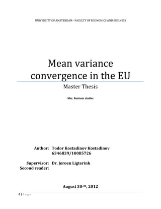
4.1 - H1: The historical mean variance characteristics
4.1.1 - H1.1: The historical mean variance characteristics in the old member states
0.00%
1.00%
2.00%
3.00%
4.00%
5.00%
6.00%
Jan-93
Aug-93
Mar-94
Oct-94
May-95
Dec-95
Jul-96
Feb-97
Sep-97
Apr-98
Nov-98
Jun-99
Jan-00
Aug-00
Mar-01
Oct-01
May-02
Dec-02
Jul-03
Feb-04
Sep-04
Apr-05
Nov-05
Jun-06
Jan-07
Aug-07
Mar-08
Oct-08
May-09
Dec-09
Jul-10
Mean variance distance USD old member states

32 | P a g e
Table 1.1 reports data on cross market level for the 16 countries in the OLD group for
each month during the period January 1993 to December 2010. Reported are the monthly mean
distance, variance distance and mean variance distance both in USD and in national currency.
Historically I measure that for this period the mean distance in USD(NAT) currency goes from
1.57% (1.40%) in the beginning of the period to 1.08% (0.97%) at the end of the period and is on
an average 1.15% (1.22%), the variance distance in USD (NAT) currency goes from 1.44%
(1.64%) to 0.95% (1.03%) and is on an average 1.17% (1.14%), the mean variance distance in
USD(NAT) currency goes down from 2.36% (2.34%) to 1.57%(1.55%) and is on an average
1.82% (1.85%). Graph 1.1 plots the historically measured evolution of the mean variance
distance in USD (NAT). As can be seen the evolution of the historical mean variance distance is
marked by two peaks around the late 90-ies and the 2008 financial crises. No significant time
trend is suggested from the graphics. The results from the ordinary least square regression I
calculate in USD(NAT) (13) also support this statement with a small negative beta coefficient of
the time variable -.0000064 (-.0000132) which is not statistically significant with P>|t| 0.418
(0.101). Poor F (1, 214) = 0.66 (2.72) also evidences that such model as a whole has no
statistically significant predictive capability.
Since I fail to reject the null hypothesis of no time trend, I conclude on my H.1.1 – the
historically measured mean variance distance exhibits no statistically significant time trend and
therefore the historical mean variance characteristics of the old EU member states have not
become more similar in real terms during the investigated period.

33 | P a g e
4.1.2 – H1.2: The historical mean variance characteristics in the new member states
Table 2.1 reports data on cross market level for the 5 countries in the NEW group for each
month during the period January 1999 to December 2010. I report monthly mean distance,
variance distance and mean variance distance both in USD and in national currency. The real
term historical measure I make for this period of the mean distance in USD(NAT) currency goes
from 2.76% (2.26%) to 0.84% (0.66%) and is on an average 1.62% (1.50%), the variance
distance in USD(NAT) currency goes from 2.42% (2.62%) to 0.31% (0.51%) and is on an
average 1.49% (1.39%), the mean variance distance in USD(NAT) currency goes from 4.21%
(3.94%) to 1.01% (0.87%) and is on an average 2.45% (2.27%). Graph 2.1 plots the historically
measured evolution of the mean variance distance in USD (NAT) and evidences an observable
time trend. The results from the ordinary least square regression (13) I calculate in USD (NAT)
also support this statement with a negative beta coefficient of the time variable -.0000693
(-.0000851) which is statistically significant with P>|t| 0.003 (0.000). Significant F (1,142) = 9.46
(15.98) also evidences that such model as a whole has a statistically significant predictive
capability. Predicted values of the regression estimated in Table 2.3 show that during the period
0.00%
1.00%
2.00%
3.00%
4.00%
5.00%
6.00%
7.00%
8.00% Jan-99
Jun-99
Nov-99
Apr-00
Sep-00
Feb-01
Jul-01
Dec-01
May-02
Oct-02
Mar-03
Aug-03
Jan-04
Jun-04
Nov-04
Apr-05
Sep-05
Feb-06
Jul-06
Dec-06
May-07
Oct-07
Mar-08
Aug-08
Jan-09
Jun-09
Nov-09
Apr-10
Sep-10
Mean variance distance USD new member states

34 | P a g e
the mean variance dissimilarities between the five new member states were reduced by 33.64%
and 42.21% in USD and national currency accordingly.
Since I reject the null hypothesis of no time trend, I conclude on my H.1.2 – the
historically measured mean variance distance exhibits a statistically significant time trend and
therefore the mean variance characteristics of the new EU member states have become more
similar in real terms during the investigated period.
4.2 – H2: The mean variance characteristics unlevered for volatility
4.2.1 – H2.1: The mean variance characteristics unlevered for volatility in the old member
states
Table 5.1 reports the mean variance distance on cross market level for the 16 countries in
the OLD group for each month during the period January 1993 to December 2010. Reported are
the monthly mean distance, variance distance and mean variance distance both in USD and in
national currency after unlevering for market volatility. I report that for this period the mean
distance in USD(NAT) currency goes down from 0.63%(0.60%) to 0.39%(0.40%) and is on an
average 0.47%(0.51%), the variance distance in USD(NAT) currency goes down from
0.58%(0.70%) to 0.34%(0.42%) and is on an average 0.45%(0.46%), the mean variance distance
in USD(NAT) currency goes down from 0.95%(1.01%) to 0.56%(0.64%) and is on an average
0.72%(0.77%). Graph 5.1 plots the historically measured evolution of the mean variance distance
in USD (NAT) and evidences for a slight observable time trend. The results from the preliminary
ordinary least square regression (13) I calculate in USD(NAT) also support this statement with a
small negative beta coefficient of the time variable -.000014187 (-.000015337) which is
statistically significant with P>|t| 0.000 (0.000). I report F (1, 214) = 44.62(52.01) which also
evidences that such model as a whole has a statistically significant predictive capability. These
preliminary results are the motive for the time trend investigation procedures I explained in
Section 3.1.6 and whose results follow below.

35 | P a g e
Next I report the results from the time trend investigation procedures. Table 5.4 and 5.5
show the results in USD and national currencies accordingly. Reported are data on overall cross-
market level as well as on national level. Following the Akaike Information Criterion (AIC) and
Schwarz' Bayesian Information Criterion (SBIC) I choose lag orders from 0 to 4 for each
investigated dependent variable. Second I report the Z (t) statistic from the Augmented Dickey
Fuller test, which for every investigated dependent variable is significantly smaller than its
critical value at 1% significance value. This rejects the null hypothesis of the test and essentially
implies that the error terms of the time series do not have a unit root, data is considered stationary
and regression results are not likely to be spurious. Next I move on to the results of the Newey
West heteroskedasticity and autocorrelation consistent regression. On overall cross market level
the beta coefficient is significantly negative when testing the convergence hypothesis for the
Euclidean mean variance distance as well as for its components the mean distance and the
variance distance. The results in USD and in national currencies are of similar magnitudes
implying that the exchange rates do not have a noticeable effect on the reported convergence
pattern. Thus I conclude that the mean variance characteristics of the OLD group of countries
have altogether become more similar during the investigated period once volatility is accounted
for. Both mean and variance dissimilarities have significantly decreased and together drive the
0.00%
0.20%
0.40%
0.60%
0.80%
1.00%
1.20%
1.40%
1.60%
1.80%
Jan-93
Aug-93
Mar-94
Oct-94
May-95
Dec-95
Jul-96
Feb-97
Sep-97
Apr-98
Nov-98
Jun-99
Jan-00
Aug-00
Mar-01
Oct-01
May-02
Dec-02
Jul-03
Feb-04
Sep-04
Apr-05
Nov-05
Jun-06
Jan-07
Aug-07
Mar-08
Oct-08
May-09
Dec-09
Jul-10
Mean variance distance unlevered for
volatility USD old member states

36 | P a g e
documented pattern of the Euclidean mean variance distance. As mentioned already I interpret
the intercept coefficient as the initial dissimilarity distance whereas the slope coefficient I
interpret as the speed of the diminishing dissimilarities. Projected values of the mean variance
distance in USD(NAT) show a 34% (35%) decrease over the investigated period which also
implies how much more similar have the stock markets of the old EU member become.
In the same table I also report results on national level as follows. The Euclidean mean
variance distance has decreased in all but two countries, namely Denmark and Ireland, where the
beta coefficients of the time variable are positive although insignificant both in USD. In national
currency only Denmark diverges albeit insignificantly. The rest of the countries exhibit
qualitatively similar results in USD and in national currencies with few exceptions. In dollar
terms eleven of the countries have significantly negative beta coefficients at the 10% level of
significance, namely Austria, Belgium, Finland, France, Germany, Greece, Italy, The
Netherlands, Portugal, Spain and Sweden. Cyprus, Luxembourg and The United Kingdom have
negative albeit insignificant beta coefficients. In national currency Austria still exhibits a negative
slope but with an insignificant P>|t|. On the other hand Luxembourg and The United Kingdom
show much more significantly negative slopes in national currencies. Once I look at the
components of the Euclidean distance I report that the mean similarities of both measured in USD
and in national currency show qualitatively similar behavior. The mean dissimilarities at the 10%
percent level of significance have decreased in Belgium, Cyprus, Finland, France, Germany,
Greece, Italy, Portugal, Spain and Sweden, whereas in Austria, Luxembourg, The Netherlands
and the United Kingdom they show insignificant negative trend. Ireland diverged albeit
insignificantly in terms of mean similarities. In national terms Luxembourg and The Netherlands
have much more significant results. The exchange rate does seem to affect the variance
similarities as Denmark and Ireland diverge in dollar terms and in domestic currency Denmark
and Cyprus diverge from the rest of the OLD member states. In dollar terms of the variance side
nine countries have significantly become more similar at the 10% level of significance, namely
Austria, Belgium, Finland, France, Germany, Greece, Italy, The Netherlands and Sweden. In
national currencies the results are similar except for Germany and Sweden showing insignificant
negative beta and Luxembourg showing significant negative beta at the 10% level of
significance.

37 | P a g e
Since I reject the null hypothesis of no time trend on cross market level as well as for the
majority of each separate country, I conclude on my H2.1 that the mean variance distance
unlevered for volatility has converged. Once accounted for volatility the stock markets of the 16
old EU member states seem much more similar in the mean variance space, precisely by 34%
(35%) in USD(NAT) as per the predicted values in the the Newey West heteroskedasticity and
autocorrelation consistent regression in Table 5.4 and 5.5.
4.2.2 – H2.2: The mean variance characteristics unlevered for volatility in the new
member states
Table 6.1 reports the distance estimates on cross market level for the 5 countries in the
NEW group for each month during the period January 1999 to December 2010. Reported are the
monthly mean distance, variance distance and mean variance distance both in USD and in
national currency after the effect of volatility has been taken out. I report that for this period the
mean distance in USD(NAT) currency goes from 0.68% (0.52%) to 0.35% (0.37%) and is on an
average 0.55% (0.56%), the variance distance in USD(NAT) currency goes from 0.60% (0.61%)
to 0.13% (0.28%) and is on an average 0.46% (0.47%), the mean variance distance in
USD(NAT) currency goes down from 1.04% (0.91%) to 0.42% (0.48%) and is on an average
0.00%
0.50%
1.00%
1.50%
2.00%
2.50%
Jan-99
Jun-99
Nov-99
Apr-00
Sep-00
Feb-01
Jul-01
Dec-01
May-02
Oct-02
Mar-03
Aug-03
Jan-04
Jun-04
Nov-04
Apr-05
Sep-05
Feb-06
Jul-06
Dec-06
May-07
Oct-07
Mar-08
Aug-08
Jan-09
Jun-09
Nov-09
Apr-10
Sep-10
Mean variance distance unlevered for
volatility USD new member states

38 | P a g e
0.79% (0.81%). Graph 6.1 plots the evolution of the mean variance distance unlevered from
volatility in USD (NAT) and evidences for a slight observable time trend. The results from the
preliminary ordinary least square regression (13) I calculate support the same statement as with
the levered mean variance distance negative beta coefficient of the time variable -0.000032 (-
0.000030) which is statistically significant with P>|t| 0.000 (0.000). I also report much more
significant F (1, 142) = 38.25 (33.79) which also evidences that such model as a whole has a
statistically stronger predictive capability.
In Tables 6.4 and 6.5 I report the results from the time trend investigation procedures in
USD and national currencies accordingly. Reported are data on overall cross-market level as well
as on national level. Following the Akaike Information Criterion (AIC) and Schwarz' Bayesian
Information Criterion (SBIC) I choose lag orders from 0 to 4 for each investigated dependent
variable. Second I report the Z (t) statistic from the Augmented Dickey Fuller test, which for
every investigated dependent variable is significantly smaller than its critical value at 1%
significance value. This rejects the null hypothesis of the test and essentially implies that the error
terms of the time series do not have a unit root, data is considered stationary and regression
results are not likely to be spurious. Next I move on to the results of the Newey West
heteroskedasticity and autocorrelation consistent regression. On overall cross market level the
beta coefficient is significantly negative when testing the convergence hypothesis for the
Euclidean risk return distance as well as for its components the mean distance and the variance
distance. The results in USD and in national currencies are of similar magnitudes implying that
the exchange rates do not have a noticeable effect on the reported convergence pattern. Thus I
conclude that the mean variance characteristics of the NEW group of countries have altogether
become more similar during the investigated period once volatility is accounted for. Both mean
and variance dissimilarities have significantly decreased and together drive the documented
pattern of the Euclidean risk return distance. Once plotted into a linear projection the data from
the Newey-West regression shows that the mean variance distance has decreased by 46.06%
(43.04%) which is also how much more similar the stock markets of the New EU member states
look in the mean variance space.
In the same tables I also report results on national level as follows. The Euclidean mean
variance distance has decreased significantly in all countries except Slovenia where the slope of

39 | P a g e
the time variable is still negative but insignificant. The rest of the countries exhibit qualitatively
similar results in USD and in national currencies. Looking at the components of the Euclidean
distance I report that the mean dissimilarities both measured in USD and in national currency
show a more significant convergence than the variance dissimilarities. The mean dissimilarities at
the 10% percent level of significance have decreased in The Czech republic, Hungary, Poland,
Poland and Romania, whereas in Slovenia they show insignificant negative trend. On the risk
side only The Czech republic and Romania have significantly become more similar at the 10%
level of significance a measured in USD. Slovenia also significantly converges in variance
distance in national currency at 10%. The rest of the countries show negative time trends
although insignificant.
I reject the null hypothesis of no time trend on cross market level as well as for the
majority of each separate country, and I thereby conclude on my H2.2 that the mean variance
distance unlevered for volatility has converged among the five new EU member states. Graph 6.2
illustrates the predicted values of the two country samples. As can be seen the negative slope of
the new members is much steeper and evidences for much faster convergence in comparison to
the old member states. In fact, projections show that immediately after 2008 crisis the new
member states outpaced the ones and are now closer to full convergence.

40 | P a g e
4.3 – H.3: The effect of volatility on the historical mean variance characteristics
4.3.1 – H3.1: The effect of volatility on the historical mean variance characteristics in the
old member states
Graph 3.1 plots the historically measured evolution of the mean variance distance in USD
(NAT) versus the historically measured market volatility as proxied by the average cross market
standard deviation of stock returns. The graphics suggest a positive linkage between volatility
and dissimilarity. Furthermore as can be seen at the graphics the end of the investigated period is
marked by higher level of volatility. If there is a positive relation between volatility and
dissimilarity, then volatility could be the reason for the lack of significant observable time trend
in the historically measured Euclidean risk return distance. I study this by looking at the
correlation matrix of cross market mean variance distance and the cross market volatility and as
can be seen in Table 3.1 I report high positive correlation coefficient 0.6553 (0.6644). I also
perform the ordinary least square regression (11) and report its results in Table 3.2 – positive
beta coefficient of the volatility variable in USD(NAT) .3707204 (.4080857) and statistical
significance with P>|t| 0.000(0.000). F (1, 214) = 161.05(169.09) also evidences that such model
as a whole has statistically significant predictive capability.
0.00%
2.00%
4.00%
6.00%
8.00%
10.00%
12.00%
Jan-93
Dec-93
Nov-94
Oct-95
Sep-96
Aug-97
Jul-98
Jun-99
May-00
Apr-01
Mar-02
Feb-03
Jan-04
Dec-04
Nov-05
Oct-06
Sep-07
Aug-08
Jul-09
Jun-10
Mean variance distance
USD
Market
volatility
USD

41 | P a g e
Since I report high positive correlation and also reject the null hypothesis of no
connection, I conclude on my H.3.1 that volatility exerted strong positive influence on the
historical mean variance distance and its higher levels at the end of the studied period may
explain the historical mean variance divergence in the stock market returns of the old EU member
states at the end of the investigated period.
4.3.2 – H3.2: The effect of volatility on the historical mean variance characteristics in the
new member states
Graph 4.1 plots the real term measures of the mean variance distance in USD (NAT)
versus the historically measured market volatility as proxied by the average cross market standard
deviation of stock returns among the new member states. As with the case of the mean variance
distance in the OLD group, a positive linkage between volatility and dissimilarity is present here
too even though the real historical risk return distance of the new member states actually
diminished over the studied period. The positive relation between volatility and dissimilarity
might have prevented a more significant observable time trend in the historically measured
Euclidean mean variance distance. I study this by looking at the correlation matrix of cross
market mean variance distance and the cross market volatility as can be seen in Table 4.1 where I
0.00%
2.00%
4.00%
6.00%
8.00%
10.00%
12.00%
14.00%
16.00%
Jan-99
Aug-99
Mar-00
Oct-00
May-01
Dec-01
Jul-02
Feb-03
Sep-03
Apr-04
Nov-04
Jun-05
Jan-06
Aug-06
Mar-07
Oct-07
May-08
Dec-08
Jul-09
Feb-10
Sep-10
USD
Volatility
USD

42 | P a g e
report correlation coefficient in USD(NAT) 0.704 (0.690). I also perform the ordinary least
square regression (11) and in Table 4.2 report a positive beta coefficient of the volatility variable
in USD(NAT) .5208981 (.5033682) which is statistically significant with P>|t| 0.000(0.000) and
F (1, 142) = 139.71 (129.42) evidencing that such model as a whole has statistically significant
predictive capability. By comparison the level of correlation with volatility here exceeds the one
in the OLD group by 7% (4%) and the slope coefficients of the (11) regression are 41% (23%)
steeper in USD(NAT). This comparison means that volatility has influenced more severely the
stock markets of the new member states.
Since I report high positive correlation and also reject the null hypothesis of no
connection, I conclude on my H.3.2 that volatility exerted strong positive influence on the
historical mean variance distance and its higher levels at the end of the studied period have
prevented the new EU member states from stronger historical mean variance convergence of their
stock market returns.
4.4 Channels of information for the mean variance convergence
In Table 7.1 I report the F (2, 428) values from testing the null hypothesis that each two
slope coefficients are equal. As can be seen the slope coefficients are overall different from each
other which leaves the door open for a research on a few possible explanations, namely testing
the H4.1-4. Tests performed and results reported in these sections (4.4.1 – 4.4.2) refer to the old
member states group only.
4.4.1 – H4.1: The initial distance and its effect on the speed of convergence
As reported in the previous section the mean variance convergence hypothesis is valid to
different extent with each different country. In this section I explain the results from a few
hypotheses I test for possible explanation. In Table 8.2 I first report that the initial distances and
the speeds of convergence reported in the previous section are highly negatively correlated both
in USD (NAT). For example in USD Finland and Greece with some of the highest intercepts of
0.01532447 and 0.01449293 also exhibit some of the most negative slopes,
namely (-0.000031995) and -0.000035334 accordingly. I therefore test the hypothesis that the
bigger the initial distance (intercept) the bigger the speed of convergence (more negative beta).
The results in Table 8.1 reject the null hypothesis with a negative beta coefficient of the initial

43 | P a g e
distance variable in USD (NAT)(-0.002774) (-0.002440) which is statistically significant at the
1%. I report F (1, 15) = 14.45(14.31) which evidences that such model as a whole has a
statistically significant predictive capability. Thus I conclude that in the investigated panel of the
16 countries during the period 1993 to 2010 the more different the national stock market was
initially, the faster it converged to average cross market levels of risk return similarity both in
USD and in national currency terms. Although I do not report it in this paper, I suspect that the
initial distance could also explain the relatively higher speed of convergence of the new members
versus the old ones.
4.4.2 – H4.2: The stock market size and its effect on the speed of convergence
Next I investigate whether and to what extent does the market capitalization of a national
stock market influences its convergence towards average cross market levels of risk and return. In
Table 9.2 I report a small negative correlation between the logarithm of the mean national stock
market capitalization in USD during the sample period and each market’s speed of convergence.
This suggests that the greater size of equity market cap of some of the studied countries may have
pushed them toward faster convergence in the mean variance space. Table 9.1 indeed reports a
negative beta coefficient of the slope variable -0.000170 but it is not statistically significant with
P>|t| 72.37%. I report F (1, 15) = 0.12 which evidences that such model as a whole lacks a
statistically significant predictive capability. Thus I conclude that in the investigated panel of the
16 countries during the period 1993 to 2010 the size of national stock market did not exhibit a
significant influence of the speed of convergence toward average cross market levels of risk and
return.
4.4.3 – H4.3: The long term trend in dividend yield dissimilarity on the speed of
convergence
Next I move on to the results from testing the hypotheses of Bekaert and Harvey (1995)
Table 10.1 reports data for the long term trends of dissimilarity in the dividend yields. I give data
on overall cross-market level as well as on national level all estimated in USD. I employ the 3-
step procedure from the risk return convergence hypothesis and report the calculated long term
trends. Following the Akaike Information Criterion (AIC) and Schwarz' Bayesian Information
Criterion (SBIC) I choose lag orders from 0 to 4 for each investigated dependent variable. Second

44 | P a g e
I report the Z (t) statistic from the Augmented Dickey Fuller test, which for every investigated
dependent variable is significantly smaller than its critical value at 1% significance value. This
rejects the null hypothesis of the test and essentially implies that the error terms of the time series
do not have a unit root, data is considered stationary and regression results are not likely to be
spurious. Next I perform the Newey West heteroskedasticity and autocorrelation consistent
regression and interpret each beta coefficient as the long term trend in each according
investigated variable. In light of the convergence dissimilarity hypothesis I expect negative trends
for each independent variable and hence positive connection to the negative slopes of the
unlevered risk return distance time regression. I report as follows.
Firstly in Table 10.1 I report that the long term trends in the dividend yield dissimilarity
are negative for most of the countries, which implies convergence in the dividend yields albeit
not statistically significant in all markets. In Table 10.3 I report a small negative correlation
coefficient with the speed of convergence of the unlevered mean variance distance, which is not
in line with expectations that stem from the Hypothesis of Bekaert and Harvey. I fail to reject the
null hypothesis of no positive connection between long term trend in the dividend yield
dissimilarity and speed of mean variance convergence. The results in Table 10.2 show a negative
beta coefficient of the long term trend of dividend yield similarity variable -0.01419 which is
statistically insignificant with P>|t| 0.74040. I report F (1, 15) = 0.11 which evidences that such
model as a whole has no statistically significant predictive capability. Thus I conclude that in the
investigated panel of the 16 countries during the period 1993 to 2010 the advance of dividend
yield similarity exerts no impact on the speed of convergence toward average cross market levels
of risk return similarity.
4.4.4 – H4.4: Negative volatility and its effect on the mean variance convergence
Finally in this section I report my results from testing the hypothesis that the Euclidean
mean variance distance converges asymmetrically depending on the stock markets being bearish
or bullish. Once I add the down dummy variable to the Newey West heteroskedasticity and
autocorrelation consistent regression I performed for H2 I report mixed evidence regarding the
effect of the bear market. For example in Table 11.1 which reports the USD regression, there are
both positive and negative significant slopes of the down dummy. In national currency the state
of the current market trend mostly does not exert a significant influence on the mean variance

45 | P a g e
distance. One notable exception here is Italy where both the time and the down variable are
significantly negative at the 1% level with F (2, 212) 47.37 and R2
= 0.3350. These results (11.2)
suggest that only in Italy the Euclidean risk return distance converged significantly faster during
times of bearish markets, which is not the case with the rest of the markets. Overall evidence
points to the rejection of H4.4 and to the conclusion that there is no asymmetry between bearish
and bullish market states.
4.5 – H5: Country versus industry effect on the mean variance characteristics after control
for volatility.
In this section I report my results from studying the country and industry effects on the
documented pattern of behavior of the unlevered Euclidean risk return distance. In Table 12.1 I
summarize the data collected from level 2 DATASTREAM stock market value indices. I average
the market value capitalization in USD of each country and industry over the studied period from
1993 to 2010 and present it as a percentage of the total market capitalization. As can be seen the
stock market capitalization of The United Kingdom accounts for nearly a third of the total market
with France, Germany, Italy and The Netherlands lagging far behind it with 17.75%, 14.19%,
7.87%, 7.11% total stock market capitalization share. The bulk of equity is concentrated in the
financial sector with 27.30% followed by Consumer services, Oil and gas, and Industrial sectors
with 10.00%, 9.73% and 9.36% accordingly. It can be said that the big markets such as The
United Kingdom, France and Germany are well diversified over the 10 industrial sectors while
the smaller national markets are rather concentrated in a couple of industries. For example
Austria, Belgium, Cyprus, Greece and Italy are specialized in the financial sector, whereas
Finnish market is entirely dominated by its technological sector, perhaps reflecting the presence
of the technological giant Nokia.
I recall that I use the methodology of Heston and Rouwenhorst (1994) and based on data
from level 2 Industrial composition of DATASTREAM I decompose (21) the level 1 National
stock market returns of the same information service. From the two new sets of returns each
reflecting industrial (22) and country (23) effects accordingly I calculate the Euclidean mean
variance distance and use the same 3-step time trend investigation procedures as in Section 3.1.5.

46 | P a g e
Firstly in Table 12.2 I summarize the two new sets of Euclidean mean variance distances
and their subcomponents the mean distance and the variance distance all unlevered for market
volatility. The most notable feature of the decomposed series is their magnitude difference. In
Table 12.2 I report that for this period the mean distance with country(industry) effect goes from
0.53% (0.005%) to 0.52% (0.004%) and is on an average 0.48% (0.01%), the variance distance
goes from 0.49% (0.01%) to 0.34% (0.00%) and is on an average 0.46% (0.01%), the mean
variance distance goes from 0.77% (0.01%) to 0.68% (0.01%) and is on an average 0.74%
(0.01%). The size difference between the two effects is in line with theory and it suggests that
any pattern of behavior of the country effect will exert much more influence on the behavior of
the Euclidean mean variance distance compared to the industry effect. The reported data are on
overall cross-market level measured in USD.
Next I move on to the time trend investigation procedures. Firstly I follow the Akaike
Information Criterion (AIC) and Schwarz' Bayesian Information Criterion (SBIC) and choose lag
orders from 0 to 4 for each investigated dependent variable. Second I report the Z (t) statistic
from the Augmented Dickey Fuller test, which for every investigated dependent variable is
significantly smaller than its critical value at 1% significance value. This rejects the null
0.00%
0.20%
0.40%
0.60%
0.80%
1.00%
1.20%
1.40%
1.60%
Jan-93
Dec-93
Nov-94
Oct-95
Sep-96
Aug-97
Jul-98
Jun-99
May-00
Apr-01
Mar-02
Feb-03
Jan-04
Dec-04
Nov-05
Oct-06
Sep-07
Aug-08
Jul-09
Jun-10
country effect
industry effect
Linear (Mean variance
distance country effect)

47 | P a g e
hypothesis of the test and essentially implies that the error terms of the time series do not have a
unit root, data is considered stationary and regression results are not likely to be spurious. Next I
move on to the results of the Newey West heteroskedasticity and autocorrelation consistent
regression. In Table 12.4 I report that the Euclidean mean variance distance in both industrial and
country effects shows a diminishing pattern of behavior, but this is much more evident in the case
of the country effect. The beta coefficient of the time variable with country effect is -0.0000144
compared to -0.0000006 and although they are both significant at the 1% level the former has
much better F (1, 214) and R-squared namely 40.43 and 0.18 compared to the same of the latter
namely F (1, 214) and R-squared of 14.31 and 0.06 accordingly.
From the reported magnitude of the country effect and its steeper slope when regressed on
the time variable I conclude that the documented pattern of mean variance convergence is
attributed to decreasing country effect and not industry effect. This is in line with the
expectations that stem from international financial market integration, where country specific
factors gradually become dominated by supranational market-wide factors. Graph 7.2 gives a
vivid illustration of the falling country effect in the mean variance dissimilarity.
4.6 – H6: The effect of the mean variance convergence on the investment opportunity set.
Based on data in Table 13.1.1 and 13.1.2 I report that for the period 1993-1998 (2005-
2010) the average mean variance distance unlevered for volatility is 0.78%(0.59%) whereas the
average correlation of returns is 0.47(0.82). This means that the two periods mark increasing
correlations and decreasing mean variance distances unlevered for volatility. To calculate the
Sharpe ratios and the efficient frontiers I take the mean weekly return of the 3-month US T-bill of
0.04%. Graph 8.1 shows an illustration of the three efficient frontiers. As can be seen both of the
hypothetical frontiers dominate the actual one which means that both increasing correlations and
decreasing mean variance distance exerted influence in the same negative direction. Furthermore
the second hypothetical efficient frontier lies above the first one with a Sharpe ratio of 0.41
compared to 0.33. This implies that during the studied period the increased mean variance
similarity exerted greater influence than the increased correlation of returns.

48 | P a g e
In Table 13.2.1 and 13.2.2 I report the correlation matrices of the returns in national stock
market indices in OLD and NEW group combined. I report that for the period 1999-2004 (2005-
2010) the average mean variance distance unlevered for volatility is 1.00% (0.78%) whereas the
average correlation of returns is 0.45 (0.77). As expected the two periods show increasing
correlations and decreasing mean variance distances. To calculate the Sharpe ratios and the
efficient frontiers I take the mean weekly return of the 3-month US T-bill of 0.04%. Graph 8.2
illustrates the three efficient frontiers. As with the hypothetical frontier reflecting the decreasing
mean variance difference in the OLD sample, here the same one dominates the other two. A
somewhat unexpected behavior I report with the frontier reflecting the increasing correlation of
returns. In theory it should have been located at least above the actual frontier, whereas in my
study it is the lowest of all three. I report the following Sharpe ratios for the actual, the first and
the second frontiers as 0.190, 0.186 and 0.195 accordingly. These results reconfirm the
observations from the OLD sample about the negative direction of the decreasing risk return
distance, but they are rather puzzling regarding the expected effect of the increasing correlation
of returns.
0.00%
0.10%
0.20%
0.30%
0.40%
0.50%
0.60%
0.70%
0.80%
0.00% 0.50% 1.00% 1.50% 2.00%
AverageReturn
Standard Deviation
Efficient Frontier in the old member states
Actual EF
Hypo II EF
Hypo I EF

Kostadinov.T._6346839._MSc.BS

Recommended

Recommended

More Related Content

Viewers also liked

Viewers also liked (15)

Similar to Kostadinov.T._6346839._MSc.BS

Similar to Kostadinov.T._6346839._MSc.BS (20)

Kostadinov.T._6346839._MSc.BS