2. 7. E. Betzig, J. K. Trautman, T. D. Harris, J. S. Weiner, and R. L. Kostelak, “Breaking the diffraction barrier:
optical microscopy on a nanometric scale,” Science 251(5000), 1468–1470 (1991).
8. K. Braeckmans, D. Vercauteren, J. Demeester, and S. C. De Smedt, “Nanoscopy and multidimensional optical
fluorescence microscopy,” in (Chapman and Hall, 2010).
9. H. Shroff, C. G. Galbraith, J. A. Galbraith, and E. Betzig, “Live-cell photoactivated localization microscopy of
nanoscale adhesion dynamics,” Nat. Methods 5(5), 417–423 (2008).
10. M. J. Rust, M. Bates, and X. Zhuang, “Sub-diffraction-limit imaging by stochastic optical reconstruction
microscopy (STORM),” Nat. Methods 3(10), 793–796 (2006).
11. S. T. Hess, T. P. K. Girirajan, and M. D. Mason, “Ultra-high resolution imaging by fluorescence photoactivation
localization microscopy,” Biophys. J. 91(11), 4258–4272 (2006).
12. N. Bobroff, “Position measurement with a resolution and noise-limited instrument,” Rev. Sci. Instrum. 57(6),
1152 (1986).
13. R. J. Ober, S. Ram, and E. S. Ward, “Localization accuracy in single-molecule microscopy,” Biophys. J. 86(2),
1185–1200 (2004).
14. L. A. Shepp and Y. Vardi, “Maximum likelihood reconstruction for emission tomography,” IEEE Trans. Med.
Imaging 1(2), 113–122 (1982).
15. A. Yildiz, J. N. Forkey, S. A. McKinney, T. Ha, Y. E. Goldman, and P. R. Selvin, “Myosin V walks hand-over-
hand: single fluorophore imaging with 1.5-nm localization,” Science 300(5628), 2061–2065 (2003).
16. M. P. Gordon, T. Ha, and P. R. Selvin, “Single-molecule high-resolution imaging with photobleaching,” Proc.
Natl. Acad. Sci. U.S.A. 101(17), 6462–6465 (2004).
17. R. E. Thompson, D. R. Larson, and W. W. Webb, “Precise nanometer localization analysis for individual
fluorescent probes,” Biophys. J. 82(5), 2775–2783 (2002).
18. R. Henriques, C. Griffiths, E. Hesper Rego, and M. M. Mhlanga, “PALM and STORM: unlocking live-cell
super-resolution,” Biopolymers 95(5), 322–331 (2011).
19. F. Huang, S. L. Schwartz, J. M. Byars, and K. A. Lidke, “Simultaneous multiple-emitter fitting for single
molecule super-resolution imaging,” Biomed. Opt. Express 2(5), 1377–1393 (2011).
20. A. Sergé, N. Bertaux, H. Rigneault, and D. Marguet, “Dynamic multiple-target tracing to probe spatiotemporal
cartography of cell membranes,” Nat. Methods 5(8), 687–694 (2008).
21. X. Qu, D. Wu, L. Mets, and N. Scherer, “Nanometer-localized multiple single-molecule fluorescence
microscopy,” in Proceedings of the National Academy of Sciences of the United States of America (2004), pp.
11298–11303.
22. E. A. Mukamel, H. Babcock, and X. Zhuang, “Statistical deconvolution for superresolution fluorescence
microscopy,” Biophys. J. 102(10), 2391–2400 (2012).
23. R. P. J. Nieuwenhuizen, K. A. Lidke, M. Bates, D. L. Puig, D. Grünwald, S. Stallinga, and B. Rieger,
“Measuring image resolution in optical nanoscopy,” Nat. Methods 10(6), 557–562 (2013).
24. J. L. Johnson and J. R. Taylor, “K-Factor Image Factorization,” in AeroSense’99. International Society for
Optics and Photonics (1999), Vol. 3715, pp. 166–174.
25. G. Pavlovic and A. Tekalp, “Restoration in the presence of multiplicative noise with application to scanned
photographic images,” Acoust. Speech. Signal 90, 1913–1916 (1990).
26. A. Toet, “Multiscale contrast enhancement with applications to image fusion,” Opt. Eng. 31(5), 1026 (1992).
27. J. L. Johnson and M. L. Padgett, “PCNN models and applications,” IEEE Trans. Neural Netw. 10(3), 480–498
(1999).
28. J. L. Johnson, M. L. Padgett, and W. A. Friday, “Multiscale image factorization,” Proc. Int. Conf. Neural
Networks 3, 1465–1468 (1997).
29. J. L. Johnson and J. R. Taylor, “Image factorization : a new hierarchical decomposition technique,” Opt. Eng.
38(9), 1517–1523 (1999).
30. R. Juskaitis, “Measuring the real point spread function of high numerical aperture microscope objective lense,”
in Handbook of Biological Confocal Microscopy, J. B. Pawley, ed. (Springer, 2006), pp. 239–250.
31. B. Zhang, J. Zerubia, and J. C. Olivo-Marin, “Gaussian approximations of fluorescence microscope point-spread
function models,” Appl. Opt. 46(10), 1819–1829 (2007).
32. J. R. Janesick, Scientific Charge Coupled Devices (SPIE Press monograph, 2001), pp. 605–419.
33. J. C. Waters, “Accuracy and precision in quantitative fluorescence microscopy,” J. Cell Biol. 185(7), 1135–1148
(2009).
34. M. K. Cheezum, W. F. Walker, and W. H. Guilford, “Quantitative comparison of algorithms for tracking single
fluorescent particles,” Biophys. J. 81(4), 2378–2388 (2001).
35. R. N. Ghosh and W. W. Webb, “Automated detection and tracking of individual and clustered cell surface low
density lipoprotein receptor molecules,” Biophys. J. 66(5), 1301–1318 (1994).
36. D. L. Snyder, C. W. Helstrom, A. D. Lanterman, M. Faisal, and R. L. White, “Compensation for readout noise in
CCD images,” J. Opt. Soc. Am. A. 12(2), 272–283 (1995).
37. M. D. Abràmoff, J. M. Paulo, and J. R. Sunanda, “Image processing with ImageJ,” Biophotonics Int. 11, 36–42
(2004).
38. R. Henriques, M. Lelek, E. F. Fornasiero, F. Valtorta, C. Zimmer, and M. M. Mhlanga, “QuickPALM: 3D real-
time photoactivation nanoscopy image processing in ImageJ,” Nat. Methods 7(5), 339–340 (2010).
39. N. Banterle, K. H. Bui, E. A. Lemke, and M. Beck, “Fourier ring correlation as a resolution criterion for super-
resolution microscopy,” J. Struct. Biol. 183(3), 363–367 (2013).
#198546 - $15.00 USD Received 30 Sep 2013; revised 20 Nov 2013; accepted 21 Nov 2013; published 16 Dec 2013
(C) 2013 OSA 1 January 2014 | Vol. 5, No. 1 | DOI:10.1364/BOE.5.000244 | BIOMEDICAL OPTICS EXPRESS 245
3. 1. Introduction
Fluorescence microscopy is the most popular technique used in biological imaging
applications [1,2] due to the capabilities to target and modify specific single proteins within
the host organism. However, the resolution of a visible light microscope is limited by the
phenomenon of diffraction [3] to length scales set by the Rayleigh criterion to approximately
half the wavelength of the light [4,5]. Due to this limitation, any object smaller than the
microscope resolution will appear as a diffraction-limited spot with a point spread function
(PSF) given by an Airy function. The desire to observe biological structures and functions at
length scales smaller than the diffraction limit has led to the development of super-resolution
techniques that enable imaging intracellular structures with sub-diffraction-limit accuracy [6–
8].
Single molecule localization microscopy techniques, such as PALM [9] and STORM [10],
use optical control to activate a sparse subset of fluorescently tagged proteins in which the
PSF of each individual activated fluorophore does not overlap with that of its nearest
activated neighbor. This allows for the determination of the position of individual probes to a
much higher accuracy than conventional optical methods. The cycle of activation, imaging,
and photobleaching is repeated until all the fluorophores are exhausted, or a sufficient number
of them have been localized, and the measured molecular positions are then plotted to
generate a composite image [11].
In super-resolution microscopy, ultraprecise localization is usually accomplished by
fitting the diffraction-limited image of individual fluorophores to an ideal PSF using
algorithms such as non-linear least squares [12,13], and maximum likelihood [14]. These
methods can provide precision down to ~10nm, limited primarily by the number of photons
collected from each particular fluorophore [15,16], and have been used to great effect in
single particle tracking as well as in other imaging related applications. In these techniques,
reliable localization of a single fluorescent molecule requires both a sufficient number of
photons (N) in the measured PSF, and that the activated molecules be spatially separated by a
distance greater than several times the width of their PSFs [17]. Overlapping PSFs in standard
localization algorithms are generally discarded; this requires that the activation density remain
low across the field of view, which increases the composite image acquisition time [18]. To
address this problem, several methods have been recently developed with the aim of
localizing overlapping PSFs. One utilizes a maximum likelihood technique with increasing
numbers of point sources within the recorded PSF in the localization algorithm and is built for
graphics processing unit (GPU) analysis, and as such is relatively fast – the analysis time is
on the order of minutes [19–21]. Another paper uses a statistical deconvolution technique that
iterates through the observed PSF with a guess-work of overlapping PSFs. This approach is
very slow and requires ~10 times more computation time/frame than the other methods of
single-emitter fitting [22].
The problem of overlapping PSFs in super-resolution microscopy also affects the ultimate
spatial resolution of the composite image. In particular, the achievable spatial resolution is
determined by the localization density (i.e., the density of successfully localized spots) in
addition to the precision of each localization [17,18,23]. Using conventional localization
algorithms, when the number of photons emitted by the fluorophore is relatively low or the
spots are closely spaced, the localization density decreases since many regions of interest
(ROI: areas on the image that map to actual fluorophore locations on the sample) are
discarded in the analysis. Thus, high localization precision, high labeling density, and near-
unity localization efficiency of those fluorescent labels are all needed to achieve the best
possible spatial resolution. Here, we demonstrate a nonlinear image-factorization algorithm
designed for two distinct but related purposes: to suppress image noise associated with low
signal levels (poor photon statistics) and to differentiate image features associated with
different contrast levels. This approach increases spatial resolution and image acquisition
#198546 - $15.00 USD Received 30 Sep 2013; revised 20 Nov 2013; accepted 21 Nov 2013; published 16 Dec 2013
(C) 2013 OSA 1 January 2014 | Vol. 5, No. 1 | DOI:10.1364/BOE.5.000244 | BIOMEDICAL OPTICS EXPRESS 246
4. speed both by requiring fewer photons to achieve the same localization precision and by
allowing for a higher density of activated fluorophores during each acquisition cycle.
The aim of this algorithm is effectively to sharpen the edges of the PSF from a single
point source. This sharpening will simultaneously allow isolated fluorophores to be localized
with higher precision (for a given number of photons), and two overlapping fluorophores to
be effectively isolated such that each can be localized to high precision. Usually, spatial
denoising techniques can be divided into linear and nonlinear approaches [24]. Mean and
Wiener filters [25] are two classical linear solutions which simply mask an image using the
local statistical measurements of pixels. At the same time, they also blur the edge. On the
contrary, nonlinear filtering technologies have the advantages to preserve the edge and fine
details. One such method is a multiscale renormalization algorithm which produces a fused
image by nonlinear recombination of the ratio of low-pass (ROLP) pyramidal decompositions
of the original images [26]. Another method is a cyclic algorithm for shadow removal based
on pulse-coupled neural networks (PCNN), an image processing algorithm derived from
biologically-grounded cortical models that addressed the experimental findings of stimulus-
induced synchronous bursts of pulse activity [27,28]. The PCNN-based factorization is an
efficient image-processing tool for noise smoothing and elementary image segmentation that
operates on local image patches. However, these methods are mathematically intractable and
have a high computational complexity. The adopted method is a non-linear algorithm, which
improves contrast at the PSF edges without increasing spurious noise. In particular, our
method uses the K-factor transformation, which decomposes the image into hierarchical
contrast-ordered factors whose joint product reconstructs the original pattern [29]. The K-
factor decomposition divides the image pattern into factors where noise elements are distinct
from those containing the image structure of interest. In this decomposition, the first few
components, which have the highest contrast depth, contain mainly the desired image
information while the higher orders contain mostly noise components. The K-factor algorithm
is applied to raw image data prior to emitter localization, and does not add much
computational complexity nor processing time, requiring only fractions of a millisecond per
frame. Furthermore, the proposed method reduces the total number of individual frames that
are required for the reconstruction of the final image, thus reducing the overall computation
time.
The paper is organized as follows: First, the theoretical background for imaging single
molecules, the mathematical background for nonlinear filtering algorithms, and the K-factor
transform are presented. Second, numerical simulations for a variety of parameters inherent in
the K-factor algorithm are presented and fully discussed. Third, the proposed algorithm is
applied on experimentally acquired images to validate the approach.
2. Theoretical background
For an aberration-free imaging system, the diffraction-limited point spread function
corresponding to a single point emitter (i.e. fluorescent label) is given by an Airy function
[30]. Near the peak, this function is approximated by a Gaussian, which is mathematically
simpler [31]. The measured intensity of the diffraction limited spot is given by the acquired
data together with photon shot-noise, background noise created most commonly by out-of-
focus fluorescence, charge coupled device (CCD) readout noise, dark current, and extraneous
fluorescence in the microscope. The model for the intensity at (x,y) of a fluorescent particle
located at (x0,y0), is given by [17]:
2 2
0 0
2
x x y y
2σ
B shot2
N
I x,y e η η
2πσ
(1)
where N is the total number of photons collected from the fluorophores' label by the image
acquisition system during the measurement period, σ is the standard deviation of the
#198546 - $15.00 USD Received 30 Sep 2013; revised 20 Nov 2013; accepted 21 Nov 2013; published 16 Dec 2013
(C) 2013 OSA 1 January 2014 | Vol. 5, No. 1 | DOI:10.1364/BOE.5.000244 | BIOMEDICAL OPTICS EXPRESS 247
5. Gaussian, that is given by setting the e1
point of the intensity model to be equal to the
Rayleigh radius, ηB is a Poisson distributed random variable with variance Nb that describes
the background noise (assumed constant across the field of view), and ηshot is a Poisson
distributed random variable that describes the shot noise with a mean equal to the square root
of the total intensity in each pixel [32]. In the absence of aberrations, the values will be equal
and given by [33]:
0.6 λ
σ
2N.A.
(2)
where N. A. is the numerical aperture of the objective and λ is the wavelength of the emitted
light.
In existing localization microscopy methods, the assumption is that two fluorophores must
be spatially well separated to achieve minimal penetration of the tails of one PSF into the
other. The detection of each PSF is accomplished by establishing an intensity threshold value
that distinguishes background from signal and determining whether a certain PSF exceeds this
value. If so, the data is fit to a model of a Gaussian profile with a single peak. If the two PSFs
are in close proximity such that the saddle between them is higher than the threshold, they
will be indistinguishable and be considered as one, resulting in an increased localization error.
To mitigate these errors, ROIs exhibiting elongated (asymmetric) intensity profiles are often
discarded from the sample set, effectively reducing the sampling density. Thus, the ability to
reduce the saddle between two overlapping PSFs will allow for fewer discarded point sources
in the localization algorithm, while also allowing for faster data acquisition rates.
3. K-factor algorithm
The K-factor algorithm is an image factorization [24,29] technique, which reduces an image
into a nonlinear finite or infinite set of contrast-ordered pseudoimage factors whose joint
product reassembles the original image.
The K-factor transformation of an image I(x,y) can be described mathematically as:
n
n 1
I x,y f x,y
M
(3)
where M is the number of factors that reconstruct the image, and fn are the pseudo image
factors that when multiplied together reconstruct the image and are given by:
n1 k g x, y
nf x, y
n n1 k
(4)
where the parameter k controls the contrast depth at each level with a value is between 0 and
1, and gn is a binary image computed as:
n 1 n
jj 1
I x, y 1
1
1 k, f x, y
0 .
ng x y
OW
(5)
The factorization algorithm is an iterative process that is based entirely on the depth of
contrast. The choice of k orders the image into different contrast depth factors. A small value,
close to zero, will give large contrast steps and produce a spatially coarse version of the image
with relatively few factors, while a value close to unity produces an image version with fine
geometrical details with a larger amount of factors.
#198546 - $15.00 USD Received 30 Sep 2013; revised 20 Nov 2013; accepted 21 Nov 2013; published 16 Dec 2013
(C) 2013 OSA 1 January 2014 | Vol. 5, No. 1 | DOI:10.1364/BOE.5.000244 | BIOMEDICAL OPTICS EXPRESS 248
6. For each n, the function gn that represents each pixel in the image is set to be either 1 or 0
according the threshold set by k. This will set the value for the factor fn. The original image is
then divided by the factor fn and this sets the threshold for the next iteration of gn. As a result,
the first few factors exhibit the largest depth of contrast, and mostly contain the desired image
information along with details related to image distortion. Since the desired image
information and distortion details generally exhibit different contrast levels, they typically
separate into distinct factors, allowing for their differentiation. Random spatial noise usually
falls into the higher-order factors, due to their lower contrast levels.
The K-factor algorithm produces a set of contrast-ordered factors, which when multiplied
together according to Eq. (3) will reproduce the original image with high fidelity, provided
appropriate values of k and M. If, however, the running product is truncated at a lower-order
factor fh, where h<M, then those image components with lower contrast levels (i.e., mostly
noise) will be de-emphasized in the reconstruction. In addition to noise, the truncated high
order factors might also contain some fine spatial information associated with low contrast
levels. Thus, we multiply the truncated product by the original image to restore some of these
fine spatial details:
1
, , ,
h M
h n
n
R x y I x y f x y
(6)
where Rh(x,y) is the truncated reconstruction. The optimal choice of the parameters k and M,
as well as the number of factors h in the truncated reconstruction, depends entirely on the
nature of the image, rather than on a pre-chosen spatial scale, and therefore it is determined de
novo for each application.
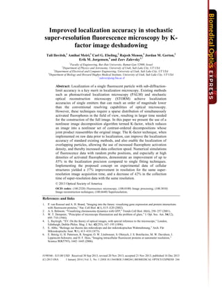
Figure 1 illustrates the influence of the K-factor transform on a noiseless image containing
two PSFs separated by a distance of 3σ~600nm. The K-factor parameters are k = 0.9, M = 48,
h = 8. It is clearly seen that the overlap between the two PSFs was reduced.
Fig. 1. Image of two PSFs separated by a distance of 3σ~600nm . Before the K-factor
transform (black) and after the K-factor transform (red).
The proposed technique is an added step during the conventional PALM routine as
illustrated in Fig. 2(b). The suggested super-resolved image acquisition technique begins with
single frame acquisition using repeated cycles of activation and imaging of the activated
fluorophores followed by bleaching to minimize the presence of already visualized particles
in posterior acquired images. The frame is passed on to a computer program like MATLAB
software package (MathWorks, Natick, MA, USA), where it is applied with the K-factor
#198546 - $15.00 USD Received 30 Sep 2013; revised 20 Nov 2013; accepted 21 Nov 2013; published 16 Dec 2013
(C) 2013 OSA 1 January 2014 | Vol. 5, No. 1 | DOI:10.1364/BOE.5.000244 | BIOMEDICAL OPTICS EXPRESS 249
7. algorithm. The next step is the localization of the activated fluorophores using methods of
single emitter fitting. Reconstruction and creation of the super-resolved image is done by
summing the molecular images across all frames.
Fig. 2. Super-resolution image acquisition steps for conventional PALM (a) and acquisition
steps for the K-factor algorithm (b). Conventional PALM acquisition is divided into three
independent steps: frame acquisition using repeated cycles of activation and imaging of the
activated fluorophores followed by bleaching to minimize the presence of already visualized
particles in posterior acquired images. Localization of the activated fluorophores using
methods of single emitter fitting. Reconstruction and creation of the super-resolved image by
summing the molecular images across all frames. The K-factor analysis adds a step prior to the
localization and is applied to each frame using computer software.
4. Simulation results
To evaluate the performance of the K-factor transformation routine and its impact on
localization precision, Monte-Carlo simulations were used to generate mock data sets with
two emitters in each set. In these simulations the model was a fluorescence source with λ =
540nm that was imaged through an objective lens onto a CCD camera. The model matches
the parameter of the Zeiss Axiovert 200 microscope using a 63x objective, 1.2N.A. water
immersion objective lens. Each pixel on the CCD sensor array had dimensions of 6.45μm ×
6.45μm, which translates to 102nm × 102nm in the image plane with the 63x objective.
Background noise was introduced by adding a sample from a Poisson distribution with the
parameter Nb. Shot noise was introduced by adding a Poisson distribution with parameter that
is the square root of the total intensity of the light at each pixel. The value for σ in the model
used for the PSF was calculated from Eq. (2) to be 191nm for the given imaging parameters.
Gaussian fitting was performed on both the raw simulated data and K-factor filtered data.
Each image contained a randomly positioned fluorophore, which was fit using the non linear
least-squares minimization routine lsqnonlin in MATLAB to fit a model of the form of:
2 2
0 0
2
x x y y
2σ
psf 2
N
I x, y e
2πσ
(7)
where N,σ, x0 and y0 are all fit parameters. The algorithm initially detected the position of
each particle as the pixel with the highest intensity in its region, and preformed a fit by taking
9 × 9 pixels around this initial location [34]. The fit produces the best estimate of the position
of that particular fluorophore, and the process is repeated many times yielding a set of L
localization positions xi, i) that can be compared with the known positions (xi,yi). The root
mean square (RMS) localization error is computed for both the raw and K-factor filtered
simulated data:
#198546 - $15.00 USD Received 30 Sep 2013; revised 20 Nov 2013; accepted 21 Nov 2013; published 16 Dec 2013
(C) 2013 OSA 1 January 2014 | Vol. 5, No. 1 | DOI:10.1364/BOE.5.000244 | BIOMEDICAL OPTICS EXPRESS 250
8.
2 2
1
1 L
rms i i i i
i
yerr x x y
L
(8)
The position of the each fluorophore, the distance between fluorophores, the number of
arriving photons N, the background noise parameter Nb, the K-factor parameter k and the
number of harmonics h, were allowed to vary. All analysis was performed in MATLAB.
A crucial aspect is the choice of the parameter k, and thus it was carefully determined after
numerous simulations and iterations, to result in a reliable decomposition of the image. The
simulated image contained two PSFs separated by 3σ~600nm. The k parameter varied
between 0-1. Additional noise was not introduced in order to reach maximum correlation and
maximize the k parameter. For each k value, the maximum correlation between the
reconstructed image and the original image was calculated using the corr function in
MATLAB (as shown in Fig. 3 (left y axis)), and also the number of factors needed for
achieving maximum correlation (as shown in Fig. 3 (right y axis)).
Fig. 3. Maximum correlation between the reconstructed image and the original image of two
PSFs separated by a distance of 3σ~600nm, as a function of k values (left y axis). Number of
factors needed for maximum correlation as a function of k values (right y axis).
It is clearly seen that for lower k values, the correlation is less than 75%, and therefore the
residual error is relatively large, whereas for higher k values, the correlation can reach 100%,
which means full reconstruction. A value of only k = 0.9 yielded a correlation of 100%; thus
a higher k value would not additionally contribute to image reconstruction. It is also evident
that the higher the k value, the more factors are required for the full reconstruction, as is
predicted by theory, and full image reconstruction results in a longer computation time. Due
to this tradeoff between correlation and the overall number of factors, users with
computational considerations can choose to work with a lower image correlation, for example
a correlation of 95%, with k = 0.5, where the number of factors is only 10. This will result in
a smaller improvement in resolution in the reconstructed image when compared to using a
value of k = 0.9.
Another key merit is the number of harmonics that the reconstructed image is multiplied
by, and its effect on the overlapping of neighboring PSFs. The first factors in the
decomposition contain most of the signal’s information, where the higher-order factors
contain mostly the noise. By multiplying the data with the first harmonics that contain most of
the signal data, the signal intensity increases and can be discriminated from the noise.
Simulations were carried in order to find the number of harmonics that contain only the signal
for different k values. Empirically, the formula that describes the number of harmonics that
contains only the signal:
1
6
h n (9)
#198546 - $15.00 USD Received 30 Sep 2013; revised 20 Nov 2013; accepted 21 Nov 2013; published 16 Dec 2013
(C) 2013 OSA 1 January 2014 | Vol. 5, No. 1 | DOI:10.1364/BOE.5.000244 | BIOMEDICAL OPTICS EXPRESS 251
9. where n is the number of factors needed for achieving a correlation of 100% with the original
image prior to the decomposition, for a given k. Figure 4(b) presents the influence of the
number of multiplied harmonics on the RMS error in localization as a function of distances
between centers for k = 0.9, n = 48. The lowest RMS error was obtained for h = 8 calculated
according to Eq. (9). The signal information contained in these h = 8 factors equals 91% of
the entire signal information. A lower value of h results in a reduced impact of the algorithm,
since not all the signal components were enhanced. For the end case of h = 0, the
reconstructed image equals the original image and the error equals the predicted value for the
least squares algorithm [17]. Increasing h also decreases the effect, since both the signal and
the noise were enhanced, and the algorithm's influence becomes negligible. For the end case
of h = n, the error returned is the same as for h = 0.
Figure 4(a) illustrates the relation of the K-factor transform and h on overlapping PSFs
according to Eq. (9) for a relatively low k = 0.4 (red) and for high k = 0.9 (blue). In such a
scenario, the PSF degradation is due to the overlap of the PSFs with each other, and in order
to present the influence of the algorithm on closely spaced PSFs, no additional noise was
added. The saddle was reduced by 56.1% and 54.2% respectively. However, the lower k
distorts the image and reduces the effect of improved localization.
Fig. 4. (a) The K-factor effect on overlapping PSFs for k = 0.4 (red) and k = 0.9 (blue). (b) the
influence of the number of multiplied harmonics on the RMS error in localization as a function
of distances between centers for k = 0.9, n = 48.
The shot noise is a Poisson random process with rate that depends on the total number of
photons detected. It is proportional to N, as can be seen in Fig. 5, e.g. an increased number
of emitted photons results in a more accurate localization precision [35]. Figure 5 compares
the results of the least squares fitting process applied to raw data (black line) and applied to
raw data that underwent processing with the K-factor algorithm (red line). It is clearly seen
that applying the K-factor algorithm on the raw data followed by the least squares fitting
process, resulted in localization error of ~3.5nm for a high photon count and for a distance of
3σ, an error that is lower than the predicted localization accuracy for the least squares
algorithm by itself [17]. The reason for this is due to the influence of the algorithm on the
reduction of the σ of each PSF. It narrows the width of the PSF, while allowing for the
isolation and localization of overlapping PSFs. For example, in Fig. 4(a), applying the K-
factor technique yielded a reduction in σ, by a factor of 1.5, which results in a localization
RMS error that is lower than N.
#198546 - $15.00 USD Received 30 Sep 2013; revised 20 Nov 2013; accepted 21 Nov 2013; published 16 Dec 2013
(C) 2013 OSA 1 January 2014 | Vol. 5, No. 1 | DOI:10.1364/BOE.5.000244 | BIOMEDICAL OPTICS EXPRESS 252
10. Fig. 5. Error in localization as a function of detected photons, distance between particles 3σ
~600nm, without background noise. The simulation contained 1000 Monte-Carlo iterations.
The background noise variance for each pixel is a parameter, marked by Nb, that can be
measured experimentally and therefore is considered to be known [36], and varied in our
simulations between 0 to 10 photons. We calculated the improvement (%) in localization
error according to:
100
original K Factor
original
RMS RMS
Improvement
RMS
(10)
The results can be seen in Fig. 6. For a distance of 3σ ~600nm), at low Nb of 0-2 photons, the
improvement was 40-50%, and with the background increased up to Nb = 10 photons, the
improvement reaches up to 85%. For low photon counts, the improvement in localization
accuracy is the most pronounced, and for fluorophores with lower photon yields, such as
fluorescent proteins, this will produce the most dramatic improvements in localization
accuracy. Since our proposed technique is aimed for reducing noises, the higher the
background noise is, the higher the improvement in localization over existing methods. The
improvement is achieved due to the high noise discrimination capabilities of the deshadowing
algorithm.
#198546 - $15.00 USD Received 30 Sep 2013; revised 20 Nov 2013; accepted 21 Nov 2013; published 16 Dec 2013
(C) 2013 OSA 1 January 2014 | Vol. 5, No. 1 | DOI:10.1364/BOE.5.000244 | BIOMEDICAL OPTICS EXPRESS 253
11. Fig. 6. The improvement in detection using the K-factor algorithm as a function of detected
photons, for different background noise photons Nb. The distance between particles was 3σ
~600nm.
As can be seen in Fig. 7, without background noise, at close distances of 2.5-4.σ and with
a low photon count, the improvement in detection of each spot can reach up to 85%. At larger
distances, the obtained improvement is reduced to ~5-20%, depending on the photon count.
Fig. 7. The improvement in localization using the K-factor algorithm as a function of the
distance between florescence centers for different number of photons N, without background
noise and with k = 0.9, h = 8.
5. Experimental results
Single molecule imaging experiments were performed in an epi-fluorescence microscope
setup consisting of an inverted microscope (Zeiss Elyra P.1, Carl Zeiss Microscopy Inc.), 1.46
N.A. total internal reflection (TIRF) objective, 642nm diode laser, and an electron multiplying
CCD camera Ixon (897, Andor Technologies PLC.) with EM gain set to 200. The epi-
fluorescence filter setup consisted of a dichroic mirror (650nm, Semrock) and an emission
filter (692/40, Semrock). The sample chamber was mounted in a 3D piezostage (P-737
PIFOC Specimen-Focusing Z Stage, Physik Instrumente). 10,000 images were taken in a
TIRF configuration at 40frames/second. Frames were 512 × 512 pixels with an effective pixel
#198546 - $15.00 USD Received 30 Sep 2013; revised 20 Nov 2013; accepted 21 Nov 2013; published 16 Dec 2013
(C) 2013 OSA 1 January 2014 | Vol. 5, No. 1 | DOI:10.1364/BOE.5.000244 | BIOMEDICAL OPTICS EXPRESS 254
12. size of 99.8nm. The K-factor technique was tested experimentally by imaging microtubules
from BSC-1 African green monkey kidney epithelial cells (American Type Culture
Collection-ATCC). These cells were cultured and stained with Alexa 647 phalloidin
fluorescent probes, using Abcam rat antibody to tubulin, ab6160 as the primary antibody, and
Invitrogen Alexa Fluor® 647 Goat Anti-Rat, A-21247 as the secondary antibody. Cell culture
methods were standard cell culture techniques for primary/secondary antibody labeling
methods. The peak emission wavelength of Alexa 647 is 671nm. Image pre-processing of the
raw data that contained noise filtering and application of the K-factor algorithm on each
frame was performed using MATLAB. The localization and the reconstruction of the super-
resolved image was done in ImageJ [37] using QuickPALM plugin [38].
The fluorescence data included individual frames in which pairs or larger groups of
fluorophores were simultaneously activated and produced a data set with overlapping
molecules (Fig. 8(a)). The reconstruction of the final super-resolution PALM image was
achieved using extracted data from 10,000 frames. The K-factor method was performed on
each of the 10,000 individual frames followed by the same localization and reconstruction
procedures to construct a super-resolution image. By applying the K-factor algorithm on each
individual frame (Fig. 8(b)), areas with overlapping molecules became distinguishable (Figs.
8(d), 8(f), 8(h)) compared to the original image (Figs. 8(c), 8(e), 8(g)).
Fig. 8. Individual PALM frame without processing (a) and after K-factor processing(b).
Marked regions is where the difference can be clearly seen. (c),(e) and (g) is the magnification
of the marked areas in (a). (d),(f) and (h) is the magnification of the marked areas in (b).
The proposed method's performance was tested as follows: first a conventional PALM
analysis was performed on the data (Fig. 9(a)), in which frames that contained overlapping
emitters were localized (Fig. 9(b)). Subsequently, the K-factor algorithm with parameters of k
= 0.9, n = 48, was applied to the data (Fig. 9(d)) followed by the same single molecule fitting
technique (Fig. 9(e)). As can be seen from the fitting process using both the conventional
#198546 - $15.00 USD Received 30 Sep 2013; revised 20 Nov 2013; accepted 21 Nov 2013; published 16 Dec 2013
(C) 2013 OSA 1 January 2014 | Vol. 5, No. 1 | DOI:10.1364/BOE.5.000244 | BIOMEDICAL OPTICS EXPRESS 255
13. PALM and the K-factor algorithm in (Fig. 9(b) and 9(e)), when neighboring molecules were
in close proximity, like in the upper section of the image, the K-factor routine enabled the
identification of two overlapping molecules, whereas in its absence, only one molecule was
identified. Figure 9(c) and 9(f) show the cross section of the dashed line that passes through
the center of the overlapping two emitters with σ = 195nm in the upper part of the image of
Fig. 9(b) and 9(e) respectively. As can be seen, applying the proposed method prior to the
localization reduces the saddle of overlapping PSFs and enables their localization.
Fig. 9. Single molecule fitting process preformed on individual frames of conventional PALM
(Upper row) and on frames preprocessed by the K-factor algorithm (Lower row). (b) is the
magnification of the marked area in (a). PALM analysis (blue circles) localize 2 emitters. (e) is
the magnification of the marked area in (d). K-factor preprocessing followed by PALM
analysis (red crosses) localize 3 emitters. (c) and (f) show the cross section of the dashed line
that passes through the center of the overlapping two emitters with σ = 195nm in the upper part
of the image in (b) and (e) respectively.
In order to create the fully reconstructed image, all the single emitter estimations of
individual frames were summed, using both the unprocessed images and the K-factor
processed images. The use of the K-factor algorithm enabled the extraction of data that
otherwise would have been discarded from each frame, which resulted in the ability to
reconstruct the full image with fewer frames than the conventional PALM image. To quantify
the reduction in number of frames that require the full reconstruction using the K-factor
process, an iterative approach was used. First, the correlation coefficient between the two
images was calculated for a total number of 10,000 frames used for the reconstruction. Then,
for this given correlation coefficient, the number of frames in the K-factor reconstruction
process was reduced, until the point where the correlation coefficient decreased by 5%. This
was set to be the lowest number of frames needed for the full reconstruction in comparison to
the conventional PALM.
Using the K-factor algorithm, only 5,735 frames were required for the full reconstruction
of the image (Fig. 10(b)) whereas conventional PALM analysis required 10,000 (Fig. 10(c)).
Taking only 5,735 frames using the conventional PALM produced a less detailed image
estimation with gaps in locations where there was a high density of overlapping emitters (Fig.
10(a)). Taking 10,000 frames using the K-factor algorithm resulted in a sharper image
estimate, due to the higher accuracy in localization (Fig. 10(d)).
#198546 - $15.00 USD Received 30 Sep 2013; revised 20 Nov 2013; accepted 21 Nov 2013; published 16 Dec 2013
(C) 2013 OSA 1 January 2014 | Vol. 5, No. 1 | DOI:10.1364/BOE.5.000244 | BIOMEDICAL OPTICS EXPRESS 256
14. Fig. 10. Reconstruction of imaging data from Alexa647 labeled microtubules sample without
processing and using the K-factor algorithm prior to the localization. Images in the upper row
represent reconstructed image using 5,735 frames and those in the lower row represent
reconstructed image using 10,000 frames. (a,c) conventional PALM analysis. (b,d) K-factor
algorithm applied to raw data followed by conventional PALM analysis.
The effective resolution of the reconstructed image was measured using the method of
Fourier ring correlation (FRC) [23,39]. FRC evaluates the degree of correlation of two
independent reconstructions of the same object in frequency space and determines the
resolution threshold (the spatial frequency) at which both reconstructions are consistent and
considered to be resolved. Reconstruction using 10,000 individual frames without additional
processing resulted in effective resolution of 55.74nm, whereas taking the same amount of
frames and using the K-factor algorithm additional processing yielded a resolution of
43.21nm. When taking only 5,735 frames, the resolution obtained without additional
processing was 80.16nm, compared to 55.15nm with the K-factor algorithm processing. The
use of the proposed method in comparison to conventional PALM analysis improves the
resolution of the obtained image. In addition, the same effective resolution of a given super-
resolution image can be obtained using the proposed method with a lower number of frames,
and as a result, decreases image acquisition time while increases the sampling density. For the
experimental results presented, acquisition of each frame of an Alexa647 labeled
microtubules image with a field of view: 51.1μm × 51.1μm takes 40ms. For an effective
resolution of ~55nm, the amount of individual frames required for the generation of the super-
resolution image was 10,000 using conventional PALM, in comparison to 5,735 individual
#198546 - $15.00 USD Received 30 Sep 2013; revised 20 Nov 2013; accepted 21 Nov 2013; published 16 Dec 2013
(C) 2013 OSA 1 January 2014 | Vol. 5, No. 1 | DOI:10.1364/BOE.5.000244 | BIOMEDICAL OPTICS EXPRESS 257
15. frames using the K-factor algorithm. The use of the K-factor processing enabled the decrease
of 42% of the total super-resolution image acquisition time for the same resolution. The
penalty is the increase in processing time, which is 0.3ms per frame in a simple PC (HP
Compaq Elite 8300 Microtower PC with Windows 7 professional 64 bit operation system,
Intel® Core i5-3470 processor, 3.20 GHz, 12 GB RAM).
6. Conclusions
Implementation of an image decomposition K-factor algorithm on images acquired by
fluorescence microscopy techniques like PALM and STORM, prior to the fitting process,
allows for the analysis of images with a higher density of activated fluorophores per frame,
thereby offering an increase in the image acquisition speed. In addition, it can improve the
precision of localization of individual fluorophores.
The proposed method was compared to localization performed by standard methods of
single molecule fitting, such as least-squares fitting and maximum likelihood. In the
simulation section, data fitting was performed using the method of least-squares, while in the
experimental section, the fit was performed using both methods. The technique showed
maximum impact and effect on closely spaced fluorescent spots, such as two neighboring
PSFs overlaping extensively. This paper examined the effects of changing the parameters of
the K-factor algorithm, such as the depth of contrast k, the number of factors needed for
achieving maximum correlation for a given k and the number of harmonics as a function of
the distance between particles, the number of arriving photons and the background noise
parameter.
The best way to appropriately choose parameters for working with the K-factor algorithm
is first determine the k parameter that yields the best reconstruction of the image in terms of
maximum correlation, and subsequently derive the parameters n and h. Our validation studies
using simulated and experimental data showed that the K-factor algorithm can increase image
collection time of super-resolution data by 42% while maintaining the same image resolution,
or improve the obtained resolution by 37% for the same total super-resolution image
acquisition time (provided the sample still has active fluorophores). Therefore, the method
can be a useful tool for fast single molecule fitting super-resolution microscopy techniques
operating at high density, allowing for an increase in activated fluorophore density (in units of
μm2
) of ~50%.
When comparing the performance of the K-factor algorithm to the two multi-emitter
fitting methods presented in the introduction section, both techniques – utilizing a maximum
likelihood technique for GPU analysis and statistical deconvolution – do not improve the
obtained resolution of the super-resolution image as does the K-factor method, and are aimed
at reducing the number of frames needed for acquisition by factor of ~5 and ~8 respectively.
The multi-fitter method has an analysis times on the order of minutes, similar to the K-factor,
whereas the statistical deconvolution method requires ~10 times more computation
time/frame than standard methods of single-emitter fitting, and in total does not decrease
image acquisition time, as the K-factor technique does.
Acknowledgments
This work was supported by NSF grant CAREER #DBI-0845193 and NIH grant R01
NS034307. We would also like to thank Edward J. Hujber for his help with imaging and data
collection.
#198546 - $15.00 USD Received 30 Sep 2013; revised 20 Nov 2013; accepted 21 Nov 2013; published 16 Dec 2013
(C) 2013 OSA 1 January 2014 | Vol. 5, No. 1 | DOI:10.1364/BOE.5.000244 | BIOMEDICAL OPTICS EXPRESS 258