1. Monetary Supply and Price Level in China:
A Tentative Econometric Analysis
Zhicheng/Haoran/Sicong/Sirui
Abstract
In this paper, both standard OLS method and time series method
are implemented to study the relationship between monetary supply and
price level in China. Good results are shown by applying standard OLS
regressions but they are under suspicion of spurious regression. Some tests
in time series method are adopted to determine the stationarity of these
macroeconomic variables. Inconsistent results are presented by different
tests, and some of them we have given reasonable explanations. More
specified model need to be built and advanced test need to be performed
to complete this research. Nevertheless, the job we have done in this
project lays down foundation for our furthur analysis.
1 Introduction
The idea that price level is associated with monetary supply is a widely
accepted proposition in economics. Many papers have repeatedly observed
the prolonged increases in the prices are associated with increases in the
nominal quantity of money. McCandless and Weber (1995) investigate
110 countries between Year 1960 to 1990 and conclude the correlation
between the growth of monetary supply and inflation (the growth of price)
is nearly 1 in long run perspective. Similar results are got from Grauwe
and Polan (2005) and Geweke (1986). This empirical result is consistent
with the quantity theory of money (Friedman (1970)) and the verdict
that money is neutral in long run. However, some economist state that
the quantity theory of money have very limited explanatory power in
reality. Typical point is that the circulation velocity of money is very
unstable, which make it hard to explain inflation just rely on the growth
of monetary supply. (eg: Baba et al. (1992); Estrella and Mishkin (1997)).
In order to determine the relationship of money, price and output which
are all time series data, normally test of cointegration need to be executed.
Nevertheless, there appeared divergence among scholars on cointegration.
Some people conclude that these variables are cointegrated (Hoffman and
Rasche (1989); Stock and Watson (1993)), On the contrary, other papers
give the result there is no cointegration (Friedman et al. (1993); Thoma
(1994)). Different conclusion may come from diversity of sample and test
models.
1
2. Meanwhile, there are a lot of studies regarding this aspect of Chi-
nese economy and disputing on the relationship of monetary supply and
price level. Chow (1987) find that there was significant positive correla-
tion between money stock and price from 1952 to 1983. Also Blejer and
Cheasty (1991) suggest that China’s inflationary process was a monetary
phenomenon. Similar results are present by Hasan (1999) and Zhao and
Wang (2005). However, some people think that the quantity theory of
money cannot justify the relationship between money and prices, espe-
cially for China who is not a complete market economy and prices are
regulated by government to some extent. For example, Peebles (1992)
argues that money is unlikely to be a significant driving force for inflation
in China.
In this paper, which is a term paper for the first year Econometrics
course, we place emphasis on applying knowledge and methods we have
learned into a actual problem instead of “inventing” some new things.
Thus, we firstly treated this problem statically and did common OLS re-
gressions based on some critical assumptions. As steps moved to verify
these assumptions, we found more underlying problems, including auto-
correlation and “Spurious regression”. These findings prompted us to
resort to time series methods and some particular tests, such as KPSS
test and ADF test. During this analysis process, many substantial issues
are revealed. Therefore, the significance of this project is not making one
problem solved, but to develop a whole econometric analysis by our prac-
tice to a real problem. In Section 2, we introduce the quantity theory
of money which is the cornerstone of our study. Description of our data
and some stylized facts are placed in Section 3. Section 4 gives our major
econometric analysis, including basic model and results, assumptions and
tests, and further analysis using time series methods. In Section 5, we
present the potential problems and flaws existing in our current project.
At last, conclusions and next plans are stated in Section 6.
2 Theory
To investigate the relationship between monetary supply and price level,
we adopt Quantity Theory of Money (QTM) began with Friedman (1956),
which followed up later in Friedman (1970). A common interpretation of
QTM is that money supply has a direct, proportional relationship with
the price level over a sufficient long period of time. The result is supported
by observation of a sample of about 160 countries over the last 30 years
Grauwe and Polan (2005). While mainstream economists agree that the
quantity theory holds true in the long run, there is still disagreement
about its applicability in the short run.
The fundamental equation in QTM theory is:
Ms
V = PY d
(1)
Here Ms
is the total monetary supply in one country, V represents the
velocity of circulation of money, P is the average price level, and Y d
is the
real demand in the country. Thus far, this equation is not particularly
2
3. controversial, as the equation of exchange is an identity. However, this
theory need following assumptions to be held when putting it into practice:
1. The demand and supply of money is in equilibrium. (Ms
= Md
)
2. Gross output and demand are in the status of equilibria and it is
independent with factor M (Y d
= Y s
= Y )
3. V is approximately a constant.
If all these hold, we can use equation 1 to study the impact of monetary
supply and output on the price level.
Considering price as an explanatory variable, we can rewrite equation 1
like below based on previous assumptions:
P = V (M/Y ) (2)
From this we can see that the elastic coefficient of (M/Y ) is one if we treat
the velocity of money as a constant value. Transforming it into logarithm
expression, we have:
p = (m − y) + v (3)
Here the lowercase letters are the logarithm forms of the corresponding
capital letters. And this equation we get would be the cornerstone of our
econometric analysis.
3 Data and Stylized fact
Considering the potential risk when choosing data in China, it is necessary
to explain our generating process. First, the data we are using in this
paper are tracked from Year 1978. As we may know about the history of
Chinese macroeconomy, the Year 1978 was the turning point where China
abandoned Central planned economy and began to enter Market economy.
It’s called ”Economic Reform and Opening up”. Before that, most supply
of commodities were charged by government, and consumption price was
strictly controlled. Even there is opinion that the QTM can justify price
changing as long as the price of commodities which are not regulated
can fully reflect market variation Chow (1987), and also some people Li
and Leung (1994) have re-measured the true price index by using money
demand function before 1978, we still prefer to use the data after 1978
to ensure statistical consistency Second, The data used in this paper are
annual data which we thought are relatively close to equilibrium status.
The source is mainly from National Bureau of Statistics of China. As we
can see in Table 1, here GDP is the real GDP using invariant price of Year
1978, CPI is the Consumption price index normalized versus Year 1978
(Year 1978’s CPI is 100), M0 is the money in all the transaction, M2 is
M0 plus all the deposit (including saving and checking) in banks.
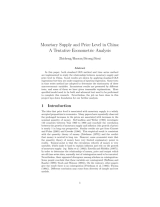
Figure 1 shows full sample of observation between Year 1978 and
2012, which provides an intuitive illustration of the dynamic evolution
of CPI/M0/M2/GDP from 1978. From the figure, we can see that: 1)
All these Macroeconomic data are growing versus time; 2) GDP basically
grows at a constant rate. Money supply is growing faster than GDP; 3)
Before the year around 1995, the CPI grew at a relatively quick speed
3
4. 403.4288
2980.9580
22026.4658
162754.7914
1980 1990 2000 2010
Year
NormalizedIndex
GDP
M0
M2
CPI
Figure 1: China’s Monetary Supply, GDP and CPI: 1978-2012
compared with year after 1995, which coincide with the growth of Mone-
tary supply (M2 or M0). These observations seem to give us the indication
that price is growing at the growth rate of money divided by GDP. Thus
we drew Figure 2 which shows the relationship of CPI versus Money di-
vided by output at each particular time. General conclusion is that there
is high positive correlation between these two indicators. As we drew lin-
ear regression lines in this picture, we can see these points are scattered
on the two sides of regressions lines. From these stylized facts, we think
a detailed econometric study to reveal the relationship of Money supply
and Price is necessary.
4 Econometrics analysis
4.1 Basic Model
Base on equation 3 in the Theory part and the annual data we got, we
build regression model like below:
pt = α + β · (mt − yt) + µt (4)
where the index t represents the annual data at particular year (t=Year-
1978). In such case, we treat the velocity of money as a value which has
constant mean α and disturbance µt at each time t. Consequently, our
approach is doing a regression according to equation 4 and testing whether
the coefficient β is close to one or whether it is significant. However, this
specified functional form of quantity equation may not be fully satisfied
even in long run empirically. Then we consider another weak form of
QTM as below:
pt = α + β1 · mt + β2 · yt + µt (5)
4
6. 148.4132
403.4288
1.000000 7.389056
Money divided by output
CPI
M0/GDP
M2/GDP
Figure 2: CPI Versus Money Divided by Output in Sample
In this weak form, we loose the constraint that mt and −yt have same
coefficient, but we still expect that β1 > 0 and β2 < 0. In other words,
intuitively, this weak form states that, with Y held constant, P would
increase as M increases; with M held constant, P tends to decrease when
Y is increasing.
Therefore, under some specific assumptions which would be mentioned
below, we can begin to do regressions base on equation 4 and 5., and
then initiate corresponding econometrics analysis. As some readers may
discover, here we are using a static model to treat these time series data,
which may lose theory foundation. However, this would not impede us
to do this first step analysis, and later we can testify that whether these
analyses are applicable.
4.2 Assumptions
1. Annual Data of these Macroeconomic variables (GDP, Consumption,
M0, M2, and CPI) are already in or close to long run equilibrium
status. This means we can deal with these variables(in Annual Data)
base on QTM.
2. The circulation velocity of money follows normal distribution which
has a mean of constant value. This indicates that the disturbance
item µt also follows a normal distribution, which has mean value of
zero.
3. The disturbance item µt is uncorrelated with explanatory variables,
i.e., E(µt|Xt) = 0, where Xt = [mt, yt]. This meanwhile authorizes
some test statics we will use below.
6
7. 4. As we firstly utilize static analysis to deal with the time series data,
here we need impose a very strong assumption that variable itself
don’t have auto-time correlation. This authorizes us that in the first
step we don’t need use time series method.
Although these assumptions are very strong and some of them may not
be realistic, we can do our econometric analysis tentatively at the very
beginning. Then as following tests to verify these assumptions are carried
out, more substantial issues would be revealed, which will also enlighten
us to develop further analysis to handle this problem.
4.3 Results
As we have mentioned above, we do static regression according to equa-
tion 4 and 5. First following equation 4, we regress CPI just on single
variable M0/GDP and M2/GDP respectively. The results are shown in
Table 2. It can be seen that all the coefficients are positive and significant,
and the F-statistic are large. Also the Goodness of Fitness (R2
) are very
high in both case, i.e., regression fit the data very well. Merely from this
table, we can tell the coefficient of M0/GDP is more close to 1 compare
with M2/GDP.
Table 2: Regression results 1
Dependent variable:
log(CPI)
(1) (2)
log(M0/GDP) 0.804∗∗∗
(0.032)
log(M2/GDP) 0.569∗∗∗
(0.015)
Constant 4.422∗∗∗
5.089∗∗∗
(0.053) (0.022)
Observations 35 35
R2
0.951 0.977
Adjusted R2
0.950 0.976
Residual Std. Error (df = 33) 0.139 0.096
F Statistic (df = 1; 33) 641.676∗∗∗
1,385.442∗∗∗
Note: ∗
p<0.1; ∗∗
p<0.05; ∗∗∗
p<0.01
Next we use the weak form (equation 5) to regress CPI on two ex-
planatory variables. As GDP includes all the output of Consumption,
Investment and Net export, CPI only reflect the price of consumption
7
8. goods, it is logical to try Consumption as an alternative of output. Thus,
here we have 4 kinds of regression methods:
1) log(CPI) ∼ log(M0) + log(GDP);
2) log(CPI) ∼ log(M2) + log(GDP);
3) log(CPI) ∼ log(M0) + log(Consumption);
4) log(CPI) ∼ log(M2) + log(Consumption).
The results of these 4 regressions are reported in Table 3. Similar with
single variable regression, all the coefficients are significant in 4 equations.
Moreover, as we expected, the coefficients of Money supply (either M0 or
M2) are positive, and the coefficients of Output (either GDP or Con-
sumption) are negative. All the F Statistics and R2
are good, suggesting
that these regressions perform well. Nevertheless, the credibility depends
on all the assumptions made previously. Therefore, next we are going to
develop methods to test those assumptions.
Table 3: Regression results 2
Dependent variable:
log(CPI)
(1) (2) (3) (4)
log(M0) 0.508∗∗∗
0.546∗∗∗
(0.065) (0.079)
log(M2) 0.915∗∗∗
1.032∗∗∗
(0.072) (0.109)
log(GDP) −0.262∗∗
−1.301∗∗∗
(0.114) (0.150)
log(Cons) −0.363∗∗
−1.712∗∗∗
(0.151) (0.254)
Constant 3.840∗∗∗
8.539∗∗∗
4.312∗∗∗
10.401∗∗∗
(0.566) (0.707) (0.739) (1.181)
Observations 35 35 35 35
R2
0.972 0.987 0.972 0.982
Adjusted R2
0.970 0.986 0.971 0.980
Residual Error (df = 32) 0.107 0.074 0.106 0.086
F Statistic (df = 2; 32) 554.778∗∗∗
1,183.905∗∗∗
561.416∗∗∗
854.661∗∗∗
Note: ∗
p<0.1; ∗∗
p<0.05; ∗∗∗
p<0.01
8
9. 4.4 Test of Assumptions
4.4.1 Disturbance
The assumptions regarding to the disturbance item µt are that:
1. µt is uncorrelated with explanatory variables, i.e., E(µt|Xt) = 0;
2. µt follows normal distribution which has mean zero.
The first one entitles the coefficient obtained by OLS is a consistent es-
timator. The second assumption authorize the validity of F-test and the
indication of F-Statistics and t-Statistics.
4.5 5.0 5.5 6.0
−0.20.00.10.2
lm(log(CPI))~log(M0)+log(GDP)
Fitted values
Residuals
Residuals vs Fitted
19
1 20
−2 −1 0 1 2
−1012
lm(log(CPI))~log(M0)+log(GDP)
Theoretical Quantiles
Standardizedresiduals
Normal Q−Q
119
20
4.5 5.0 5.5 6.0
−0.100.000.10
lm(log(CPI))~log(M2)+log(GDP)
Fitted values
Residuals
Residuals vs Fitted
1 1819
−2 −1 0 1 2
−1012
lm(log(CPI))~log(M2)+log(GDP)
Theoretical Quantiles
Standardizedresiduals
Normal Q−Q
1
1819
Figure 3: Diagnostics of Error Items in Two Regression Model
In order to verify these assumptions, we utilize diagnosis of regression,
which is shown in Figure 3. Here we only pick two regressions for il-
lustration. Two plots above diagnose CPI versus M0 and GDP, while
the below two apply to regression of CPI on M2 and GDP. The left
one tells how residuals distribute versus fitted value: The more residuals
distributed stochastically around zero, the more disturbance behave like
E(µt|Xt) = 0. The right one compares residual distribution with normal
distribution: If two quantiles locate on or near the dash line (iso-quantiles
line), it means that residuals act like normal distributions. Observation
of these plots suggests that disturbance item in regressing CPI on M2 and
9
10. GDP is likely to satisfy these two assumptions while regression of MO
and GDP is not. One possible conjecture is that compared with M2, M0
is a factor that generated endogenously in market activities. Thus, the
disturbance item at certain time t would correlate with the variable M0.
4.4.2 Spurious Regression
Another striking finding in these regression results is that the value of R2
is very high. Merely from the perspective of static regression, it imply
that the fitness of these models to the data is very good. However, can
we say that they are good regressions? Or do these regressions predicting
power? The answer is pending because here we may encounter a problem
of spurious regression.
What is spurious regression? A very simple example for illustration is
that, if we regress the GDP of China on the forest coverage of America, a
positive correlation can be obtained even they apparently have no relation.
Thus, conceptually, when two different unrelated non-stationary series are
regressed on each other, the result is usually a so-called spurious regres-
sion, in which the OLS estimates and t-statistics indicate that a relation
exists when, while in reality there is no relation. Granger and Newbold
(1974) gave a empirical feature of a potential spurious regressions is that
R2
> DW. Consequently, a DW test is implemented and the result is
shown in Table 4, suggesting that we may have spurious regressions.
Table 4: DW Test Results
Regression Model:
log(CPI) ∼ log(M0) + log(GDP) log(CPI) ∼ log(M2) + log(GDP)
DW 0.3089 0.6803
R2
0.9702 0.9858
P-value 1.268 × e−13
3.437 × e−7
Note: Alternative hypothesis: true autocorrelation is greater than 0
Another observation from the DW test is that both regressions we
choose reject the null hypothesis, i.e., accept alternative hypothesis that
true autocorrelation is greater that 0. In order to verify this verdict, we
develop a lag regression model. For these two specified situations, the
regression equations are:
1) log(CPI) ∼ log(M2) + log(GDP) + L(log(CPI)
2) log(CPI) ∼ log(M0) + log(GDP) + L(log(CPI)
The principle is to regress dependent variable on the explanatory variables
together with the dependent variable of one period ahead. Table 5 presents
the results that the coefficient of the lagged CPI is prominently significant
and the model fits data very well as R2
basically equals one, i.e, on the
other hand prove the DW test result.
Back to the discussion of spurious regression, here we briefly introduce
the theory. Engle and Granger (1987) did a test based on OLS estimation
10
11. Table 5: Regression on Lag item
Dependent variable:
log(CPI)
(1) (2)
log(M0) −1.234 × 10⁻¹⁶∗∗∗
(1.04 × 10⁻⁶
)
log(M2) −4.733 × 10⁻¹⁶∗∗∗
(2.53 × 10⁻⁹
)
log(GDP) 5.909 × 10−17∗
6.812 × 10−16∗∗∗
(0.013312) (1.26 × 10⁻⁸
)
L(log(CPI)) 1.000∗∗∗
1.000∗∗∗
(2 × 10⁻¹⁶
) (2 × 10⁻¹⁶
)
Constant −7.225 × 10⁻¹⁶∗∗∗
−3.992 × 10⁻¹⁵∗∗∗
(0.000102) (2.53 × 10⁻⁸
)
Observations 35 35
Adjusted R2
1.000 1.000
Residual Std. Error (df = 31) 1.957 × 10⁻¹⁷
2.383 × 10⁻¹⁷
F Statistic (df = 3; 31) 1.13 × 1034∗∗∗
7.62 × 1033∗∗∗
Note: ∗
p<0.1; ∗∗
p<0.05; ∗∗∗
p<0.01
of the regression
y1t = µ + γ y2t + z∗
t (6)
where y1tis the first element of yt, y2t is the vector of the remaining
n − 1 elements, and z∗
t is an error term. This regression would be a
cointegrating regression if h = 1 and y1t were part of the cointegrating
relationship. Under the null of h = 0 (no cointegration), however, this
regression does not represent a cointergrating relationship. Let (µ, γ)
be the OLS coefficient estimates of (µ, γ). it turns out that γ does not
provide consistent estimates of any population parameters of the system.
For example, even if y1t is unrelated to y2t (in that y1t and y2s) are
independent for all s , t ), the t− and F − statistics associated with the
OLS estimates become arbitrarily large as the sample size increases, giving
a false impression that there is a close connection between y1t and y2t .
This phenomenon, called the “spurious regression”, was first discovered
in Monte Carlo experiments by Granger and Newbold (1974). Phillips
(1986) theoretically derived the large-sample distribution of the statistics
for spurious regressions. For example, the t-value, if divided by
√
T ,
11
12. converges to a nondegenerate distribution.
4.4.3 Stationarity and KPSS Test
In general, regression models for non-stationary variables give spurious re-
sults. Only one exception happens when the model eliminates the stochas-
tic trends, and produces stationary residuals: Cointegration. In mathe-
matics, strictly stationary process is a stochastic process whose joint prob-
ability distribution does not change when shifted in time. But this is not
easy to verify. So in practice, we only test weak stationarity, which only
requires 1st moment and covariance. Below is the requirement of weak
stationarity:
E(Yt) = µ; V ar(Yt) = σ2
; Cov(Yt, Yt+k) = γk (7)
As we have observed from Figure 1, all variables are increasing versus
time. According to equation 7, they are obviously non-stationary. How-
ever, if variables are trend stationary, i.e., stochastically fluctuate around
a certain upward trend, they could also be used for regression or predic-
tion by detrend. Consequently, here we need test whether these variables
are trend stationary. One tentative method that may achieve this func-
tion is using KPSS test included in package ‘tseries’. Kwiatkowski et al.
(1992) proposed this test, whose null hypothesis is that an observable
is stationary around a deterministic trend. In KPSS test, the series yt
is expressed as the sum of a deterministic trend, a random walk, and a
stationary error, as in below equation:
yt = ξ · t + rt + εt (8)
Here rt is a random walk:
rt = rt−1 + ut (9)
where ut is iid (0, σ2
u). The test is the LM test whose hypothesis is that
the random walk has zero variance. The asymptotic distribution of the
statistic is derived under the null and under the alternative that the series
is difference-stationary.
Table 6: KPSS Test Results
Variables in Time Series:
CPI M0 M2 GDP
KPSS Trend 0.3628 0.4502 0.4039 0.0571
Truncation lag parameter 1 1 1 1
P-value 0.01∗∗∗
0.01∗∗∗
0.01∗∗∗
0.1
Note: Null hypothesis: Series is trend stationary
∗∗∗
p-value smaller than printed p-value
Table 6 give the results of KPSS test. We can see that CPI, M0, and
M2 reject the null hypothesis that data is trend stationary while GDP does
12
13. not. But can we justify that GDP is a trend stationary variable? The
answer is not certain. Because KPSS test may not demonstrate enough
power to reject the null. Two reasons are possible. First, the statistic is
based on asymptotic theory, while our sample size may not big enough
to exhibit this property. Second, back to Figure 1, the GDP growth
rate is relatively constant comparing with other variables, which may
cause other series are more easily to reject the null. Similar result is got
from Kwiatkowski et al. (1992) by applying KPSS test to Nelson-Plosser
data, that many macroeconomic series cannot reject the null even they
are non-stationary from other evidence. Therefore, in order to identify
the stationary property, we need employ other methods.
4.4.4 Unit Root Test
Another important test to judge whether one time series is stationary is
standard Unit Root test. In this paper, we choose two kinds of Unit Root
test Augmented Dickey-Fuller(ADF) test (Dickey and Fuller (1981)) and
Phillips-Perron(PP) test (Phillips and Perron (1988)) to implement the
research. The most significant difference between KPSS test and Unit
Root test is that the null hypothesis assuming the time series variables
have a unit root, i.e. its a I(1) process and not stationary. In Augmented
Dickey-Fuller test, the procedure is the same as for the Dickey-Fuller test
but it is applied to the model
yt = α + βt + γyt−1 + δ1 yt−1 + · · · + δp−1 yt−p−1 + εt (10)
Where α is a constant, β the coefficient on a time trend, p the lag order
of the autoregressive process and the first difference operator. What is
the main different between DF test and ADF test? It is that ADF test
addresses the issue that the process generating data for yt might have a
higher order of autocorrelation. So ADF test introduces lags of yt as
regressors in the test equation. Imposing the constraints α = 0 and β = 0
corresponds to modeling a random walk and using the constraint β = 0
corresponds to modeling a random walk with a drift. Consequently, there
are three main versions of the test. The unit root test is then carried
out under the null hypothesis γ = 0 against the alternative hypothesis of
γ < 0. Once a value for the test statistic
DFτ =
γ
SE(γ)
(11)
is computed it can be compared to the relevant critical value for the
DickeyFuller Test. If the test statistic is less (this test is non-symmetrical
so we do not consider an absolute value) than the (larger negative) critical
value, then the null hypothesis that γ = 0 is rejected and no unit root is
present. In Phillips-Perron test, we regress yt on the model
yt = α + ρyt−1 + εt (12)
which is very similar to ADF test. It also addresses the issue of higher
order autocorrelation. But instead of introducing lags of yt, PP test
makes a non-parametric correction to the t-test statistic. The test is
13
14. Table 7: ADF and PP Test
ADF Test:
CPI M0 M2 GDP
Dickey-Fuller -1.2794 -0.7893 -0.7129 -4.6319
Lag order 3 3 3 3
P-value 0.8528 0.953 0.9595 0.01∗∗∗
Note: Alternative hypothesis: Stationary
∗∗∗
p-value smaller than printed p-value
PP Test:
CPI M0 M2 GDP
Dickey-Fuller -0.9222 -0.7262 -0.4059 -2.8114
Truncation lag parameter 3 3 3 3
P-value 0.9354 0.9584 0.9803 0.258
Note: Alternative hypothesis: Stationary
robust with respect to unspecified autocorrelation and heteroscedasticity
in the disturbance process εt of the test equation.
Table 7 gives the results of ADF test and PP test. We can see that
CPI, M0, M2 have same result in both test, i.e., they all have a very large
P-value and accept the null that data have unit root. But for GDP, it
rejected the null in ADF test and accept the null in PP test simultane-
ously. Why is that? There are some possible reasons: 1. PP test is based
on asymptotic theory. It means that the test is effective under large sam-
ples. Unfortunately, we only got annual data for 35 years. Furthermore,
Davidson and MacKinnon (2004) report that the PhillipsPerron test per-
forms worse in finite samples than the Augmented DickeyFuller test. So
the result of PP test may be not so reliable. 2. The unit root is the null
hypothesis to be tested, and the way in which classical hypothesis test
is carried out ensures that the null hypothesis is accepted unless there is
strong evidence against it. So the common failure to reject a unit root test
is simply that most economic time series are not very informative to judge
whether there is a unit root, i.e., that test is not very powerful against
relevant alternatives. In Table 7, we can see that the P value of GDP in
PP test is relatively small, but not small enough to reject the null. Thus,
it could be inferred that PP test may not exhibit enough information to
reject the null.
So combined the previous result of KPSS test, we tend to believe that
the GDP data we are using here is more like a trend stationary variable.
Another aspect that may support this verdict is that in recent 30 years,
China’s GDP keeps growing in a relative constant rate: 7% to 10%. We
can define this growth rate as a constant value g and GDP is yt. Thus:
yt = (1 + g) · yt−1 ⇐⇒ yt = (1 + g)t
· y0 (13)
14
15. Take logarithm on both sides, we have:
log(yt) = t · log(1 + g) + log(y0) (14)
which on the other hand endorse that log(GDP) in recent China is likely
to be trend stationary.
In order to do cointegraton test in the future, we need know which
order of difference is stationary for each variable. Here we present results
of ADF test (Table 8) and PP test (Table 9) on the first order and second
order difference of all variables. Discrepancies exist among these two tests,
while we cannot determine which one is more credible for each variable.
Further analysis need to be done to accomplish this task.
Table 8: Result of ADF Test
PP Test:
Dickey-Fuller Lag orders p-value
∆(CPI) -2.6464 3 0.3225
∆(M0) -2.8077 3 0.26
∆(M2) -2.668 3 0.3142
∆(GDP) -3.6988 3 0.04021
∆2
(CPI) -4.5266 3 0.01∗∗∗
∆2
(M0) -4.0486 3 0.01983∗
∆2
(M2) -2.6441 3 0.3239
∆2
(GDP) -3.1447 3 0.1304
Note: Alternative hypothesis: Stationary
∗∗∗
p-value smaller than printed p-value
Table 9: Result of PP Test
PP Test:
Dickey-Fuller Truncation lag parameter p-value
∆(CPI) -2.7847 3 0.269
∆(M0) -4.762 3 0.01∗∗∗
∆(M2) -3.1584 3 0.1242
∆(GDP) -2.9068 3 0.2216
∆2
(CPI) -4.8578 3 0.01∗∗∗
∆2
(M0) -9.5772 3 0.01∗∗∗
∆2
(M2) -7.2421 3 0.01∗∗∗
∆2
(GDP) -4.7217 3 0.01∗∗∗
Note: Alternative hypothesis: Stationary
∗∗∗
p-value smaller than printed p-value
15
16. 5 Flaws in Project
Model
1. Annual data of these macroeconomic variables are not certainly in a
long-run equilibrium status. Thus, they may not satisfy the quantity
equation theoretically.
2. Velocity of money is not necessarily a constant. It may be impacted
by many factors, such as the monetary income, expenditure struc-
ture of residents, industrial structures, or development of financial
market.
Data
1. Although the degree of marketization is increasing after 1978, China
is not a country with a complete market economy. Prices of some
commodities are still controlled or regulated by the government.
This means price index may not perfectly reflect the market.
2. Variables in our data are inconsistent in statistical definition :
CPI just represent consumption price, which doesn’t include the
price of housing market, and other fixed asset or investment.
GDP consists all the outputs of consumption, investment, and net
export.
M0 is the summation of currency in circulation, which doesn’t pos-
sess property of exogenousness. While M2 is more like a exogenous
variable including all the currency in stock.
Method
1. All variables are non-stationary, so standard regressions are not valid
unless variables are cointegrated.
2. Some tests we used are based on asymptotic theory. While in this
project we only have 35 data in one series, which is not a large
sample.
6 Conclusion and Future plan
6.1 Conclusion
In this project, based on quantity theory of money, a standard OLS
method is applied to study the relationship between monetary supply
and price level in China firstly. No matter we use M0 or M2 as monetary
supply, or use GDP or consumption as output, we all get very good statis-
tics result in these regressions. However, the extraordinary high value of
R2
reminds us that we may encounter spurious regression. Subsequent
DW test and regressing on lag item confirm our speculation we make, i.e.,
these variables are autocorrelated and we may have spurious regression.
Then KPSS test is performed to determine whether the data we use are
stationary. The results show CPI,M0, and M2 are non-stationary, but
16
17. GDP are trend stationary. Combined it with the results of other two
types of Unit root tests, which are ADF test and PP test, we are inclined
to believe CPI, M0 and M2 are non-stationary with unit root process, but
GDP data in recent China is trend stationary without unit root. However,
when the two types of Unit Root tests (ADF and PP test) are executed to
the differences of each variables, inconsistent results are got. The reason
is not very clear so far and which test is more credible is to be determined
. Thus, more analysis and following cointegration test need to be done in
our future work.
6.2 Future Plan: Next Semester
1. Determine which level of difference of each variable is stationary.
Then do cointegration test on the variables which have the same
order of unit root process. If variables in one regression equation
are cointegrated, we believe that they satisfy this equation and the
regression is not spurious.
2. Even we get variables are cointegrated, i.e, they satisfy long-run
equilibrium. We can further look at the deviation relationship in the
short run, which we can do by using Error correction model (ECM:
A dynamical system with the characteristics that the deviation of
the current state from its long-run relationship will be fed into its
short-run dynamics).
3. We may add more variables into the original model, e.g, variables
that impact the circulation velocity of money. Or we can replace CPI
with some other price index that could represent output comprehen-
sively. Then we can look for more information that how variables
influence the price level in China.
References
Baba, Y., D. F. Hendry, and R. M. Starr (1992). The demand for m1 in
the usa, 1960–1988. The Review of Economic Studies 59(1), 25–61.
Blejer, M. I. and A. Cheasty (1991). The measurement of fiscal deficits:
analytical and methodological issues. Journal of Economic Literature,
1644–1678.
Chow, G. C. (1987). Money and price level determination in china. Journal
of Comparative Economics 11(3), 319–333.
Davidson, R. and J. G. MacKinnon (2004). Econometric theory and meth-
ods, Volume 21. Oxford University Press New York.
Dickey, D. A. and W. A. Fuller (1981). Likelihood ratio statistics for
autoregressive time series with a unit root. Econometrica: Journal of
the Econometric Society, 1057–1072.
Engle, R. F. and C. W. Granger (1987). Co-integration and error correc-
tion: representation, estimation, and testing. Econometrica: journal of
the Econometric Society, 251–276.
17
18. Estrella, A. and F. S. Mishkin (1997). Is there a role for monetary ag-
gregates in the conduct of monetary policy? Journal of monetary
economics 40(2), 279–304.
Friedman, B. M. and K. N. Kuttner (1992). Money, income, prices, and
interest rates. The American Economic Review, 472–492.
Friedman, B. M., K. N. Kuttner, B. S. Bernanke, and M. Gertler (1993).
Economic activity and the short-term credit markets: An analysis of
prices and quantities. brookings Papers on economic Activity, 193–283.
Friedman, M. (1956). Studies in the Quantity Theory of Money (First
ed.). Chicago, IL:: University of Chicago Press.
Friedman, M. (1970). A Theoretical Framework for Monetary Analysis.
Journal of Political Economy 78(2), 193–238.
Friedman, M. (1989). Quantity theory of money. J. Eatwell et al, 1–40.
Geweke, J. F. (1986). The superneutrality of money in the united states:
An interpretation of the evidence. Econometrica 54(1), 1–21.
Granger, C. W. and P. Newbold (1974). Spurious regressions in econo-
metrics. Journal of econometrics 2(2), 111–120.
Grauwe, P. and M. Polan (2005). Is Inflation Always and Everywhere a
Monetary Phenomenon? Scandinavian Journal of Economics 107(2),
239–59.
Hasan, M. S. (1999). Monetary Growth and Inflation in China: A Reex-
amination. Journal of Comparative Economics 27, 669–685.
Hayashi, F. (2000). Econometrics. Princeton: Princeton University Press.
Hoffman, D. and R. H. Rasche (1989). Long-run income and interest
elasticities of money demand in the united states. Technical report,
National Bureau of Economic Research.
Kwiatkowski, D., P. C. Phillips, P. Schmidt, and Y. Shin (1992). Testing
the null hypothesis of stationarity against the alternative of a unit root:
How sure are we that economic time series have a unit root? Journal
of econometrics 54(1), 159–178.
Li, K. W. and W. S. Leung (1994). Causal relationships among economic
aggregates in china. Applied economics 26(12), 1189–1196.
McCandless, T. G. and W. E. Weber (1995). Some Monetary Facts.
Federal Reserve Bank of Minneapolis Quarterly Review 19, 2–11.
Peebles, G. (1992). Why the quantity theory of money is not applicable
to china, together with a tested theory that is. Cambridge Journal of
Economics 16(1), 23–42.
Phillips, P. C. (1986). Understanding spurious regressions in econometrics.
Journal of econometrics 33(3), 311–340.
18
19. Phillips, P. C. and P. Perron (1988). Testing for a unit root in time series
regression. Biometrika 75(2), 335–346.
Stock, J. H. and M. W. Watson (1993). A simple estimator of cointegrating
vectors in higher order integrated systems. Econometrica: Journal of
the Econometric Society, 783–820.
Thoma, M. A. (1994). Subsample instability and asymmetries in money-
income causality. Journal of Econometrics 64(1), 279–306.
Zhao, L. and Y. Wang (2005). Money stock and price level in china: A
empirical evidence. Economic Sciences 2, 26–38.
19