SlideShare a Scribd company logo
1 of 59
Download to read offline
Elementary Introduction to Quantum Fields in
Curved Spacetime
Lecture notes by Sergei Winitzki
Heidelberg, April 18-21, 2006
Contents
Preface . . . . . . . . . . . . . . . . . . . . . . . . . . . . . . . . . . . . . . . 2
Suggested literature . . . . . . . . . . . . . . . . . . . . . . . . . . . . . . . . 3
1 Quantization of harmonic oscillator 3
1.1 Canonical quantization . . . . . . . . . . . . . . . . . . . . . . . . . . . 3
1.2 Creation and annihilation operators . . . . . . . . . . . . . . . . . . . 4
1.3 Particle number eigenstates . . . . . . . . . . . . . . . . . . . . . . . . 5
2 Quantization of scalar field 6
2.1 Classical field . . . . . . . . . . . . . . . . . . . . . . . . . . . . . . . . 6
2.2 Quantization of scalar field . . . . . . . . . . . . . . . . . . . . . . . . 7
2.3 Mode expansions . . . . . . . . . . . . . . . . . . . . . . . . . . . . . . 9
3 Casimir effect 9
3.1 Zero-point energy . . . . . . . . . . . . . . . . . . . . . . . . . . . . . . 9
3.2 Casimir effect . . . . . . . . . . . . . . . . . . . . . . . . . . . . . . . . 10
3.3 Zero-point energy between plates . . . . . . . . . . . . . . . . . . . . . 10
3.4 Regularization and renormalization . . . . . . . . . . . . . . . . . . . 13
4 Oscillator with varying frequency 14
4.1 Quantization . . . . . . . . . . . . . . . . . . . . . . . . . . . . . . . . . 14
4.2 Choice of mode function . . . . . . . . . . . . . . . . . . . . . . . . . . 16
4.3 “In” and “out” states . . . . . . . . . . . . . . . . . . . . . . . . . . . . 17
4.4 Relationship between “in” and “out” states . . . . . . . . . . . . . . . 19
4.5 Quantum-mechanical analogy . . . . . . . . . . . . . . . . . . . . . . 20
5 Scalar field in expanding universe 21
5.1 Curved spacetime . . . . . . . . . . . . . . . . . . . . . . . . . . . . . 21
5.2 Scalar field in cosmological background . . . . . . . . . . . . . . . . . 22
5.3 Mode expansion . . . . . . . . . . . . . . . . . . . . . . . . . . . . . . . 23
5.4 Quantization of scalar field . . . . . . . . . . . . . . . . . . . . . . . . 24
5.5 Vacuum state and particle states . . . . . . . . . . . . . . . . . . . . . 25
5.6 Bogolyubov transformations . . . . . . . . . . . . . . . . . . . . . . . 25
5.7 Mean particle number . . . . . . . . . . . . . . . . . . . . . . . . . . . 26
5.8 Instantaneous lowest-energy vacuum . . . . . . . . . . . . . . . . . . 27
5.9 Computation of Bogolyubov coefficients . . . . . . . . . . . . . . . . . 27
1
6 Amplitude of quantum fluctuations 29
6.1 Fluctuations of averaged fields . . . . . . . . . . . . . . . . . . . . . . 29
6.2 Fluctuations in Minkowski spacetime . . . . . . . . . . . . . . . . . . 30
6.3 de Sitter spacetime . . . . . . . . . . . . . . . . . . . . . . . . . . . . . 30
6.4 Quantum fields in de Sitter spacetime . . . . . . . . . . . . . . . . . . 31
6.5 Bunch-Davies vacuum state . . . . . . . . . . . . . . . . . . . . . . . . 32
6.6 Spectrum of fluctuations in the BD vacuum . . . . . . . . . . . . . . . 33
7 Unruh effect 33
7.1 Kinematics of uniformly accelerated motion . . . . . . . . . . . . . . 34
7.2 Coordinates in the proper frame . . . . . . . . . . . . . . . . . . . . . 35
7.3 Rindler spacetime . . . . . . . . . . . . . . . . . . . . . . . . . . . . . . 38
7.4 Quantum field in Rindler spacetime . . . . . . . . . . . . . . . . . . . 38
7.5 Lightcone mode expansions . . . . . . . . . . . . . . . . . . . . . . . . 41
7.6 Bogolyubov transformations . . . . . . . . . . . . . . . . . . . . . . . . 42
7.7 Density of particles . . . . . . . . . . . . . . . . . . . . . . . . . . . . . 44
7.8 Unruh temperature . . . . . . . . . . . . . . . . . . . . . . . . . . . . . 47
8 Hawking radiation 47
8.1 Scalar field in Schwarzschild spacetime . . . . . . . . . . . . . . . . . 48
8.2 Kruskal coordinates . . . . . . . . . . . . . . . . . . . . . . . . . . . . . 49
8.3 Field quantization . . . . . . . . . . . . . . . . . . . . . . . . . . . . . . 50
8.4 Choice of vacuum . . . . . . . . . . . . . . . . . . . . . . . . . . . . . . 51
8.5 Hawking temperature . . . . . . . . . . . . . . . . . . . . . . . . . . . 52
8.6 Black hole thermodynamics . . . . . . . . . . . . . . . . . . . . . . . . 53
A Hilbert spaces and Dirac notation 55
A.1 Infinite-dimensional vector spaces . . . . . . . . . . . . . . . . . . . . 55
A.2 Dirac notation . . . . . . . . . . . . . . . . . . . . . . . . . . . . . . . . 55
A.3 Hermiticity . . . . . . . . . . . . . . . . . . . . . . . . . . . . . . . . . 56
A.4 Hilbert spaces . . . . . . . . . . . . . . . . . . . . . . . . . . . . . . . . 57
B Mode expansions cheat sheet 58
Preface
This course is a brief introduction to Quantum Field Theory in Curved Spacetime
(QFTCS)—a beautiful and fascinating area of fundamental physics. The applica-
tion of QFTCS is required in situations when both gravitation and quantum me-
chanics play a significant role, for instance, in early-universe cosmology and black
hole physics. The goal of this course is to introduce some of the most accessible
aspects of quantum theory in nontrivial backgrounds and to explain its most unex-
pected and spectacular manifestations—the Casimir effect (uncharged metal plates
attract), the Unruh effect (an accelerated observer will detect particles in vacuum),
and Hawking’s theoretical discovery of black hole radiation (black holes are not
completely black).
This short course was taught in the framework of Heidelberger Graduiertenkurse
at the Heidelberg University (Germany) in the Spring of 2006. The audience in-
cluded advanced undergraduates and beginning graduate students. Only a basic
familiarity with quantum mechanics, electrodynamics, and general relativity is re-
quired. The emphasis is on concepts and intuitive explanations rather than on
computational techniques. The relevant calculations are deliberately simplified
as much as possible, while retaining all the relevant physics. Some remarks and
derivations are typeset in smaller print and can be skipped at first reading.
2
These lecture notes are freely based on an early draft of the book [MW07] with
some changes appropriate for the purposes of the Heidelberg course. The present
text may be freely distributed according to the GNU Free Documentation License.1
Sergei Winitzki, April 2006
Suggested literature
The following more advanced books may be studied as a continuation of this in-
troductory course:
[BD82] N. D. BIRRELL and P. C. W. DAVIES, Quantum fields in curved space
(Cambridge University Press, 1982).
[F89] S. A. FULLING, Aspects of quantum field theory in curved space-time (Cam-
bridge University Press, 1989).
[GMM94] A. A. GRIB, S. G. MAMAEV, and V. M. MOSTEPANENKO, Vacuum
quantum effects in strong fields (Friedmann Laboratory Publishing, St. Petersburg,
1994).
The following book contains a significantly more detailed presentation of the
material of this course, and much more:
[MW07] V. F. MUKHANOV and S. WINITZKI, Quantum Effects in Gravity (to be
published by Cambridge University Press, 2007).2
1 Quantization of harmonic oscillator
This section serves as a very quick reminder of quantum mechanics of harmonic
oscillators. It is assumed that the reader is already familiar with such notions as
Schrödinger equation and Heisenberg picture.
1.1 Canonical quantization
A classical harmonic oscillator is described by a coordinate q(t) satisfying
¨q + ω2
q = 0, (1)
where ω is a real constant. The general solution of this equation can be written as
q(t) = aeiωt
+ a∗
e−iωt
,
where a is a (complex-valued) constant. We may identify the “ground state” of the
oscillator as the state without motion, i.e. q(t) ≡ 0. This is obviously the lowest-
energy state of the oscillator.
The quantum theory of the oscillator is obtained by the standard procedure
known as canonical quantization. Canonical quantization does not apply directly
to an equation of motion. Rather, we first need to describe the system using the
Hamiltonian formalism, which means that we must start with the Lagrangian ac-
tion principle. The classical equation of motion (1) is reformulated as a condition
to extremize the action,
L(q, ˙q)dt =
1
2
˙q2
−
1
2
ω2
q2
dt,
1See www.gnu.org/copyleft/fdl.html
2An early, incomplete draft is available at www.theorie.physik.uni-muenchen.de/~serge/T6/
3
where the function L(q, ˙q) is the Lagrangian. (For simplicity, we assumed a unit
mass of the oscillator.) Then we define the canonical momentum
p ≡
∂L(q, ˙q)
∂ ˙q
= ˙q,
and perform a Legendre transformation to find the Hamiltonian
H(p, q) ≡ [p ˙q − L]˙q→p =
1
2
p2
+
1
2
ω2
q2
.
The Hamiltonian equations of motion are
˙q = p, ˙p = −ω2
q.
Finally, we replace the classical coordinate q(t) and the momentum p(t) by Hermi-
tian operators ˆq(t) and ˆp(t) satisfying the same equations of motion,
˙ˆq = ˆp, ˙ˆp = −ω2
ˆq,
and additionally postulate the Heisenberg commutation relation
[ˆq(t), ˆp(t)] = i . (2)
The Hamiltonian H(p, q) is also promoted to an operator,
ˆH ≡ H(ˆp, ˆq) =
1
2
ˆp2
+
1
2
ω2
ˆq2
.
All the quantum operators pertaining to the oscillator act in a certain vector space
of quantum states or wavefunctions. (This space must be a Hilbert space; see Ap-
pendix A for details.) Vectors from this space are usually denoted using Dirac’s
“bra-ket” symbols: vectors are denoted by |a , |b , and the corresponding covec-
tors by a|, b|, etc. Presently, we use the Heisenberg picture, in which the opera-
tors depend on time but the quantum states are time-independent. This picture is
more convenient for developing quantum field theory than the Schrödinger pic-
ture where operators are time-independent but wavefunctions change with time.
Therefore, we shall continue to treat the harmonic oscillator in the Heisenberg pic-
ture. We shall not need to use the coordinate or momentum representation of
wavefunctions.
1.2 Creation and annihilation operators
The “classical ground state” ˆq(t) ≡ 0 is impossible in quantum theory because in
that case the commutation relation (2) could not be satisfied by any ˆp(t). Hence, a
quantum oscillator cannot be completely at rest, and its lowest-energy state (called
the ground state or the vacuum state) has a more complicated structure. The stan-
dard way of describing quantum oscillators is through the introduction of the cre-
ation and annihilation operators.
From now on, we use the units where = 1. The Heisenberg commutation
relation becomes
[ˆq(t), ˆp(t)] = i. (3)
We now define the annihilation operator ˆa−
(t) and its Hermitian conjugate, cre-
ation operator ˆa+
(t), by
ˆa±
(t) =
ω
2
ˆq(t) ∓
i
ω
ˆp(t) .
4
These operators are not Hermitian since (ˆa−
)†
= ˆa+
. The equation of motion for
the operator ˆa−
(t) is straightforward to derive,
d
dt
ˆa−
(t) = −iωˆa−
(t). (4)
(The Hermitian conjugate operator ˆa+
(t) satisfies the complex conjugate equation.)
The solution of Eq. (4) with the initial condition ˆa−
(t)|t=0 = ˆa−
0 can be readily
found,
ˆa−
(t) = ˆa−
0 e−iωt
. (5)
It is helpful to introduce time-independent operators ˆa±
0 ≡ ˆa±
and to write the
time-dependent phase factor eiωt
explicitly. For instance, we find that the canonical
variables ˆp(t), ˆq(t) are related to ˆa±
by
ˆp(t) =
√
ω
ˆa−
e−iωt
− ˆa+
eiωt
i
√
2
, ˆq(t) =
ˆa−
e−iωt
+ ˆa+
eiωt
√
2ω
. (6)
From now on, we shall only use the time-independent operators ˆa±
. Using Eqs. (3)
and (6), it is easy to show that
[ˆa−
, ˆa+
] = 1.
Using the relations (6), the operator ˆH can be expressed through the creation and
annihilation operators ˆa±
as
ˆH = ˆa+
ˆa−
+
1
2
ω. (7)
1.3 Particle number eigenstates
Quantum states of the oscillator are described by vectors in an appropriate (infinite-
dimensional) Hilbert space. A complete basis in this space is made of vectors |0 ,
|1 , ..., which are called the occupation number states or particle number states.
The construction of these states is well known, and we briefly review it here for
completeness.
It is seen from Eq. (7) that the eigenvalues of ˆH are bounded from below by
1
2 ω. It is then assumed that the ground state |0 exists and is unique. Using this
assumption and the commutation relations, one can show that the state |0 satisfies
ˆa−
|0 = 0.
(This derivation is standard and we omit it here.) Then we have ˆH |0 = 1
2 ω |0 ,
which means that the ground state |0 indeed has the lowest possible energy 1
2 ω.
The excited states |n , where n = 1, 2, ..., are defined by
|n =
1
√
n!
(ˆa+
)n
|0 . (8)
The factors
√
n! are needed for normalization, namely m|n = δmn. It is easy to
see that every state |n is an eigenstate of the Hamiltonian,
ˆH |n = n +
1
2
ω |n .
In other words, the energy of the oscillator is quantized (not continuous) and is mea-
sured in discrete “quanta” equal to ω. Therefore, we might interpret the state |n
as describing the presence of n “quanta” of energy or n “particles,” each “particle”
5
having the energy ω. (In normal units, the energy of each quantum is ω, which
is the famous Planck formula for the energy quantum.) The operator ˆN ≡ ˆa+
ˆa−
is called the particle number operator. Since ˆN |n = n |n , the states |n are also
called particle number eigenstates. This terminology is motivated by the applica-
tions in quantum field theory (as we shall see below).
To get a feeling of what the ground state |0 looks like, one can compute the ex-
pectation values of the coordinate and the momentum in the state |0 . For instance,
using Eq. (6) we find
0| ˆq(t) |0 = 0, 0| ˆp(t) |0 = 0,
0| ˆq2
(t) |0 =
1
2ω
, 0| ˆp2
(t) |0 =
ω
2
.
It follows that the ground state |0 of the oscillator exhibits fluctuations of both the
coordinate and the momentum around a zero mean value. The typical value of the
fluctuation in the coordinate is δq ∼ (2ω)
−1/2
.
2 Quantization of scalar field
The quantum theory of fields is built on two essential foundations: the classical
theory of fields and the quantum mechanics of harmonic oscillators.
2.1 Classical field
A classical field is described by a function of spacetime, φ (x, t), characterizing the
local strength or intensity of the field. Here x is a three-dimensional coordinate in
space and t is the time (in some reference frame). The function φ (x, t) may have
real values, complex values, or values in some finite-dimensional vector space. For
example, the electromagnetic field is described by the 4-potential Aµ(x, t), which
is a function whose values are 4-vectors.
The simplest example of a field is a real scalar field φ (x, t); its values are real
numbers. A free, massive scalar field satisfies the Klein-Gordon equation3
∂2
φ
∂t2
−
3
j=1
∂2
φ
∂x2
j
+ m2
φ ≡ ¨φ − ∆φ + m2
φ ≡ ∂µ∂µ
φ + m2
φ = 0. (9)
The parameter m is the mass of the field. The solution φ (x, t) ≡ 0 is the classical
vacuum state (“no field”).
To simplify the equations of motion, it is convenient to use the spatial Fourier
decomposition,
φ (x, t) =
d3
k
(2π)3/2
eik·x
φk(t), (10)
where we integrate over all three-dimensional vectors k. After the Fourier decom-
position, the partial differential equation (9) is replaced by infinitely many ordi-
nary differential equations, with one equation for each k:
¨φk + k2
+ m2
φk = ¨φk + ω2
kφk = 0, ωk ≡ |k|
2
+ m2.
In other words, each function φk(t) satisfies the harmonic oscillator equation with
the frequency ωk. The complex-valued functions φk(t) are called the modes of the
3To simplify the formulas, we shall (almost always) use the units in which = c = 1.
6
field φ (abbreviated from “Fourier modes”). Note that the modes φk(t) of a real
field φ(x, t) satisfy the relation (φk)∗
= φ−k.
The equation of motion (9) can be found by extremizing the action
S [φ] =
1
2
d4
x ηµν
(∂µφ) (∂νφ) − m2
φ2
≡
1
2
d3
x dt ˙φ2
− (∇φ)2
− m2
φ2
, (11)
where ηµν
= diag(1, −1, −1, −1) is the Minkowski metric (in this chapter we con-
sider only the flat spacetime) and the Greek indices label four-dimensional coor-
dinates: x0
≡ t and (x1
, x2
, x3
) ≡ x. Using Eq. (10), one can also express the
action (11) directly through the (complex-valued) modes φk,
S =
1
2
dt d3
k ˙φk
˙φ∗
k − ω2
kφkφ∗
k . (12)
2.2 Quantization of scalar field
The action (12) is analogous to that of a collection of infinitely many harmonic
oscillators. Therefore, we may quantize each mode φk(t) as a separate (complex-
valued) harmonic oscillator.
Let us begin with the Hamiltonian description of the field φ(x, t). The ac-
tion (11) must be thought of as an integral of the Lagrangian over time (but not
over space), S[φ] = L[φ] dt, so the Lagrangian L[φ] is
L[φ] = Ld3
x; L ≡
1
2
ηµν
(∂µφ) (∂νφ) −
1
2
m2
φ2
,
where L is the Lagrangian density. To define the canonical momenta and the
Hamiltonian, one must use the Lagrangian L[φ] rather than the Lagrangian density
L. Hence, the momenta π (x, t) are computed as the functional derivatives
π (x, t) ≡
δL [φ]
δ ˙φ (x, t)
= ˙φ (x, t) ,
and then the classical Hamiltonian is
H = π (x, t) ˙φ (x, t) d3
x − L =
1
2
d3
x π2
+ (∇φ)2
+ m2
φ2
. (13)
To quantize the field, we introduce the operators ˆφ (x, t) and ˆπ (x, t) with the
standard commutation relations
[ˆφ (x, t) , ˆπ (y, t)] = iδ (x − y) ; [ˆφ (x, t) , ˆφ (y, t)] = [ˆπ (x, t) , ˆπ (y, t)] = 0. (14)
The modes φk(t) also become operators ˆφk(t). The commutation relation for the
modes can be derived from Eq. (14) by performing Fourier transforms in x and y.
After some algebra, we find
ˆφk(t), ˆπk′ (t) = iδ (k + k′
) . (15)
Note the plus sign in δ(k1 + k2): this is related to the fact that the variable which is
conjugate to ˆφk is not ˆπk but ˆπ−k = ˆπ†
k.
7
Remark: complex oscillators. The modes φk(t) are complex variables; each φk may be
thought of as a pair of real-valued oscillators, φk = φ
(1)
k + iφ
(2)
k . Accordingly, the oper-
ators ˆφk are not Hermitian and (ˆφk)†
= ˆφ−k. In principle, one could rewrite the theory
in terms of Hermitian variables such as φ
(1,2)
k and π
(1,2)
k with standard commutation
relations, h
φ
(1)
k , π
(1)
k′
i
= iδ(k − k′
),
h
φ
(2)
k , π
(2)
k′
i
= iδ(k − k′
)
but it is technically more convenient to keep the complex-valued modes φk. The non-
standard form of the commutation relation (15) is a small price to pay.
For each mode φk, we proceed with the quantization as in Sec. 1.2. We first
introduce the time-dependent creation and annihilation operators:
ˆa−
k (t) ≡
ωk
2
ˆφk +
iˆπk
ωk
; ˆa+
k (t) ≡
ωk
2
ˆφ−k −
iˆπ−k
ωk
.
Note that (ˆa−
k )†
= ˆa+
k . The equations of motion for the operators ˆa±
k (t),
d
dt
ˆa±
k (t) = ±iωkˆa±
k (t),
have the general solution ˆa±
k (t) = (0)
ˆa±
k e±iωkt
, where the time-independent opera-
tors (0)
ˆa±
k satisfy the relations (note the signs of k and k′
)
ˆa−
k , ˆa+
k′ = δ (k − k′
) ; ˆa−
k , ˆa−
k′ = ˆa+
k , ˆa+
k′ = 0. (16)
In Eq. (16) we omitted the superscript (0)
for brevity; below we shall always use
the time-independent creation and annihilation operators and denote them by ˆa±
k .
The Hilbert space of field states is built in the standard fashion. We postulate
the existence of the vacuum state |0 such that ˆa−
k |0 = 0 for all k. The state with
particle numbers ns in each mode with momentum ks (where s = 1, 2, ... is an
index that enumerates the excited modes) is defined by
|n1, n2, ... =
s
ˆa+
ks
ns
√
ns!
|0 . (17)
We write |0 instead of |0, 0, ... for brevity. The Hilbert space of quantum states
is spanned by the vectors |n1, n2, ... with all possible choices of the numbers ns.
This space is called the Fock space.
The quantum Hamiltonian of the free scalar field can be written as
ˆH =
1
2
d3
k ˆπkˆπ−k + ω2
k
ˆφk
ˆφ−k ,
and expressed through the creation and annihilation operators as
ˆH = d3
k
ωk
2
ˆa−
k ˆa+
k + ˆa+
k ˆa−
k = d3
k
ωk
2
2ˆa+
k ˆa−
k + δ(3)
(0) . (18)
Derivation of Eq. (18)
We use the relations
ˆφk =
1
√
2ωk
“
ˆa−
k e−iωkt
+ ˆa+
−keiωkt
”
, ˆπk = i
r
ωk
2
“
ˆa+
−keiωkt
− ˆa−
k e−iωkt
”
.
(Here ˆa±
k are time-independent operators.) Then we find
1
2
“
ˆπk ˆπ−k + ω2
k
ˆφk
ˆφ−k
”
=
ωk
2
`
ˆa−
k ˆa+
k + ˆa+
−kˆa−
−k
´
.
8
When we integrate over all k, the terms with −k give the same result as the terms with
k. Therefore ˆH = 1
2
R
d3
k
`
ˆa+
k ˆa−
k + ˆa−
k ˆa+
k
´
ωk.
Thus we have quantized the scalar field φ(x, t) in the Heisenberg picture. Quan-
tum observables such as ˆφ(x, t) and ˆH are now represented by linear operators in
the Fock space, and the quantum states of the field φ are interpreted in terms of
particles. Namely, the state vector (17) is interpreted as a state with ns particles
having momentum ks (where s = 1, 2, ...). This particle interpretation is consistent
with the relativistic expression for the energy of a particle, E = p2 + m2, if we
identify the 3-momentum p with the wavenumber k and the energy E with ωk.
2.3 Mode expansions
We now give a brief introduction to mode expansions, which offer a shorter and
computationally convenient way to quantize fields. A more detailed treatment is
given in Sec 5.
The quantum mode ˆφk(t) can be expressed through the creation and annihila-
tion operators,
ˆφk(t) =
1
√
2ωk
ˆa−
k e−iωkt
+ ˆa+
−keiωkt
.
Substituting this into Eq. (10), we obtain the following expansion of the field oper-
ator ˆφ (x, t),
ˆφ (x, t) =
d3
k
(2π)3/2
1
√
2ωk
ˆa−
k e−iωkt+ik·x
+ ˆa+
−keiωkt+ik·x
,
which we then rewrite by changing k → −k in the second term to make the inte-
grand manifestly Hermitian:
ˆφ (x, t) =
d3
k
(2π)3/2
1
√
2ωk
ˆa−
k e−iωkt+ik·x
+ ˆa+
k eiωkt−ik·x
. (19)
This expression is called the mode expansion of the quantum field ˆφ.
It is easy to see that the Klein-Gordon equation (9) is identically satisfied by
the ansatz (19) with arbitrary time-independent operators ˆa±
k . In fact, Eq. (19) is a
general solution of Eq. (9) with operator-valued “integration constants” ˆa±
k . On the
other hand, one can verify that the commutation relations (15) between ˆφk and ˆπk
are equivalent to Eq. (16). Therefore, we may view the mode expansion (19) as a
convenient shortcut to quantizing the field φ (x, t). One simply needs to postulate
the commutation relations (16) and the mode expansion (19), and then the opera-
tors ˆφk and ˆπk do not need to be introduced explicitly. The Fock space of quantum
states is constructed directly through the operators ˆa±
k and interpreted as above.
3 Casimir effect
3.1 Zero-point energy
The zero-point energy is the energy of the vacuum state. We saw in Sec. 2.2 that a
quantum field is equivalent to a collection of infinitely many harmonic oscillators.
If the field φ is in the vacuum state, each oscillator φk is in the ground state and
has the energy 1
2 ωk. Hence, the total zero-point energy of the field is the sum of
1
2 ωk over all wavenumbers k. This sum may be approximated by an integral in the
9
following way: If one quantizes the field in a box of large but finite volume V , one
will obtain the result that the zero-point energy density is equal to
E0
V
=
d3
k
(2π)
3
1
2
ωk.
(A detailed computation can be found in the book [MW07].) Since ωk grows with
k, it is clear that the integral diverges. Taken at face value, this would indicate
an infinite energy density of the vacuum state. Since any energy density leads
to gravitational effects, the presence of a nonzero energy density in the vacuum
state contradicts the experimental observation that empty space does not generate
any gravitational force. The standard way to avoid this problem is to subtract
this infinite quantity from the energy of the system (“renormalization” of zero-
point energy). In other words, the ground state energy 1
2 ωk is subtracted from
the Hamiltonian of each oscillator φk. A justification for this subtraction is that
the ground state energy cannot be extracted from an oscillator, and that only the
change in the oscillator’s energy can be observed.
3.2 Casimir effect
The Casimir effect is an experimentally verified prediction of quantum field theory.
It is manifested by a force of attraction between two uncharged conducting plates in
a vacuum. This force cannot be explained except by considering the zero-point en-
ergy of the quantized electromagnetic field. The presence of the conducting plates
makes the electromagnetic field vanish on the surfaces of the plates. This boundary
condition changes the structure of vacuum fluctuations of the field, which would
normally be nonzero on the plates. This change causes a finite shift ∆E of the
zero-point energy, compared with the zero-point energy in empty space without
the plates. The energy shift ∆E = ∆E(L) depends on the distance L between the
plates, and it turns out that ∆E grows with L. As a result, it is energetically fa-
vorable for the plates to move closer together, which is manifested as the Casimir
force of attraction between the plates,
F(L) = −
d
dL
[∆E(L)] .
This theoretically predicted force has been confirmed by several experiments.4
3.3 Zero-point energy between plates
A realistic description of the Casimir effect involves quantization of the electro-
magnetic field in the presence of conductors having certain dielectric properties;
thermal fluctuations must also be taken into account. We shall drastically sim-
plify the calculations by considering a massless scalar field φ(t, x) in the flat 1+1-
dimensional spacetime. To simulate the presence of the plates, we impose the fol-
lowing boundary conditions:
φ(t, x)|x=0 = φ(t, x)|x=L = 0. (20)
The equation of motion for the classical field is ∂2
t φ − ∂2
xφ = 0, and the general
solution for the chosen boundary conditions is of the form
φ(t, x) =
∞
n=1
Ane−iωnt
+ Bneiωnt
sin ωnx, ωn ≡
nπ
L
.
4For example, a recent measurement of the Casimir force to 1% precision is described in: U. MO-
HIDEEN and A. ROY, Phys. Rev. Lett. 81 (1998), p. 4549.
10
We shall now use this solution as a motivation for finding the appropriate mode
expansion for the field φ.
To quantize the field φ(t, x) in flat space, one would normally use the mode
expansion
ˆφ(t, x) =
dk
(2π)1/2
1
√
2ωk
ˆa−
k e−iωkt+ikx
+ ˆa+
k eiωkt−ikx
.
However, in the present case the only allowed modes are those satisfying Eq. (20),
so the above mode expansion cannot be used. To expand the field ˆφ(t, x) into the
allowed modes, we use the orthogonal system of functions
gn(x) =
2
L
sin
nπx
L
which vanish at x = 0 and x = L. These functions satisfy the orthogonality relation
L
0
gm(x)gn(x)dx = δmn.
(The coefficient 2/L is necessary for the correct normalization.) An arbitrary
function F(x) that vanishes at x = 0 and x = L can be expanded through the
functions gn(x) as
F(x) =
∞
n=1
Fngn(x),
where the coefficients Fn are found as
Fn =
L
0
F(x)gn(x)dx.
Performing this decomposition for the field operator ˆφ(t, x), we find
ˆφ(t, x) =
∞
n=1
ˆφn(t)gn(x),
where ˆφn(t) is the n-th mode of the field. The mode ˆφn(t) satisfies the oscillator
equation
¨ˆφn +
πn
L
2
ˆφn ≡
¨ˆφn + ω2
n
ˆφn = 0, (21)
whose general solution is
ˆφn(t) = ˆAe−iωnt
+ ˆBeiωnt
,
where ˆA, ˆB are operator-valued integration constants. After computing the correct
normalization of these constants (see below), we obtain the the mode expansion for
ˆφ as
ˆφ(t, x) =
2
L
∞
n=1
sin ωnx
√
2ωn
ˆa−
n e−iωnt
+ ˆa+
n eiωnt
. (22)
We need to compute the energy of the field only between the plates, 0 < x < L.
After some calculations (see below), one can express the zero-point energy per unit
length as
ε0 ≡
1
L
0| ˆH |0 =
1
2L
k
ωk =
π
2L2
∞
n=1
n. (23)
11
Derivation of Eqs. (22) and (23)
We use the following elementary identities which hold for integer m, n:
Z L
0
dx sin
mπx
L
sin
nπx
L
=
Z L
0
dx cos
mπx
L
cos
nπx
L
=
L
2
δmn. (24)
First, let us show that the normalization factor
p
2/L in the mode expansion (22)
yields the standard commutation relations
ˆ
ˆa−
m, ˆa+
n
˜
= δmn. We integrate the mode
expansion over x and use the identity (24) to get
Z L
0
dx ˆφ(x, t) sin ωnx =
1
2
r
L
ωn
h
ˆa−
n e−iωnt
+ ˆa+
n eiωnt
i
.
Then we differentiate this with respect to t and obtain
Z L
0
dx′
ˆπ(y, t) sin ωnx′
=
i
2
√
Lωn
h
−ˆa−
n e−iωnt
+ ˆa+
n eiωnt
i
.
Now we can evaluate the commutator
»Z L
0
dx ˆφ(x, t) sin ωnx,
Z L
0
dy
d
dt
ˆφ(x′
, t) sin ωn′ x′
–
= i
L
2
ˆ
ˆa−
n , ˆa+
n′
˜
=
Z L
0
dx
Z L
0
dx′
sin
nπx
L
sin
n′
πx′
L
iδ(x − x′
) = i
L
2
δnn′ .
In the second line we used
h
ˆφ(x, t), ˆπ(x′
, t)
i
= iδ(x − x′
). Therefore the standard
commutation relations hold for ˆa±
n .
The Hamiltonian for the field (restricted to the region between the plates) is
ˆH =
1
2
Z L
0
dx
"
∂ ˆφ(x, t)
∂t
!2
+
∂ ˆφ(x, t)
∂x
!2#
.
The expression 0| ˆH |0 is evaluated using the mode expansion above and the relations
0| ˆa−
mˆa+
n |0 = δmn, 0| ˆa+
mˆa+
n |0 = 0| ˆa−
mˆa−
n |0 = 0| ˆa+
mˆa−
n |0 = 0.
The first term in the Hamiltonian yields
0|
1
2
Z L
0
dx
∂ ˆφ(x, t)
∂t
!2
|0
= 0|
1
2
Z L
0
dx
"r
2
L
∞X
n=1
sin ωnx
√
2ωn
iωn
“
−ˆa−
n e−iωnt
+ ˆa+
n eiωnt
”
#2
|0
=
1
L
Z L
0
dx
∞X
n=1
(sin ωnx)2
2ωn
ω2
n =
1
4
X
n
ωn.
The second term gives the same result, and we find
0| ˆH |0 =
1
2
∞X
n=1
ωn.
Therefore, the energy density (the energy per unit length) is given by Eq. (23).
12
3.4 Regularization and renormalization
The zero-point energy density ε0 is divergent. However, in the presence of the
plates the energy density diverges in a different way than in free space because
ε0 = ε0(L) depends on the distance L between the plates. The zero-point energy
density in free space can be thought of as the limit of ε0(L) at L → ∞,
ε
(free)
0 = lim
L→∞
ε0 (L) .
When the zero-point energy is renormalized in free space, the infinite contribu-
tion ε
(free)
0 is subtracted. Thus we are motivated to subtract ε
(free)
0 from the energy
density ε0(L) and to expect to find a finite difference ∆ε between these formally
infinite quantities,
∆ε (L) = ε0 (L) − ε
(free)
0 = ε0 (L) − lim
L→∞
ε0 (L) . (25)
In the remainder of the chapter we calculate this energy difference ∆ε(L).
Taken at face value, Eq. (25) is meaningless because the difference between two
infinite quantities is undefined. The standard way to deduce reasonable answers
from infinities is a regularization followed by a renormalization. A regularization
means introducing an extra parameter into the theory to make the divergent quan-
tity finite unless that parameter is set to (say) zero. Such regularization parame-
ters or cutoffs can be chosen in many ways. After the regularization, one derives
an asymptotic form of the divergent quantity at small values of the cutoff. This
asymptotic may contain divergent powers and logarithms of the cutoff as well as
finite terms. Renormalization means removing the divergent terms and leaving
only the finite terms in the expression. (Of course, a suitable justification must be
provided for subtracting the divergent terms.) After renormalization, the cutoff is
set to zero and the remaining terms yield the final result. If the cutoff function is
chosen incorrectly, the renormalization procedure will not succeed. It is usually
possible to motivate the correct choice of the cutoff by physical considerations.
We shall now apply this procedure to Eq. (25). As a first step, a cutoff must be
introduced into the divergent expression (23). One possibility is to replace ε0 by
the regularized quantity
ε0 (L; α) =
π
2L2
∞
n=1
n exp −
nα
L
, (26)
where α is the cutoff parameter. The regularized series converges for α > 0, while
the original divergent expression is recovered in the limit α → 0.
Remark: choosing the cutoff function. We regularize the series by the factor exp(−nα/L)
and not by exp(−nα) or exp(−nLα). A motivation is that the physically significant
quantity is ωn = πn/L, therefore the cutoff factor should be a function of ωn. Also,
renormalization will fail if the regularization is chosen incorrectly.
Now we need to evaluate the regularized quantity (26) and to analyze its asymp-
totic behavior at α → 0. A straightforward computation gives
ε0 (L; α) = −
π
2L
∂
∂α
∞
n=1
exp −
nα
L
=
π
2L2
exp −α
L
1 − exp −α
L
2 .
At α → 0 this expression can be expanded in a Laurent series,
ε0 (L; α) =
π
8L2
1
sinh2 α
2L
=
π
2α2
−
π
24L2
+ O α2
. (27)
13
The series (27) contains the singular term π
2 α−2
, a finite term, and further terms
that vanish as α → 0. The crucial fact is that the singular term in Eq. (27) does not
depend on L. (This would not have happened if we chose the cutoff e.g. as e−nα
.)
The limit L → ∞ in Eq. (25) is taken before the limit α → 0, so the divergent term
π
2 α−2
cancels and the renormalized value of ∆ε is finite,
∆εren(L) = lim
α→0
ε0 (L; α) − lim
L→∞
ε0 (L; α) = −
π
24L2
. (28)
The formula (28) is the main result of this chapter; the zero-point energy density
is nonzero in the presence of plates at x = 0 and x = L. The Casimir force between
the plates is
F = −
d
dL
∆E = −
d
dL
(L∆εren) = −
π
24L2
.
Since the force is negative, the plates are pulled toward each other.
Remark: negative energy. Note that the zero-point energy density (28) is negative.
Quantum field theory generally admits quantum states with a negative expectation
value of energy.
4 Oscillator with varying frequency
A gravitational background influences quantum fields in such a way that the fre-
quencies ωk of the modes become time-dependent, ωk(t). We shall examine this
situation in detail in chapter 5. For now, let us consider a single harmonic oscilla-
tor with a time-dependent frequency ω(t).
4.1 Quantization
In the classical theory, the coordinate q(t) satisfies
¨q + ω2
(t)q = 0. (29)
An important example of a function ω(t) is shown Fig. 1. The frequency is approx-
imately constant except for a finite time interval, for instance ω ≡ ω0 for t ≤ t0 and
ω ≡ ω1 for t ≥ t1. It is usually impossible to find an exact solution of Eq. (29) in
such cases (of course, an approximate solution can be found numerically). How-
ever, the solutions in the regimes t ≤ t0 and t ≥ t1 are easy to obtain:
q(t) = Aeiω0t
+ Be−iω0t
, t ≤ t0;
q(t) = Aeiω1t
+ Be−iω1t
, t ≥ t1.
We shall be interested only in describing the behavior of the oscillator in these two
regimes5
which we call the “in” and “out” regimes.
The classical equation of motion (29) can be derived from the Lagrangian
L (t, q, ˙q) =
1
2
˙q2
−
1
2
ω(t)2
q2
.
The corresponding canonical momentum is p = ˙q, and the Hamiltonian is
H(p, q) =
p2
2
+ ω2
(t)
q2
2
, (30)
5In the physics literature, the word regime stands for “an interval of values for a variable.” It should
be clear from the context which interval for which variable is implied.
14
ω(t)
ω1
ω0
t0 t1
t
Figure 1: A frequency function ω(t) with “in” and “out” regimes (at t ≤ t0 and
t ≥ t1).
which depends explicitly on the time t. Therefore, we do not expect that energy
is conserved in this system. (There is an external agent that drives ω(t) and may
exchange energy with the oscillator.)
A time-dependent oscillator can be quantized using the technique of creation
and annihilation operators. By analogy with Eq. (6), we try the ansatz
ˆq(t) =
1
√
2
v(t)ˆa+
+ v∗
(t)ˆa−
, ˆp(t) =
1
√
2
˙v(t)ˆa+
+ ˙v∗
(t)ˆa−
, (31)
where v(t) is a complex-valued function that replaces eiωt
, while the operators
ˆa±
are time-independent. The present task is to choose the function v(t) and the
operators ˆa±
in an appropriate way. We call v(t) the mode function because we
shall later apply the same decomposition to modes of a quantum field.
Since ˆq(t) must be a solution of Eq. (29), we find that v(t) must satisfy the same
equation,
¨v + ω2
(t)v = 0. (32)
Furthermore, the canonical commutation relation [ˆq(t), ˆp(t)] = i entails
ˆa−
, ˆa+
=
2i
˙vv∗ − ˙v∗v
.
Note that the expression
˙vv∗
− ˙v∗
v ≡ W[v, v∗
]
is the Wronskian of the solutions v(t) and v∗
(t), and it is well known that W =
const. We may therefore normalize the mode function v(t) such that
W[v, v∗
] = ˙vv∗
− ˙v∗
v = 2i, (33)
which will yield the standard commutation relations for ˆa±
,
ˆa−
, ˆa+
= 1.
We can then postulate the existence of the ground state |0 such that ˆa−
|0 = 0.
Excited states |n (n = 1, 2, ...) are defined in the standard way by Eq. (8).
With the normalization (33), the creation and annihilation operators are ex-
pressed through the canonical variables as
ˆa−
≡
˙v(t)ˆq(t) − v(t)ˆp(t)
i
√
2
, ˆa+
≡ −
˙v∗
(t)ˆq(t) − v∗
(t)ˆp(t)
i
√
2
. (34)
(Note that the l.h.s. of Eq. (34) are time-independent because the corresponding
r.h.s. are Wronskians.) In this way, a choice of the mode function v(t) defines the
operators ˆa±
and the states |0 , |1 , ...
15
It is clear that different choices of v(t) will in general define different operators
ˆa±
and different states |0 , |1 , ... It is not clear, a priori, which choice of v(t) cor-
responds to the “correct” ground state of the oscillator. The choice of v(t) will be
studied in the next section.
Properties of mode functions
Here is a summary of some elementary properties of a time-dependent oscillator
equation
¨x + ω2
(t)x = 0. (35)
This equation has a two-dimensional space of solutions. Any two linearly independent
solutions x1(t) and x2(t) are a basis in that space. The expression
W [x1, x2] ≡ ˙x1x2 − x1 ˙x2
is called the Wronskian of the two functions x1(t) and x2(t). It is easy to see that
the Wronskian W [x1, x2] is time-independent if x1,2(t) satisfy Eq. (35). Moreover,
W [x1, x2] = 0 if and only if x1(t) and x2(t) are two linearly independent solutions.
If {x1(t), x2(t)} is a basis of solutions, it is convenient to define the complex func-
tion v(t) ≡ x1(t) + ix2(t). Then v(t) and v∗
(t) are linearly independent and form a
basis in the space of complex solutions of Eq. (35). It is easy to check that
Im(˙vv∗
) =
˙vv∗
− ˙v∗
v
2i
=
1
2i
W [v, v∗
] = −W [x1, x2] = 0,
and thus the quantity Im(˙vv∗
) is a nonzero real constant. If v(t) is multiplied by a
constant, v(t) → λv(t), the Wronskian W [v, v∗
] changes by the factor |λ|2
. Therefore
we may normalize v(t) to a prescribed value of Im(˙vv∗
) by choosing the constant λ, as
long as v and v∗
are linearly independent solutions so that W [v, v∗
] = 0.
A complex solution v(t) of Eq. (35) is an admissible mode function if v(t) is nor-
malized by the condition Im(˙vv∗
) = 1. It follows that any solution v(t) normalized by
Im(˙vv∗
) = 1 is necessarily complex-valued and such that v(t) and v∗
(t) are a basis of
linearly independent complex solutions of Eq. (35).
4.2 Choice of mode function
We have seen that different choices of the mode function v(t) lead to different defi-
nitions of the operators ˆa±
and thus to different “canditate ground states” |0 . The
true ground state of the oscillator is the lowest-energy state and not merely some
state |0 satisfying ˆa−
|0 = 0, where ˆa−
is some arbitrary operator. Therefore we
may try to choose v(t) such that the mean energy 0| ˆH |0 is minimized.
For any choice of the mode function v(t), the Hamiltonian is expressed through
the operators ˆa±
as
ˆH =
|˙v|
2
+ ω2
|v|
2
4
2ˆa+
ˆa−
+ 1 +
˙v2
+ ω2
v2
4
ˆa+
ˆa+
+
˙v∗2
+ ω2
v∗2
4
ˆa−
ˆa−
. (36)
Derivation of Eq. (36)
In the canonical variables, the Hamiltonian is
ˆH =
1
2
ˆp2
+
1
2
ω2
(t)ˆq2
.
Now we expand the operators ˆp, ˆq through the mode functions using Eq. (31) and the
commutation relation
ˆ
ˆa+
, ˆa−
˜
= 1. For example, the term ˆp2
gives
ˆp2
=
1
√
2
`
˙v(t)ˆa+
+ ˙v∗
(t)ˆa−´ 1
√
2
`
˙v(t)ˆa+
+ ˙v∗
(t)ˆa−´
=
1
2
`
˙v2
ˆa+
ˆa+
+ ˙v ˙v∗ `
2ˆa+
ˆa−
+ 1
´
+ ˙v∗2
ˆa−
ˆa−´
.
16
The term ˆq2
gives
ˆq2
=
1
√
2
`
v(t)ˆa+
+ v∗
(t)ˆa−
´ 1
√
2
`
v(t)ˆa+
+ v∗
(t)ˆa−
´
=
1
2
`
v2
ˆa+
ˆa+
+ vv∗
`
2ˆa+
ˆa−
+ 1
´
+ v∗2
ˆa−
ˆa−
´
.
After some straightforward algebra we obtain the required result.
It is easy to see from Eq. (36) that the mean energy at time t is given by
E(t) ≡ 0| ˆH(t) |0 =
| ˙v(t)|
2
+ ω2
(t) |v(t)|
2
4
. (37)
We would like to find the mode function v(t) that minimizes the above quantity.
Note that E(t) is time-dependent, so we may first try to minimize E(t0) at a fixed
time t0.
The choice of the mode function v(t) may be specified by a set of initial condi-
tions at t = t0,
v(t0) = q, ˙v(t0) = p,
where the parameters p and q are complex numbers satisfying the normalization
constraint which follows from Eq. (33),
q∗
p − p∗
q = 2i. (38)
Now we need to find such p and q that minimize the expression |p|
2
+ ω2
(t0) |q|
2
.
This is a straightforward exercise (see below) which yields, for ω(t0) > 0, the fol-
lowing result:
v(t0) =
1
ω(t0)
, ˙v(t0) = i ω(t0) = iω(t0)v(t0). (39)
If, on the other hand, ω2
(t0) < 0 (i.e. ω is imaginary), there is no minimum. For
now, we shall assume that ω(t0) is real. Then the mode function satisfying Eq. (39)
will define the operators ˆa±
and the state |t0 0 such that the instantaneous energy
E(t0) has the lowest possible value Emin = 1
2 ω(t0). The state |t0 0 is called the
instantaneous ground state at time t = t0.
Derivation of Eq. (39)
If some p and q minimize |p|2
+ ω2
|q|2
, then so do eiλ
p and eiλ
q for arbitrary real λ;
this is the freedom of choosing the overall phase of the mode function. We may choose
this phase to make q real and write p = p1 + ip2 with real p1,2. Then Eq. (38) yields
q =
2i
p − p∗
=
1
p2
⇒ 4E(t0) = p2
1 + p2
2 +
ω2
(t0)
p2
2
. (40)
If ω2
(t0) > 0, the function E (p1, p2) has a minimum with respect to p1,2 at p1 = 0 and
p2 =
p
ω(t0). Therefore the desired initial conditions for the mode function are given
by Eq. (39).
On the other hand, if ω2
(t0) < 0 the function Ek in Eq. (40) has no minimum
because the expression p2
2 + ω2
(t0)p−2
2 varies from −∞ to +∞. In that case the instan-
taneous lowest-energy ground state does not exist.
4.3 “In” and “out” states
Let us now consider the frequency function ω(t) shown in Fig. 1. It is easy to see
that the lowest-energy state is given by the mode function vin(t) = eiω0t
in the
“in” regime (t ≤ t0) and by vout(t) = eiω1t
in the “out” regime (t ≥ t1). However,
17
note that vin(t) = eiω0t
for t > t0; instead, vin(t) is a solution of Eq. (29) with the
initial conditions (39) at t = t0. Similarly, vout(t) = eiω1t
for t < t1. While exact
solutions for vin(t) and vout(t) are in general not available, we may still analyze the
relationship between these solutions in the “in” and “out” regimes.
Since the solutions e±iω1t
are a basis in the space of solutions of Eq. (35), we
may write
vin(t) = αvout(t) + βv∗
out(t), (41)
where α and β are time-independent constants. The relationship (41) between the
mode functions is an example of a Bogolyubov transformation (see Sec. 2.2). Us-
ing Eq. (33) for vin(t) and vout(t), it is straightforward to derive the property
|α|
2
− |β|
2
= 1. (42)
For a general ω(t), we will have β = 0 and hence there will be no single mode
function v(t) matching both vin(t) and vout(t).
Each choice of the mode function v(t) defines the corresponding creation and
annihilation operators ˆa±
. Let us denote by ˆa±
in the operators defined using the
mode function vin(t) and vout(t), respectively. It follows from Eqs. (34) and (41)
that
ˆa−
in = αˆa−
out − βˆa+
out.
The inverse relation is easily found using Eq. (42),
ˆa−
out = α∗
ˆa−
in + βˆa+
in. (43)
Since generally β = 0, we cannot define a single set of operators ˆa±
which will
define the ground state |0 for all times.
Moreover, in the intermediate regime where ω(t) is not constant, an instanta-
neous ground state |t0 defined at time t will, in general, not be a ground state at
the next moment, t + ∆t. Therefore, such a state |t0 cannot be trusted as a phys-
ically motivated ground state. However, if we restrict our attention only to the
“in” regime, the mode function vin(t) defines a perfectly sensible ground state |0in
which remains the ground state for all t ≤ t0. Similarly, the mode function vout(t)
defines the ground state |0out .
Since we are using the Heisenberg picture, the quantum state |ψ of the oscil-
lator is time-independent. It is reasonable to plan the following experiment. We
prepare the oscillator in its ground state |ψ = |0in at some early time t < t0 within
the “in” regime. Then we let the oscillator evolve until the time t = t1 and compare
its quantum state (which remains |0in ) with the true ground state, |0out , at time
t > t1 within the “out” regime.
In the “out” regime, the state |0in is not the ground state any more, and thus it
must be a superposition of the true ground state |0out and the excited states |nout
defined using the “out” creation operator ˆa+
out,
|nout =
1
√
n!
ˆa+
out
n
|0out , n = 0, 1, 2, ...
It can be easily verified that the vectors |nout are eigenstates of the Hamiltonian
for t ≥ t1 (but not for t < t1):
ˆH(t) |nout = ω1 n +
1
2
|nout , t ≥ t1.
Similarly, the excited states |nin may be defined through the creation operator ˆa+
in.
The states |nin are interpreted as n-particle states of the oscillator for t ≤ t0, while
for t ≥ t1 the n-particle states are |nout .
18
Remark: interpretation of the “in” and “out” states. We are presently working in the
Heisenberg picture where quantum states are time-independent and operators depend
on time. One may prepare the oscillator in a state |ψ , and the state of the oscillator re-
mains the same throughout all time t. However, the physical interpretation of this state
changes with time because the state |ψ is interpreted with help of the time-dependent
operators ˆH(t), ˆa−
(t), etc. For instance, we found that at late times (t ≥ t1) the vector
|0in is not the lowest-energy state any more. This happens because the energy of the
system changes with time due to the external force that drives ω(t). Without this force,
we would have ˆa−
in = ˆa−
out and the state |0in would describe the physical vacuum at all
times.
4.4 Relationship between “in” and “out” states
The states |nout , where n = 0, 1, 2, ..., form a complete basis in the Hilbert space
of the harmonic oscillator. However, the set of states |nin is another complete
basis in the same space. Therefore the vector |0in must be expressible as a linear
combination of the “out” states,
|0in =
∞
n=0
Λn |nout , (44)
where Λn are suitable coefficients. If the mode functions are related by a Bo-
golyubov transformation (41), one can show that these coefficients Λn are given
by
Λ2n = 1 −
β
α
2 1/4
β
α
n
(2n − 1)!!
(2n)!!
, Λ2n+1 = 0. (45)
The relation (44) shows that the early-time ground state is a superposition of
excited states at late times, having the probability |Λn|
2
for the occupation number
n. We thus conclude that the presence of an external influence leads to excitations
of the oscillator. (Later on, when we consider field theory, such excitations will be
interpreted as particle production.) In the present case, the influence of external
forces on the oscillator consists of the changing frequency ω(t), which is formally
a parameter of the Lagrangian. For this reason, the excitations arising in a time-
dependent oscillator are called parametric excitations.
Finally, let us compute the expected particle number in the “out” regime, as-
suming that the oscillator is in the state |0in . The expectation value of the number
operator ˆNout ≡ ˆa+
outˆa−
out in the state |0in is easily found using Eq. (43):
0in| ˆa+
outˆa−
out |0in = 0in| αˆa+
in + β∗
ˆa−
in α∗
ˆa−
in + βˆa+
in |0in = |β|
2
.
Therefore, a nonzero coefficient β signifies the presence of particles in the “out”
region.
Derivation of Eq. (45)
In order to find the coefficients Λn, we need to solve the equation
0 = ˆa−
in |0in =
`
αˆa−
out − βˆa+
out
´ ∞X
n=0
Λn |nout .
Using the known properties
ˆa+
|n =
√
n + 1 |n + 1 , ˆa−
|n =
√
n |n − 1 ,
we obtain the recurrence relation
Λn+2 = Λn
β
α
r
n + 1
n + 2
; Λ1 = 0.
19
Therefore, only even-numbered Λ2n are nonzero and may be expressed through Λ0 as
follows,
Λ2n = Λ0
„
β
α
«n
s
1 · 3 · ... · (2n − 1)
2 · 4 · ... · (2n)
≡ Λ0
„
β
α
«n
s
(2n − 1)!!
(2n)!!
, n ≥ 1.
For convenience, one defines (−1)!! = 1, so the above expression remains valid also for
n = 0.
The value of Λ0 is determined from the normalization condition, 0in| 0in = 1,
which can be rewritten as
|Λ0|2
∞X
n=0
˛
˛
˛
˛
β
α
˛
˛
˛
˛
2n
(2n − 1)!!
(2n)!!
= 1.
The infinite sum can be evaluated as follows. Let f(z) be an auxiliary function defined
by the series
f(z) ≡
∞X
n=0
z2n (2n − 1)!!
(2n)!!
.
At this point one can guess that this is a Taylor expansion of f(z) =
`
1 − z2
´−1/2
; then
one obtains Λ0 = 1/
p
f(z) with z ≡ |β/α|. If we would like to avoid guessing, we
could manipulate the above series in order to derive a differential equation for f(z):
f(z) = 1 +
∞X
n=1
z2n 2n − 1
2n
(2n − 3)!!
(2n − 2)!!
= 1 +
∞X
n=1
z2n (2n − 3)!!
(2n − 2)!!
−
∞X
n=1
z2n
2n
(2n − 3)!!
(2n − 2)!!
= 1 + z2
f(z) −
∞X
n=1
z2n
2n
(2n − 3)!!
(2n − 2)!!
.
Taking d/dz of both parts, we have
d
dz
ˆ
1 + z2
f(z) − f(z)
˜
=
∞X
n=1
z2n−1 (2n − 3)!!
(2n − 2)!!
= zf(z),
hence f(z) satisfies
d
dz
ˆ
(z2
− 1)f(z)
˜
=
`
z2
− 1
´ df
dz
+ 2zf(z) = zf(z); f(0) = 1.
The solution is
f(z) =
1
√
1 − z2
.
Substituting z ≡ |β/α|, we obtain the required result,
Λ0 =
"
1 −
˛
˛
˛
˛
β
α
˛
˛
˛
˛
2
#1/4
.
4.5 Quantum-mechanical analogy
The time-dependent oscillator equation (35) is formally similar to the stationary
Schrödinger equation for the wave function ψ(x) of a quantum particle in a one-
dimensional potential V (x),
d2
ψ
dx2
+ (E − V (x)) ψ = 0.
The two equations are related by the replacements t → x and ω2
(t) → E − V (x).
20
x1 x2
incoming
R
T
V (x)
x
Figure 2: Quantum-mechanical analogy: motion in a potential V (x).
To illustrate the analogy, let us consider the case when the potential V (x) is
almost constant for x < x1 and for x > x2 but varies in the intermediate region
(see Fig. 2). An incident wave ψ(x) = exp(−ipx) comes from large positive x and is
scattered off the potential. A reflected wave ψR(x) = R exp(ipx) is produced in the
region x > x2 and a transmitted wave ψT (x) = T exp(−ipx) in the region x < x1.
For most potentials, the reflection amplitude R is nonzero. The conservation of
probability gives the constraint |R|
2
+ |T |
2
= 1.
The wavefunction ψ(x) behaves similarly to the mode function v(t) in the case
when ω(t) is approximately constant at t ≤ t0 and at t ≥ t1. If the wavefunction
represents a pure incoming wave x < x1, then at x > x2 the function ψ(x) will
be a superposition of positive and negative exponents exp (±ikx). This is the phe-
nomenon known as over-barrier reflection: there is a small probability that the
particle is reflected by the potential, even though the energy is above the height of
the barrier. The relation between R and T is similar to the normalization condition
(42) for the Bogolyubov coefficients. The presence of the over-barrier reflection
(R = 0) is analogous to the presence of particles in the “out” region (β = 0).
5 Scalar field in expanding universe
Let us now turn to the situation when quantum fields are influenced by strong
gravitational fields. In this chapter, we use units where c = G = 1, where G is
Newton’s constant.
5.1 Curved spacetime
Einstein’s theory of gravitation (General Relativity) is based on the notion of
curved spacetime, i.e. a manifold with arbitrary coordinates x ≡ {xµ
} and a met-
ric gµν(x) which replaces the flat Minkowski metric ηµν. The metric defines the
interval
ds2
= gµνdxµ
dxν
,
which describes physically measured lengths and times. According to the Einstein
equation, the metric gµν(x) is determined by the distribution of matter in the entire
universe.
Here are some basic examples of spacetimes. In the absence of matter, the met-
ric is equal to the Minkowski metric ηµν = diag (1, −1, −1, −1) (in Cartesian coor-
dinates). In the presence of a single black hole of mass M, the metric can be written
in spherical coordinates as
ds2
= 1 −
2M
r
dt2
− 1 −
2M
r
−1
dr2
− r2
dθ2
+ sin2
θdφ2
.
21
Finally, a certain class of spatially homogeneous and isotropic distributions of mat-
ter in the universe yields a metric of the form
ds2
= dt2
− a2
(t) dx2
+ dy2
+ dy2
, (46)
where a(t) is a certain function called the scale factor. (The interpretation is that
a(t) “scales” the flat metric dx2
+ dy2
+ dz2
at different times.) Spacetimes with
metrics of the form (46) are called Friedmann-Robertson-Walker (FRW) spacetimes
with flat spatial sections (in short, flat FRW spacetimes). Note that it is only the
three-dimensional spatial sections which are flat; the four-dimensional geometry of
such spacetimes is usually curved. The class of flat FRW spacetimes is important in
cosmology because its geometry agrees to a good precision with the present results
of astrophysical measurements.
In this course, we shall not be concerned with the task of obtaining the metric.
It will be assumed that a metric gµν(x) is already known in some coordinates {xµ
}.
5.2 Scalar field in cosmological background
Presently, we shall study the behavior of a quantum field in a flat FRW spacetime
with the metric (46). In Einstein’s General Relativity, every kind of energy influ-
ences the geometry of spacetime. However, we shall treat the metric gµν(x) as fixed
and disregard the influence of fields on the geometry.
A minimally coupled, free, real, massive scalar field φ(x) in a curved spacetime
is described by the action
S =
√
−gd4
x
1
2
gαβ
(∂αφ) (∂βφ) −
1
2
m2
φ2
. (47)
(Note the difference between Eq. (47) and Eq. (11): the Minkowski metric ηµν is
replaced by the curved metric gµν, and the integration uses the covariant volume
element
√
−gd4
x. This is the minimal change necessary to make the theory of the
scalar field compatible with General Relativity.) The equation of motion for the
field φ is derived straightforwardly as
gµν
∂µ∂νφ +
1
√
−g
(∂νφ) ∂µ gµν√
−g + m2
φ = 0. (48)
This equation can be rewritten more concisely using the covariant derivative cor-
responding to the metric gµν,
gµν
∇µ∇νφ + m2
φ = 0,
which shows explicitly that this is a generalization of the Klein-Gordon equation
to curved spacetime.
We cannot directly use the quantization technique developed for fields in the
flat spacetime. First, let us carry out a few mathematical transformations to sim-
plify the task.
The metric (46) for a flat FRW spacetime can be simplified if we replace the
coordinate t by the conformal time η,
η(t) ≡
t
t0
dt
a(t)
,
where t0 is an arbitrary constant. The scale factor a(t) must be expressed through
the new variable η; let us denote that function again by a(η). In the coordinates
(x, η), the interval is
ds2
= a2
(η) dη2
− dx2
, (49)
22
so the metric is conformally flat (equal to the flat metric multiplied by a factor):
gµν = a2
ηµν, gµν
= a−2
ηµν
.
Further, it is convenient to introduce the auxiliary field χ ≡ a(η)φ. Then one
can show that the action (47) can be rewritten in terms of the field χ as follows,
S =
1
2
d3
x dη χ′2
− (∇χ)2
− m2
eff(η)χ2
, (50)
where the prime ′
denotes ∂/∂η, and meff is the time-dependent effective mass
m2
eff(η) ≡ m2
a2
−
a′′
a
. (51)
The action (50) is very similar to the action (11), except for the presence of the
time-dependent mass.
Derivation of Eq. (50)
We start from Eq. (47). Using the metric (49), we have
√
−g = a4
and gαβ
= a−2
ηαβ
.
Then
√
−g m2
φ2
= m2
a2
χ2
,
√
−g gαβ
φ,αφ,β = a2
`
φ′2
− (∇φ)2
´
.
Substituting φ = χ/a, we get
a2
φ′2
= χ′2
− 2χχ′ a′
a
+ χ2
„
a′
a
«2
= χ′2
+ χ2 a′′
a
−
»
χ2 a′
a
–′
.
The total time derivative term can be omitted from the action, and we obtain the re-
quired expression.
Thus, the dynamics of a scalar field φ in a flat FRW spacetime is mathematically
equivalent to the dynamics of the auxiliary field χ in the Minkowski spacetime. All
the information about the influence of gravitation on the field φ is encapsulated in
the time-dependent mass meff(η) defined by Eq. (51). Note that the action (50) is
explicitly time-dependent, so the energy of the field χ is generally not conserved.
We shall see that in quantum theory this leads to the possibility of particle creation;
the energy for new particles is supplied by the gravitational field.
5.3 Mode expansion
It follows from the action (50) that the equation of motion for χ(x, η) is
χ′′
− ∆χ + m2
a2
−
a′′
a
χ = 0. (52)
Expanding the field χ in Fourier modes,
χ (x, η) =
d3
k
(2π)3/2
χk(η)eik·x
, (53)
we obtain from Eq. (52) the decoupled equations of motion for the modes χk(η),
χ′′
k + k2
+ m2
a2
(η) −
a′′
a
χk ≡ χ′′
k + ω2
k(η)χk = 0. (54)
All the modes χk(η) with equal |k| = k are complex solutions of the same equa-
tion (54). This equation describes a harmonic oscillator with a time-dependent
frequency. Therefore, we may apply the techniques we developed in chapter 4.
23
We begin by choosing a mode function vk(η), which is a complex-valued solu-
tion of
v′′
k + ω2
k(η)vk = 0, ω2
k(η) ≡ k2
+ m2
eff(η). (55)
Then, the general solution χk(η) is expressed as a linear combination of vk and v∗
k
as
χk(η) =
1
√
2
a−
k v∗
k(η) + a+
−kvk(η) , (56)
where a±
k are complex constants of integration that depend on the vector k (but
not on η). The index −k in the second term of Eq. (56) and the factor 1√
2
are chosen
for later convenience.
Since χ is real, we have χ∗
k = χ−k. It follows from Eq. (56) that a+
k = a−
k
∗
.
Combining Eqs. (53) and (56), we find
χ (x, η) =
d3
k
(2π)3/2
1
√
2
a−
k v∗
k(η) + a+
−kvk(η) eik·x
=
d3
k
(2π)3/2
1
√
2
a−
k v∗
k(η)eik·x
+ a+
k vk(η)e−ik·x
. (57)
Note that the integration variable k was changed (k → −k) in the second term of
Eq. (57) to make the integrand a manifestly real expression. (This is done only for
convenience.)
The relation (57) is called the mode expansion of the field χ (x, η) w.r.t. the
mode functions vk(η). At this point the choice of the mode functions is still arbi-
trary.
The coefficients a±
k are easily expressed through χk(η) and vk(η):
a−
k =
√
2
v′
kχk − vkχ′
k
v′
kv∗
k − vkv∗′
k
=
√
2
W [vk, χk]
W [vk, v∗
k]
; a+
k = a−
k
∗
. (58)
Note that the numerators and denominators in Eq. (58) are time-independent since
they are Wronskians of solutions of the same oscillator equation.
5.4 Quantization of scalar field
The field χ(x) can be quantized directly through the mode expansion (57), which
can be used for quantum fields in the same way as for classical fields. The mode
expansion for the field operator ˆχ is found by replacing the constants a±
k in Eq. (57)
by time-independent operators ˆa±
k :
ˆχ (x, η) =
d3
k
(2π)3/2
1
√
2
eik·x
v∗
k(η)ˆa−
k + e−ik·x
vk(η)ˆa+
k , (59)
where vk(η) are mode functions obeying Eq. (55). The operators ˆa±
k satisfy the
usual commutation relations for creation and annihilation operators,
ˆa−
k , ˆa+
k′ = δ(k − k′
), ˆa−
k , ˆa−
k′ = ˆa+
k , ˆa+
k′ = 0. (60)
The commutation relations (60) are consistent with the canonical relations
[χ(x1, η), χ′
(x2, η)] = iδ(x1 − x2)
only if the mode functions vk(η) are normalized by the condition
Im (v′
kv∗
k) =
v′
kv∗
k − vkv′∗
k
2i
≡
W [vk, v∗
k]
2i
= 1. (61)
24
Therefore, quantization of the field ˆχ can be accomplished by postulating the mode
expansion (59), the commutation relations (60) and the normalization (61). The
choice of the mode functions vk(η) will be made later on.
The mode expansion (59) can be visualized as the general solution of the field
equation (52), where the operators ˆa±
k are integration constants. The mode expan-
sion can also be viewed as a definition of the operators ˆa±
k through the field operator
ˆχ (x, η). Explicit formulae relating ˆa±
k to ˆχ and ˆπ ≡ ˆχ′
are analogous to Eq. (58).
Clearly, the definition of ˆa±
k depends on the choice of the mode functions vk(η).
5.5 Vacuum state and particle states
Once the operators ˆa±
k are determined, the vacuum state |0 is defined as the eigen-
state of all annihilation operators ˆa−
k with eigenvalue 0, i.e. ˆa−
k |0 = 0 for all k. An
excited state |mk1 , nk2 , ... with the occupation numbers m, n, ... in the modes χk1 ,
χk2 , ..., is constructed by
|mk1 , nk2 , ... ≡
1
√
m!n!...
ˆa+
k1
m
ˆa+
k2
n
... |0 . (62)
We write |0 instead of |0k1 , 0k2 , ... for brevity. An arbitrary quantum state |ψ is a
linear combination of these states,
|ψ =
m,n,...
Cmn... |mk1 , nk2 , ... .
If the field is in the state |ψ , the probability for measuring the occupation number
m in the mode χk1 , the number n in the mode χk2 , etc., is |Cmn...|
2
.
Let us now comment on the role of the mode functions. Complex solutions
vk(η) of a second-order differential equation (55) with one normalization condi-
tion (61) are parametrized by one complex parameter. Multiplying vk(η) by a con-
stant phase eiα
introduces an extra phase e±iα
in the operators ˆa±
k , which can be
compensated by a constant phase factor eiα
in the state vectors |0 and |mk1 , nk2 , ... .
There remains one real free parameter that distinguishes physically inequivalent
mode functions. With each possible choice of the functions vk(η), the operators ˆa±
k
and consequently the vacuum state and particle states are different. As long as the
mode functions satisfy Eqs. (55) and (61), the commutation relations (60) hold and
thus the operators ˆa±
k formally resemble the creation and annihilation operators for
particle states. However, we do not yet know whether the operators ˆa±
k obtained
with some choice of vk(η) actually correspond to physical particles and whether
the quantum state |0 describes the physical vacuum. The correct commutation
relations alone do not guarantee the validity of the physical interpretation of the
operators ˆa±
k and of the state |0 . For this interpretation to be valid, the mode func-
tions must be appropriately selected; we postpone the consideration of this important
issue until Sec. 5.8 below. For now, we shall formally study the consequences of
choosing several sets of mode functions to quantize the field φ.
5.6 Bogolyubov transformations
Suppose two sets of isotropic mode functions uk(η) and vk(η) are chosen. Since uk
and u∗
k are a basis, the function vk is a linear combination of uk and u∗
k, e.g.
v∗
k(η) = αku∗
k(η) + βkuk(η), (63)
with η-independent complex coefficients αk and βk. If both sets vk(η) and uk(η)
are normalized by Eq. (61), it follows that the coefficients αk and βk satisfy
|αk|2
− |βk|2
= 1. (64)
25
In particular, |αk| ≥ 1.
Derivation of Eq. (64)
We suppress the index k for brevity. The normalization condition for u(η) is
u∗
u′
− uu′∗
= 2i.
Expressing u through v as given, we obtain
`
|α|2
− |β|2´ `
v∗
v′
− vv′∗´
= 2i.
The formula (64) follows from the normalization of v(η).
Using the mode functions uk(η) instead of vk (η), one obtains an alternative
mode expansion which defines another set ˆb±
k of creation and annihilation opera-
tors,
ˆχ (x, η) =
d3
k
(2π)3/2
1
√
2
eik·x
u∗
k(η)ˆb−
k + e−ik·x
uk(η)ˆb+
k . (65)
The expansions (59) and (65) express the same field ˆχ (x, η) through two different
sets of functions, so the k-th Fourier components of these expansions must agree,
eik·x
u∗
k(η)ˆb−
k + uk(η)ˆb+
−k = eik·x
v∗
k(η)ˆa−
k + vk(η)ˆa+
−k .
A substitution of vk through uk using Eq. (63) gives the following relation between
the operators ˆb±
k and ˆa±
k :
ˆb−
k = αkˆa−
k + β∗
k ˆa+
−k, ˆb+
k = α∗
kˆa+
k + βkˆa−
−k. (66)
The relation (66) and the complex coefficients αk, βk are called respectively the
Bogolyubov transformation and the Bogolyubov coefficients.6
The two sets of annihilation operators ˆa−
k and ˆb−
k define the corresponding
vacua (a)0 and (b)0 , which we call the “a-vacuum” and the “b-vacuum.” Two
parallel sets of excited states are built from the two vacua using Eq. (62). We refer
to these states as a-particle and b-particle states. So far the physical interpretation
of the a- and b-particles remains unspecified. Later on, we shall apply this for-
malism to study specific physical effects and the interpretation of excited states
corresponding to various mode functions will be explained. At this point, let us
only remark that the b-vacuum is in general a superposition of a-states, similarly
to what we found in Sec. 4.4.
5.7 Mean particle number
Let us calculate the mean number of b-particles of the mode χk in the a-vacuum
state. The expectation value of the b-particle number operator ˆN
(b)
k = ˆb+
k
ˆb−
k in the
state (a)0 is found using Eq. (66):
(a)0 ˆN(b)
(a)0 = (a)0 ˆb+
k
ˆb−
k (a)0
= (a)0 α∗
kˆa+
k + βkˆa−
−k αkˆa−
k + β∗
k ˆa+
−k (a)0
= (a)0 βkˆa−
−k β∗
k ˆa+
−k (a)0 = |βk|
2
δ(3)
(0). (67)
The divergent factor δ(3)
(0) is a consequence of considering an infinite spatial vol-
ume. This divergent factor would be replaced by the box volume V if we quantized
the field in a finite box. Therefore we can divide by this factor and obtain the mean
density of b-particles in the mode χk,
nk = |βk|2
. (68)
6The pronunciation is close to the American “bogo-lube-of” with the third syllable stressed.
26
The Bogolyubov coefficient βk is dimensionless and the density nk is the mean
number of particles per spatial volume d3
x and per wave number d3
k, so that
nkd3
k d3
x is the (dimensionless) total mean number of b-particles in the a-vacuum
state.
The combined mean density of particles in all modes is d3
k |βk|
2
. Note that
this integral might diverge, which would indicate that one cannot disregard the
backreaction of the produced particles on other fields and on the metric.
5.8 Instantaneous lowest-energy vacuum
In the theory developed so far, the particle interpretation depends on the choice
of the mode functions. For instance, the a-vacuum (a)0 defined above is a state
without a-particles but with b-particle density nk in each mode χk. A natural ques-
tion to ask is whether the a-particles or the b-particles are the correct representation
of the observable particles. The problem at hand is to determine the mode func-
tions that describe the “actual” physical vacuum and particles.
Previously, we defined the vacuum state as the eigenstate with the lowest en-
ergy. However, in the present case the Hamiltonian explicitly depends on time
and thus does not have time-independent eigenstates that could serve as vacuum
states.
One possible prescription for the vacuum state is to select a particular moment
of time, η = η0, and to define the vacuum |η0 0 as the lowest-energy eigenstate of
the instantaneous Hamiltonian ˆH(η0). To obtain the mode functions that describe
the vacuum |η0 0 , we first compute the expectation value (v)0 ˆH(η0) (v)0 in the
vacuum state (v)0 determined by arbitrarily chosen mode functions vk(η). Then
we can minimize that expectation value with respect to all possible choices of vk(η).
(A standard result in linear algebra is that the minimization of x| ˆA |x with respect
to all normalized vectors |x is equivalent to finding the eigenvector |x of the
operator ˆA with the smallest eigenvalue.) This computation is analogous to that
of Sec. 4.2, and the result is similar to Eq. (39): If ω2
k(η0) > 0, the required initial
conditions for the mode functions are
vk (η0) =
1
ωk(η0)
, v′
k(η0) = i ωk(η0) = iωkvk(η0). (69)
If ω2
k(η0) < 0, the instantaneous lowest-energy vacuum state does not exist.
For a scalar field in the Minkowski spacetime, ωk is time-independent and the
prescription (69) yields the standard mode functions
vk(η) =
1
√
ωk
eiωkη
,
which remain the vacuum mode functions at all times. But this is not the case
for a time-dependent gravitational background, because then ωk(η) = const and
the mode function selected by the initial conditions (69) imposed at a time η0 will
generally differ from the mode function selected at another time η1 = η0. In other
words, the state |η0 0 is not an energy eigenstate at time η1. In fact, one can show
that there are no states which remain instantaneous eigenstates of the Hamiltonian
at all times.
5.9 Computation of Bogolyubov coefficients
Computations of Bogolyubov coefficients requires knowledge of solutions of Eq. (55),
which is an equation of a harmonic oscillator with a time-dependent frequency,
27
with specified initial conditions. Suppose that vk(η) and uk(η) are mode functions
describing instantaneous lowest-energy states defined at times η = η0 and η = η1.
To determine the Bogolyubov coefficients αk and βk connecting these mode func-
tions, it is necessary to know the functions vk(η) and uk(η) and their derivatives at
only one value of η, e.g. at η = η0. From Eq. (63) and its derivative at η = η0, we
find
v∗
k (η0) = αku∗
k (η0) + βkuk (η0) ,
v∗′
k (η0) = αku∗′
k (η0) + βku′
k (η0) .
This system of equations can be solved for αk and βk using Eq. (61):
αk =
u′
kv∗
k − ukv∗′
k
2i η0
, β∗
k =
u′
kvk − ukv′
k
2i η0
. (70)
These relations hold at any time η0 (note that the numerators are Wronskians and
thus are time-independent). For instance, knowing only the asymptotics of vk(η)
and uk(η) at η → −∞ would suffice to compute αk and βk.
A well-known method to obtain an approximate solution of equations of the
type (55) is the WKB approximation, which gives the approximate solution satis-
fying the condition (69) at time η = η0 as
vk(η) ≈
1
ωk(η)
exp i
η
η0
ωk(η1)dη1 . (71)
However, it is straightforward to see that the approximation (71) satisfies the in-
stantaneous minimum-energy condition at every other time η = η0 as well. In
other words, within the WKB approximation, uk(η) ≈ vk(η). Therefore, if we use
the WKB approximation to compute the Bogolyubov coefficient between instan-
taneous vacuum states, we shall obtain the incorrect result βk = 0. The WKB
approximation is insufficiently precise to capture the difference between the in-
stantaneous vacuum states defined at different times.
One can use the following method to obtain a better approximation to the mode
function vk(η). Let us focus attention on one mode and drop the index k. Introduce
a new variable Z(η) instead of v(η) as follows,
v(η) =
1
ω(η0)
exp i
η
η0
ω(η1)dη1 +
η
η0
Z(η1)dη1 ;
v′
v
= iω(η) + Z(η).
If ω(η) is a slow-changing function, then we expect that v(η) is everywhere approx-
imately equal to 1√
ω
exp i
η
ω(η)dη and the function Z(η) under the exponential
is a small correction; in particular, Z(η0) = 0 at the time η0. It is straightforward to
derive the equation for Z(η) from Eq. (55),
Z′
+ 2iωZ = −iω′
− Z2
.
This equation can be solved using perturbation theory by treating Z2
as a small
perturbation. To obtain the first approximation, we disregard Z2
and straightfor-
wardly solve the resulting linear equation, which yields
Z(1)(η) = −i
η
η0
dη1ω′
(η1) exp −2i
η
η1
ω(η2)dη2 .
Note that Z(1)(η) is an integral of a slow-changing function ω′
(η) multiplied by
a quickly oscillating function and is therefore small, |Z| ≪ ω. The first approxi-
mation Z(1) is sufficiently precise in most cases. The resulting approximate mode
28
function is
v(η) ≈
1
ω(η0)
exp i
η
η0
ω(η1)dη1 +
η
η0
Z(1)(η)dη .
The Bogolyubov coefficient β between instantaneous lowest-energy states defined
at times η0 and η1 can be approximately computed using Eq. (70):
u(η1) =
1
ω(η1)
; u′
(η1) = iω(η1)u(η1);
β∗
=
1
2i ω(η1)
[iω(η1)v(η1) − v′
(η1)] = v(η1)
iω − v′
v
η1
2i ω(η1)
≈ −
v(η1)Z(η1)
2i ω(η1)
.
Since v(η1) is of order ω−1/2
and |Z| ≪ ω, the number of particles is small: |β|
2
≪ 1.
6 Amplitude of quantum fluctuations
In the previous chapter the focus was on particle production. The main observ-
able of interest was the average particle number ˆN . Now we consider another
important quantity—the amplitude of field fluctuations.
6.1 Fluctuations of averaged fields
The value of a field cannot be observed at a mathematical point in space. Realis-
tic devices can only measure the value of the field averaged over some region of
space. Spatial averages are also the relevant quantity in cosmology because struc-
ture formation in the universe is explained by fluctuations occurring over large
regions, e.g. of galaxy size. Therefore, let us consider values of fields averaged
over a spatial domain.
A convenient way to describe spatial averaging over arbitrary domains is by
using window functions. A window function for scale L is any function W(x)
which is of order 1 for |x| L, rapidly decays for |x| ≫ L, and satisfies the nor-
malization condition
W (x) d3
x = 1. (72)
A typical example of a window function is the spherical Gaussian window
WL (x) =
1
(2π)3/2L3
exp −
|x|
2
2L2
,
which selects |x| L. This window can be used to describe measurements per-
formed by a device that cannot resolve distances smaller than L.
We define the averaged field operator ˆχL(η) by integrating the product of ˆχ(x, η)
with a window function that selects the scale L,
ˆχL(η) ≡ d3
x ˆχ (x, η) WL(x),
where we used the Gaussian window (although the final result will not depend on
this choice). The amplitude δχL(η) of fluctuations in ˆχL(η) in a quantum state |ψ
is found from
δχ2
L(η) ≡ ψ| [ˆχL(η)]
2
|ψ .
29
For simplicity, we consider the vacuum state |ψ = |0 . Then the amplitude of
vacuum fluctuations in ˆχL(η) can be computed as a function of L. We use the mode
expansion (59) for the field operator ˆχ(x, η), assuming that the mode functions
vk(η) are given. After some straightforward algebra we find
0| d3
x WL(x)ˆχ (x, η)
2
|0 =
1
2
d3
k
(2π)3
|vk|
2
e−k2
L2
.
Since the factor e−k2
L2
is of order 1 for |k| L−1
and almost zero for |k| L−1
,
we can estimate the above integral as follows,
1
2
d3
k
(2π)3
|vk|2
e−k2
L2
∼
L−1
0
k2
|vk|2
dk ∼ k3
|vk|2
k=L−1
.
Thus the amplitude of fluctuations δχL is (up to a factor of order 1)
δχ2
L ∼ k3
|vk|
2
, where k ∼ L−1
. (73)
The result (73) is (for any choice of the window function WL) an order-of-
magnitude estimate of the amplitude of fluctuations on scale L. This quantity,
which we denote by δχL(η), is defined only up to a factor of order 1 and is a func-
tion of time η and of the scale L. Expressed through the wavenumber k ≡ 2πL−1
,
the fluctuation amplitude is usually called the spectrum of fluctuations.
6.2 Fluctuations in Minkowski spacetime
Let us now compute the spectrum of fluctuations for a scalar field in the Minkowski
space.
The vacuum mode functions are vk(η) = ω
−1/2
k exp (iωkη), where ωk =
√
k2 + m2.
Thus, the spectrum of fluctuations in vacuum is
δχL(η) = k3/2
|vk(η)| =
k3/2
(k2 + m2)
1/4
. (74)
This time-independent spectrum is sketched in Fig. 3. When measured with a
high-resolution device (small L), the field shows large fluctuations. On the other
hand, if the field is averaged over a large volume (L → ∞), the amplitude of
fluctuations tends to zero.
6.3 de Sitter spacetime
The de Sitter spacetime is used in cosmology to describe periods of accelerated
expansion of the universe. The amplitude of fluctuations is an important quantity
to compute in that context.
The geometry of the de Sitter spacetime may be specified by a flat FRW metric
ds2
= dt2
− a2
(t)dx2
(75)
with the scale factor a(t) defined by
a(t) = a0eHt
. (76)
The Hubble parameter H = ˙a/a > 0 is a fixed constant. For convenience, we
redefine the origin of time t to set a0 = 1, so that a(t) = exp(Ht). The exponen-
tially growing scale factor describes an accelerating expansion (inflation) of the
universe.
30
δχ
k
∼ k
∼ k3/2
Figure 3: A sketch of the spectrum of fluctuations δχL in the Minkowski space;
L ≡ 2πk−1
. (The logarithmic scaling is used for both axes.)
Horizons
An important feature of the de Sitter spacetime—the presence of horizons—is re-
vealed by the following consideration of trajectories of lightrays. A null worldline
x(t) satisfies a2
(t) ˙x2
(t) = 1, which yields the solution
|x(t)| =
1
H
e−Ht0
− e−Ht
for trajectories starting at the origin, x(t0) = 0. Therefore all lightrays emitted at
the origin at t = t0 asymptotically approach the sphere
|x| = rmax(t0) ≡ H−1
exp(−Ht0) = (aH)
−1
.
This sphere is the horizon for the observer at the origin; the spacetime expands too
quickly for lightrays to reach any points beyond the horizon. Similarly, observers
at the origin will never receive any lightrays emitted at t = t0 at points |x| > rmax.
It is easy to verify that at any time t0 the horizon is always at the same proper
distance a(t0)rmax(t0) = H−1
from the observer. This distance is called the horizon
scale.
6.4 Quantum fields in de Sitter spacetime
To describe a real scalar field φ (x, t) in the de Sitter spacetime, we first transform
the coordinate t to make the metric explicitly conformally flat:
ds2
= dt2
− a2
(t)dx2
= a2
(η) dη2
− dx2
,
where the conformal time η and the scale factor a(η) are
η = −
1
H
e−Ht
, a(η) = −
1
Hη
.
The conformal time η changes from −∞ to 0 when the proper time t goes from
−∞ to +∞. (Since the value of η is always negative, we shall sometimes have to
write |η| in the equations. However, it is essential that the variable η grows when
t grows, so we cannot use −η as the time variable. For convenience, we chose the
origin of η so that the infinite future corresponds to η = 0.)
31
The field φ(x, η) can now be quantized by the method of Sec. 2.2. We introduce
the auxiliary field χ ≡ aφ and use the mode expansion (59)-(55) with
ω2
k(η) = k2
+ m2
a2
−
a′′
a
= k2
+
m2
H2
− 2
1
η2
. (77)
From this expression it is clear that the effective frequency may become imaginary,
i.e. ω2
k(η) < 0, if m2
< 2H2
. In most cosmological scenarios where the early uni-
verse is approximated by a region of the de Sitter spacetime, the relevant value of
H is much larger than the masses of elementary particles, i.e. m ≪ H. Therefore,
for simplicity we shall consider the massless field.
6.5 Bunch-Davies vacuum state
As we saw before, the vacuum state of a field is determined by the choice of mode
functions. Let us now find the appropriate mode functions for a scalar field in de
Sitter spacetime.
With the definition (77) of the effective frequency, where we set m = 0, Eq. (55)
becomes
v′′
k + k2
−
2
η2
vk = 0. (78)
The general solution of Eq. (78) can be written as
vk(η) = Ak 1 +
i
kη
eikη
+ Bk 1 −
i
kη
e−ikη
, (79)
where Ak and Bk are constants. It is straightforward to check that the normal-
ization of the mode function, Im (v∗
kv′
k) = 1, constrains the constants Ak and Bk
by
|Ak|
2
− |Bk| =
1
k
.
The constants Ak, Bk determine the mode functions and must be chosen ap-
propriately to obtain a physically motivated vacuum state. For fields in de Sitter
spacetime, there is a preferred vacuum state, which is known as the Bunch-Davies
(BD) vacuum. This state is defined essentially as the Minkowski vacuum in the
early-time limit (η → −∞) of each mode.
Before introducing the BD vacuum, let us consider the prescription of the in-
stantaneous vacuum defined at a time η = η0. If we had ω2
k(η0) > 0 for all k, this
prescription would yield a well-defined vacuum state. However, there always ex-
ists a small enough k such that k |η0| ≪ 1 and thus ω2
k(η0) < 0. We have seen that
the energy in a mode χk cannot be minimized when ω2
k < 0. Therefore the instan-
taneous energy prescription cannot define a vacuum state of the entire quantum
field (for all modes) but only for the modes χk with k |η0| 1. Note that these are
the modes whose wavelength was shorter than the horizon length, (aH)−1
= |η0|,
at time η0 (i.e. the subhorizon modes).
The motivation for introducing the BD vacuum state is the following. The effec-
tive frequency ωk(η) becomes constant in the early-time limit η → −∞. Physically,
this means that the influence of gravity on each mode χk is negligible at sufficiently
early (k-dependent) times. When gravity is negligible, there is a unique vacuum
prescription—the Minkowski vacuum, which coincides with the instantaneous
minimum-energy vacuum at all times. So it is natural to define the mode func-
tions vk(η) by applying the Minkowski vacuum prescription in the limit η → −∞,
separately for each mode χk. This prescription can be expressed by the asymptotic
relations
vk(η) →
1
√
ωk
eiωkη
,
v′
k(η)
vk(η)
→ iωk, as η → −∞. (80)
32
The vacuum state determined by the mode functions vk(η) satisfying Eq. (80) is
called the Bunch-Davies vacuum. It follows that the mode functions of the BD
vacuum are given by Eq. (79) with Ak = 1/
√
k and Bk = 0, namely
vk(η) =
1
√
k
1 +
i
kη
eikη
. (81)
The Bunch-Davies vacuum prescription has important applications in cosmol-
ogy where the de Sitter spacetime approximates the inflationary stage of the evo-
lution of the universe. However, this approximation is valid only for a certain time
interval, for instance ηi < η < ηf , while at earlier times, η < ηi, the spacetime is not
de Sitter. Therefore the procedure of imposing the minimum-energy conditions at
earlier times η < ηi cannot be justified, and the BD vacuum state can be used only
for modes χk such that k |ηi| ≫ 1. However, it is these modes that are important
for cosmological predictions.
6.6 Spectrum of fluctuations in the BD vacuum
Let us now compute the fluctuation amplitude δφL(η) in the BD vacuum state and
compare the result with the fluctuations in Minkowski spacetime.
According to the formula (73), the amplitude of fluctuations is determined by
absolute values of the mode functions. Up to now we have been mostly working
with the auxiliary field ˆχ(x) = aˆφ(x). The mode expansion for ˆφ(x) is simply
a−1
(η) times the mode expansion for ˆχ. Therefore, the mode functions of the field
ˆφ are a−1
(η)vk(η), where vk(η) are the mode functions of the field ˆχ. Hence, the
spectrum of fluctuations of ˆφ is
δφL(η) = a−1
(η)k3/2
|vk(η)| = H k2η2 + 1. (82)
This spectrum is to be compared with Eq. (74) with m = 0. The spectrum (82) for
early times (|η| ≫ k) is the same as in the Minkowski spacetime, while for late
times or for superhorizon scales (k ≪ |η|
−1
) the spectrum (82) becomes almost
independent of k (scale-invariant) and shows much larger fluctuations than the
spectrum (74). The growth of fluctuations is due to the influence of gravity on the
field ˆφ.
The growth of quantum fluctuations is used in cosmology to explain the for-
mation of large-scale structures (galaxies and clusters of galaxies) in the early uni-
verse. The theory of cosmological inflation assumes the existence of a de Sitter-like
epoch in the history of the universe. During this epoch, vacuum fluctuations of the
fields were significantly amplified. The resulting large quantum fluctuations acted
as seeds for the inhomogeneities of energy density, which then grew by gravita-
tional collapse and eventually caused the formation of galaxies. This theory is a
practical application of quantum field theory in curved spacetime to astrophysics.
7 Unruh effect
The Unruh effect predicts that particles will be detected in a vacuum by an acceler-
ated observer. In this chapter we consider the simplest case, in which the observer
moves with constant acceleration through Minkowski spacetime and measures the
number of particles in a massless scalar field. Even though the field is in the vac-
uum state, the observer finds a distribution of particles characteristic of a thermal
bath of blackbody radiation.
33
7.1 Kinematics of uniformly accelerated motion
First we consider the trajectory of an object moving with constant acceleration in
the Minkowski spacetime. A model of this situation is a spaceship with an infinite
energy supply and a propulsion engine that exerts a constant force (but moves with
the ship). The resulting motion of the spaceship is such that the acceleration of the
ship in its own frame of reference (the proper acceleration) is constant. This is the
natural definition of a uniformly accelerated motion in a relativistic theory. (An
object cannot move with dv/dt = const for all time because its velocity is always
smaller than the speed of light, |v| < 1.)
We now introduce the reference frames that will play a major role in our consid-
erations: the laboratory frame, the proper frame, and the comoving frame. The lab-
oratory frame is the usual inertial reference frame with the coordinates (t, x, y, z).
The proper frame is the accelerated system of reference that moves together with
the observer; we shall also call it the accelerated frame. The comoving frame de-
fined at a time t0 is the inertial frame in which the accelerated observer is instan-
taneously at rest at t = t0. (Thus the term comoving frame actually refers to a
different frame for each t0.)
By definition, the observer’s proper acceleration at time t = t0 is the 3-acceleration
measured in the comoving frame at time t0. We consider a uniformly accelerated
observer whose proper acceleration is time-independent and equal to a given 3-
vector a. The trajectory of such an observer may be described by a worldline
xµ
(τ), where τ is the proper time measured by the observer. The proper time
parametrization implies the condition
uµ
uµ = 1, uµ
≡
dxµ
dτ
. (83)
It is a standard result that the 4-acceleration in the laboratory frame,
aµ
≡
duµ
dτ
=
d2
xµ
dτ2
,
is related to the three-dimensional proper acceleration a by
aµ
aµ = − |a|
2
. (84)
Derivation of Eq. (84). Let uµ
(τ) be the observer’s 4-velocity and let tc be the time
variable in the comoving frame defined at τ = τ0; this is the time measured by an
inertial observer moving with the constant velocity uµ
(τ0). We shall show that the 4-
acceleration aµ
(τ) in the comoving frame has components
`
0, a1
, a2
, a3
´
, where ai
are
the components of the acceleration 3-vector a ≡ d2
x/dt2
c measured in the comoving
frame. It will then follow that Eq. (84) holds in the comoving frame, and hence it holds
also in the laboratory frame since the Lorentz-invariant quantity aµ
aµ is the same in all
frames.
Since the comoving frame moves with the velocity uµ
(τ0), the 4-vector uµ
(τ0) has
the components (1, 0, 0, 0) in that frame. The derivative of the identity uµ
(τ)uµ(τ) = 1
with respect to τ yields aµ
(τ)uµ(τ) = 0, therefore a0
(τ0) = 0 in the comoving frame.
Since dtc = u0
(τ)dτ and u0
(τ0) = 1, we have
d2
xµ
dt2
c
=
1
u0
d
dτ
»
1
u0
dxµ
dτ
–
=
d2
xµ
dτ2
+
dxµ
dτ
d
dτ
1
u0
.
It remains to compute
d
dτ
1
u0(τ0)
= −
ˆ
u0
(τ0)
˜−2 du0
dτ
˛
˛
˛
˛
τ=τ0
= −a0
(τ0) = 0,
34
and it follows that d2
xµ
/dτ2
= d2
xµ
/dt2
c =
`
0, a1
, a2
, a3
´
as required. (Self-test ques-
tion: why is aµ
= duµ
/dτ = 0 even though uµ
= (1, 0, 0, 0) in the comoving frame?)
We now derive the trajectory xµ
(τ) of the accelerated observer. Without loss
of generality, we may assume that the acceleration is parallel to the x axis, a ≡
(a, 0, 0), where a > 0, and that the observer moves only in the x direction. Then
the coordinates y and z of the observer remain constant and only the functions
x(τ), t(τ) need to be computed. From Eqs. (83)-(84) it is straightforward to derive
the general solution
x(τ) = x0 −
1
a
+
1
a
cosh aτ, t(τ) = t0 +
1
a
sinh aτ. (85)
This trajectory has zero velocity at τ = 0 (which implies x = x0, t = t0).
Derivation of Eq. (85). Since aµ
= duµ
/dτ and u2
= u3
= 0, the components u0
, u1
of
the velocity satisfy
„
du0
dτ
«2
−
„
du1
dτ
«2
= −a2
,
`
u0
´2
−
`
u1
´2
= 1.
We may assume that u0 > 0 (the time τ grows together with t) and that du1
/dτ > 0,
since the acceleration is in the positive x direction. Then
u0
=
q
1 + (u1)2
;
du1
dτ
= a
q
1 + (u1)2
.
The solution with the initial condition u1
(0) = 0 is
u1
(τ) ≡
dx
dτ
= sinh aτ, u0
(τ) ≡
dt
dτ
= cosh aτ.
After an integration we obtain Eq. (85).
The trajectory (85) has a simpler form if we choose the initial conditions x(0) =
a−1
and t(0) = 0. Then the worldline is a branch of the hyperbola x2
−t2
= a−2
(see
Fig. 4). At large |t| the worldline approaches the lightcone. The observer comes in
from x = +∞, decelerates and stops at x = a−1
, and then accelerates back towards
infinity. In the comoving frame of the observer, this motion takes infinite proper
time, from τ = −∞ to τ = +∞.
From now on, we drop the coordinates y and z and work in the 1+1-dimensional
spacetime (t, x).
7.2 Coordinates in the proper frame
To describe quantum fields as seen by an accelerated observer, we need to use the
proper coordinates (τ, ξ), where τ is the proper time and ξ is the distance measured
by the observer. The proper coordinate system (τ, ξ) is related to the laboratory
frame (t, x) by some transformation functions τ(t, x) and ξ(t, x) which we shall
now determine.
The observer’s trajectory t(τ), x(τ) should correspond to the line ξ = 0 in the
proper coordinates. Let the observer hold a rigid measuring stick of proper length
ξ0, so that the entire stick accelerates together with the observer. Then the stick is
instantaneously at rest in the comoving frame and the far endpoint of the stick has
the proper coordinates (τ, ξ0) at time τ. We shall derive the relation between the
coordinates (t, x) and (τ, ξ) by computing the laboratory coordinates (t, x) of the
far end of the stick as functions of τ and ξ0.
35
Q
P
R
a−1
t=
−
x
t=
x
x
t
0
Figure 4: The worldline of a uniformly accelerated observer (proper acceleration
a ≡ |a|) in the Minkowski spacetime. The dashed lines show the lightcone. The
observer cannot receive any signals from the events P, Q and cannot send signals
to R.
36
In the comoving frame at time τ, the stick is represented by the 4-vector sµ
(com) ≡
(0, ξ0) connecting the endpoints (τ, 0) and (τ, ξ0). This comoving frame is an iner-
tial system of reference moving with the 4-velocity uµ
(τ) = dxµ
/dτ. Therefore the
coordinates sµ
(lab) of the stick in the laboratory frame can be found by applying the
inverse Lorentz transformation to the coordinates sµ
(com):
s0
(lab)
s1
(lab)
=
1
√
1 − v2
1 v
v 1
s0
(com)
s1
(com)
=
u0
u1
u1
u0
s0
(com)
s1
(com)
=
u1
ξ
u0
ξ
,
where v ≡ u1
/u0
is the velocity of the stick in the laboratory system. The stick is
attached to the observer moving along xµ
(τ), so the proper coordinates (τ, ξ) of
the far end of the stick correspond to the laboratory coordinates
t(τ, ξ) = x0
(τ) + s0
(lab) = x0
(τ) +
dx1
(τ)
dτ
ξ, (86)
x(τ, ξ) = x1
(τ) + s1
(lab) = x1
(τ) +
dx0
(τ)
dτ
ξ. (87)
Note that the relations (86)-(87) specify the proper frame for any trajectory x0,1
(τ)
in the 1+1-dimensional Minkowski spacetime.
Now we can substitute Eq. (85) into the above relations to compute the proper
coordinates for a uniformly accelerated observer. We choose the initial conditions
x0
(0) = 0, x1
(0) = a−1
for the observer’s trajectory and obtain
t(τ, ξ) =
1 + aξ
a
sinh aτ, x(τ, ξ) =
1 + aξ
a
cosh aτ. (88)
The converse relations are
τ(t, x) =
1
2a
ln
x + t
x − t
, ξ(t, x) = −a−1
+ x2 − t2.
The horizon
It can be seen from Eq. (88) that the coordinates (τ, ξ) vary in the intervals −∞ <
τ < +∞ and −a−1
< ξ < +∞. In particular, for ξ < −a−1
we would find
∂t/∂τ < 0, i.e. the direction of time t would be opposite to that of τ. One can
verify that an accelerated observer cannot measure distances longer than a−1
in
the direction opposite to the acceleration, for instance, the distances to the events
P and Q in Fig. 4. A measurement of the distance to a point requires to place a
clock at that point and to synchronize that clock with the observer’s clock. How-
ever, the observer cannot synchronize clocks with the events P and Q because no
signals can be ever received from these events. One says that the accelerated ob-
server perceives a horizon at proper distance a−1
.
The existence of the horizon can be easily seen by the following qualitative
considerations. The accelerated observer measures a constant gravitational field
with acceleration a pointing in the negative x direction. Consider a photon of
energy E propagating “upwards” in the gravitational field. After ascending to a
height ∆h, the photon loses energy, ∆E = −Ea∆h. After ascending to the height
∆h = a−1
, the photon would lose all its kinetic energy and will not be able to
continue moving upwards. (This calculation is of course not rigorous but does
give the correct answer.)
The coordinate system (88) is incomplete and covers only a “quarter” of the
Minkowski spacetime, consisting of the subdomain x > |t| (see Fig. 5). This is
the subdomain of the Minkowski spacetime accessible to a uniformly accelerated
37
observer. For instance, the events P, Q, R cannot be described by (real) values of τ
and ξ. The past lightcone x = −t corresponds to the proper coordinates τ = −∞
and ξ = −a−1
. The observer can see signals from the event R, however these sig-
nals appear to have originated not from R but from the horizon ξ = −a−1
in the
infinite past τ = −∞.
Another way to see that the line ξ = −a−1
is a horizon is to consider a line of
constant proper length ξ = ξ0 > −a−1
. It follows from Eq. (88) that the line ξ = ξ0
is a trajectory of the form x2
− t2
= const with the proper acceleration
a0 ≡
1
√
x2 − t2
= ξ0 + a−1 −1
.
Therefore, the worldline ξ = −a−1
would have to represent an infinite proper
acceleration, which would require an infinitely large force and is thus impossible.
It follows that an accelerated observer cannot hold a rigid measuring stick longer
than a−1
in the direction opposite to acceleration. (A rigid stick is one that would
keep its proper distance constant in the observer’s reference frame.)
7.3 Rindler spacetime
It is straightforward to show that the Minkowski metric in the proper coordinates
(τ, ξ) is
ds2
= dt2
− dx2
= (1 + aξ)2
dτ2
− dξ2
. (89)
The spacetime with this metric is called the Rindler spacetime. The curvature of the
Rindler spacetime is everywhere zero since it differs from the Minkowski space-
time merely by a change of coordinates.
To develop the quantum field theory in the Rindler spacetime, we first rewrite
the metric (89) in a conformally flat form. This can be achieved by choosing the
new spatial coordinate ˜ξ such that dξ = (1 + aξ)d˜ξ, because in that case both dτ2
and d˜ξ2
will have a common factor (1 + aξ)2
. (Note that the new coordinate ˜ξ is
a “conformal distance” fully analogous to the “conformal time” variable η used in
Sec. 5.4.) The necessary replacement is therefore
˜ξ ≡
1
a
ln(1 + aξ).
Since the proper distance ξ is constrained by ξ > −a−1
, the conformal distance ˜ξ
varies in the interval −∞ < ˜ξ < +∞. The metric becomes
ds2
= e2a˜ξ
(dτ2
− d˜ξ2
). (90)
The relation between the laboratory coordinates and the conformal coordinates is
t(τ, ˜ξ) = a−1
ea˜ξ
sinh aτ, x(τ, ˜ξ) = a−1
ea˜ξ
cosh aτ. (91)
7.4 Quantum field in Rindler spacetime
The goal of this section is to quantize a scalar field in the proper reference frame of
a uniformly accelerated observer. To simplify the problem, we consider a massless
scalar field in the 1+1-dimensional spacetime.
The action for a massless scalar field φ(t, x) is
S[φ] =
1
2
gαβ
φ,αφ,β
√
−gd2
x.
38
Q
P
R
x
t
Figure 5: The proper coordinate system of a uniformly accelerated observer in
the Minkowski spacetime. The solid hyperbolae are the lines of constant proper
distance ξ; the hyperbola with arrows is the worldline of the observer, ξ = 0 or
x2
− t2
= a−2
. The lines of constant τ are dotted. The dashed lines show the
lightcone which corresponds to ξ = −a−1
. The events P, Q, R are not covered by
the proper coordinate system.
39
Here xµ
≡ (t, x) is the two-dimensional coordinate. It is easy to see that this action
is conformally invariant: indeed, if we replace
gαβ → ˜gαβ = Ω2
(t, x)gαβ,
then the determinant
√
−g and the contravariant metric are replaced by
√
−g → Ω2√
−g, gαβ
→ Ω−2
gαβ
, (92)
so the factors Ω2
cancel in the action. The conformal invariance causes a significant
simplification of the theory in 1+1 dimensions (a calculation for massive field in
3+1 dimensions would be more complicated).
In the laboratory coordinates (t, x), the action is
S[φ] =
1
2
(∂tφ)
2
− (∂xφ)
2
dt dx.
In the conformal coordinates, the metric (90) is equal to the flat Minkowski met-
ric multiplied by a conformal factor Ω2
(τ, ˜ξ) ≡ exp(2a˜ξ). Therefore, due to the
conformal invariance, the action has the same form in the coordinates (τ, ˜ξ):
S[φ] =
1
2
(∂τ φ)2
− (∂˜ξφ)2
dτ d˜ξ.
The classical equations of motion in the laboratory frame and in the accelerated
frame are
∂2
φ
∂t2
−
∂2
φ
∂x2
= 0;
∂2
φ
∂τ2
−
∂2
φ
∂ ˜ξ2
= 0,
with the general solutions
φ(t, x) = A(t − x) + B(t + x), φ(τ, ˜ξ) = P(τ − ˜ξ) + Q(τ + ˜ξ).
Here A, B, P, and Q are arbitrary smooth functions. Note that a solution φ(t, x)
representing a certain state of the field will be a very different function of τ and ˜ξ.
We shall now quantize the field φ and compare the vacuum states in the labo-
ratory frame and in the accelerated frame.
The procedure of quantization is formally the same in both coordinate systems
(t, x) and (τ, ˜ξ). The mode expansion in the laboratory frame is found from Eq. (19)
with the substitution ωk = |k|:
ˆφ(t, x) =
+∞
−∞
dk
(2π)1/2
1
2 |k|
e−i|k|t+ikx
ˆa−
k + ei|k|t−ikx
ˆa+
k . (93)
The normalization factor (2π)1/2
is used in 1+1 dimensions instead of the factor
(2π)3/2
used in 3+1 dimensions. The creation and annihilation operators ˆa±
k de-
fined by Eq. (93) satisfy the usual commutation relations and describe particles
moving with momentum k either in the positive x direction (k > 0) or in the nega-
tive x direction (k < 0).
The vacuum state in the laboratory frame (the Minkowski vacuum), denoted
by |0M , is the zero eigenvector of all the annihilation operators ˆa−
k ,
ˆa−
k |0M = 0 for all k.
The mode expansion in the accelerated frame is quite similar to Eq. (93),
ˆφ(τ, ˜ξ) =
+∞
−∞
dk
(2π)1/2
1
2 |k|
e−i|k|τ+ik˜ξˆb−
k + ei|k|τ−ik˜ξˆb+
k . (94)
40
Winitzki-QFTCS-course-2006

More Related Content

What's hot

Ali-Dissertation-5June2015
Ali-Dissertation-5June2015Ali-Dissertation-5June2015
Ali-Dissertation-5June2015Ali Farznahe Far
 
Memoire antoine pissoort_aout2017
Memoire antoine pissoort_aout2017Memoire antoine pissoort_aout2017
Memoire antoine pissoort_aout2017Antoine Pissoort
 
2012thesisBennoMeier
2012thesisBennoMeier2012thesisBennoMeier
2012thesisBennoMeierBenno Meier
 
After The Beginning A Cosmic Journey Through Space And Time (2)
After The Beginning A Cosmic Journey Through Space And Time (2)After The Beginning A Cosmic Journey Through Space And Time (2)
After The Beginning A Cosmic Journey Through Space And Time (2)Kukuasu
 
23540646 carbon-c13-nmr-spectroscopy
23540646 carbon-c13-nmr-spectroscopy23540646 carbon-c13-nmr-spectroscopy
23540646 carbon-c13-nmr-spectroscopydharma281276
 
monte-carlo-simulation
monte-carlo-simulationmonte-carlo-simulation
monte-carlo-simulationDavid Wachmann
 
MSc Thesis - Luis Felipe Paulinyi - Separation Prediction Using State of the ...
MSc Thesis - Luis Felipe Paulinyi - Separation Prediction Using State of the ...MSc Thesis - Luis Felipe Paulinyi - Separation Prediction Using State of the ...
MSc Thesis - Luis Felipe Paulinyi - Separation Prediction Using State of the ...Luis Felipe Paulinyi
 
Thesis Fabian Brull
Thesis Fabian BrullThesis Fabian Brull
Thesis Fabian BrullFabian Brull
 
thesis-cannings-2004
thesis-cannings-2004thesis-cannings-2004
thesis-cannings-2004Rich Cannings
 
AQA AS Chemistry Atomic Structure Questions
AQA AS Chemistry Atomic Structure QuestionsAQA AS Chemistry Atomic Structure Questions
AQA AS Chemistry Atomic Structure QuestionsGodschild24
 
Deep Blue: Examining Cerenkov Radiation Through Non-traditional Media
Deep Blue: Examining Cerenkov Radiation Through Non-traditional MediaDeep Blue: Examining Cerenkov Radiation Through Non-traditional Media
Deep Blue: Examining Cerenkov Radiation Through Non-traditional MediaIan Flower
 
Morton john canty image analysis and pattern recognition for remote sensing...
Morton john canty   image analysis and pattern recognition for remote sensing...Morton john canty   image analysis and pattern recognition for remote sensing...
Morton john canty image analysis and pattern recognition for remote sensing...Kevin Peña Ramos
 

What's hot (18)

Ali-Dissertation-5June2015
Ali-Dissertation-5June2015Ali-Dissertation-5June2015
Ali-Dissertation-5June2015
 
Solid state
Solid stateSolid state
Solid state
 
Memoire antoine pissoort_aout2017
Memoire antoine pissoort_aout2017Memoire antoine pissoort_aout2017
Memoire antoine pissoort_aout2017
 
2012thesisBennoMeier
2012thesisBennoMeier2012thesisBennoMeier
2012thesisBennoMeier
 
After The Beginning A Cosmic Journey Through Space And Time (2)
After The Beginning A Cosmic Journey Through Space And Time (2)After The Beginning A Cosmic Journey Through Space And Time (2)
After The Beginning A Cosmic Journey Through Space And Time (2)
 
23540646 carbon-c13-nmr-spectroscopy
23540646 carbon-c13-nmr-spectroscopy23540646 carbon-c13-nmr-spectroscopy
23540646 carbon-c13-nmr-spectroscopy
 
monte-carlo-simulation
monte-carlo-simulationmonte-carlo-simulation
monte-carlo-simulation
 
Charles Tatossian - Thesis
Charles Tatossian - ThesisCharles Tatossian - Thesis
Charles Tatossian - Thesis
 
MSc Thesis - Luis Felipe Paulinyi - Separation Prediction Using State of the ...
MSc Thesis - Luis Felipe Paulinyi - Separation Prediction Using State of the ...MSc Thesis - Luis Felipe Paulinyi - Separation Prediction Using State of the ...
MSc Thesis - Luis Felipe Paulinyi - Separation Prediction Using State of the ...
 
Abimbola_NMO-1
Abimbola_NMO-1Abimbola_NMO-1
Abimbola_NMO-1
 
CADances-thesis
CADances-thesisCADances-thesis
CADances-thesis
 
Thesis Fabian Brull
Thesis Fabian BrullThesis Fabian Brull
Thesis Fabian Brull
 
thesis-cannings-2004
thesis-cannings-2004thesis-cannings-2004
thesis-cannings-2004
 
genral physis
genral physisgenral physis
genral physis
 
thesis
thesisthesis
thesis
 
AQA AS Chemistry Atomic Structure Questions
AQA AS Chemistry Atomic Structure QuestionsAQA AS Chemistry Atomic Structure Questions
AQA AS Chemistry Atomic Structure Questions
 
Deep Blue: Examining Cerenkov Radiation Through Non-traditional Media
Deep Blue: Examining Cerenkov Radiation Through Non-traditional MediaDeep Blue: Examining Cerenkov Radiation Through Non-traditional Media
Deep Blue: Examining Cerenkov Radiation Through Non-traditional Media
 
Morton john canty image analysis and pattern recognition for remote sensing...
Morton john canty   image analysis and pattern recognition for remote sensing...Morton john canty   image analysis and pattern recognition for remote sensing...
Morton john canty image analysis and pattern recognition for remote sensing...
 

Similar to Winitzki-QFTCS-course-2006

Disseration-Final
Disseration-FinalDisseration-Final
Disseration-FinalJustin Hill
 
Advanced Quantum Mechanics
Advanced Quantum MechanicsAdvanced Quantum Mechanics
Advanced Quantum MechanicsDaphne Smith
 
Emft book
Emft bookEmft book
Emft booksannbhu
 
Probing new physics on the horizon of black holes with gravitational waves
Probing new physics on the horizon of black holes with gravitational wavesProbing new physics on the horizon of black holes with gravitational waves
Probing new physics on the horizon of black holes with gravitational wavesSérgio Sacani
 
Clarkson r., mc keon d.g.c. quantum field theory (u.waterloo
Clarkson r., mc keon d.g.c. quantum field theory (u.waterloo Clarkson r., mc keon d.g.c. quantum field theory (u.waterloo
Clarkson r., mc keon d.g.c. quantum field theory (u.waterloo Raimundo Satela
 
Quantm mechanics book
Quantm mechanics bookQuantm mechanics book
Quantm mechanics bookish khan
 
Xin-She Yang - Introductory Mathematics for Earth Scientists -Dunedin Academi...
Xin-She Yang - Introductory Mathematics for Earth Scientists -Dunedin Academi...Xin-She Yang - Introductory Mathematics for Earth Scientists -Dunedin Academi...
Xin-She Yang - Introductory Mathematics for Earth Scientists -Dunedin Academi...Aditya Singh
 
Antennas in practice - EM fundamentals and antenna selection
Antennas in practice - EM fundamentals and antenna selectionAntennas in practice - EM fundamentals and antenna selection
Antennas in practice - EM fundamentals and antenna selectionAndre Fourie
 
1508.03256
1508.032561508.03256
1508.03256articol
 
Theory of superconductivity
Theory of superconductivityTheory of superconductivity
Theory of superconductivityKumar
 
Nonlinear Simulation of Rotor-Bearing System Dynamics
Nonlinear Simulation of Rotor-Bearing System DynamicsNonlinear Simulation of Rotor-Bearing System Dynamics
Nonlinear Simulation of Rotor-Bearing System DynamicsFrederik Budde
 
Fitzpatrick.r.@.classical.electromagnetism
Fitzpatrick.r.@.classical.electromagnetismFitzpatrick.r.@.classical.electromagnetism
Fitzpatrick.r.@.classical.electromagnetismÉder Torres
 

Similar to Winitzki-QFTCS-course-2006 (20)

Disseration-Final
Disseration-FinalDisseration-Final
Disseration-Final
 
Advanced Quantum Mechanics
Advanced Quantum MechanicsAdvanced Quantum Mechanics
Advanced Quantum Mechanics
 
Emft book
Emft bookEmft book
Emft book
 
Probing new physics on the horizon of black holes with gravitational waves
Probing new physics on the horizon of black holes with gravitational wavesProbing new physics on the horizon of black holes with gravitational waves
Probing new physics on the horizon of black holes with gravitational waves
 
EMFTAll2
EMFTAll2EMFTAll2
EMFTAll2
 
Clarkson r., mc keon d.g.c. quantum field theory (u.waterloo
Clarkson r., mc keon d.g.c. quantum field theory (u.waterloo Clarkson r., mc keon d.g.c. quantum field theory (u.waterloo
Clarkson r., mc keon d.g.c. quantum field theory (u.waterloo
 
Quantm mechanics book
Quantm mechanics bookQuantm mechanics book
Quantm mechanics book
 
Xin-She Yang - Introductory Mathematics for Earth Scientists -Dunedin Academi...
Xin-She Yang - Introductory Mathematics for Earth Scientists -Dunedin Academi...Xin-She Yang - Introductory Mathematics for Earth Scientists -Dunedin Academi...
Xin-She Yang - Introductory Mathematics for Earth Scientists -Dunedin Academi...
 
Qmall20121005
Qmall20121005Qmall20121005
Qmall20121005
 
Antennas in practice - EM fundamentals and antenna selection
Antennas in practice - EM fundamentals and antenna selectionAntennas in practice - EM fundamentals and antenna selection
Antennas in practice - EM fundamentals and antenna selection
 
thesis
thesisthesis
thesis
 
1508.03256
1508.032561508.03256
1508.03256
 
main
mainmain
main
 
N system physics
N system physicsN system physics
N system physics
 
Theory of superconductivity
Theory of superconductivityTheory of superconductivity
Theory of superconductivity
 
2003_FVolpe
2003_FVolpe2003_FVolpe
2003_FVolpe
 
Nonlinear Simulation of Rotor-Bearing System Dynamics
Nonlinear Simulation of Rotor-Bearing System DynamicsNonlinear Simulation of Rotor-Bearing System Dynamics
Nonlinear Simulation of Rotor-Bearing System Dynamics
 
Differential equations
Differential equationsDifferential equations
Differential equations
 
Fitzpatrick.r.@.classical.electromagnetism
Fitzpatrick.r.@.classical.electromagnetismFitzpatrick.r.@.classical.electromagnetism
Fitzpatrick.r.@.classical.electromagnetism
 
Quantum mechanics
Quantum mechanicsQuantum mechanics
Quantum mechanics
 

Winitzki-QFTCS-course-2006

  • 1. Elementary Introduction to Quantum Fields in Curved Spacetime Lecture notes by Sergei Winitzki Heidelberg, April 18-21, 2006 Contents Preface . . . . . . . . . . . . . . . . . . . . . . . . . . . . . . . . . . . . . . . 2 Suggested literature . . . . . . . . . . . . . . . . . . . . . . . . . . . . . . . . 3 1 Quantization of harmonic oscillator 3 1.1 Canonical quantization . . . . . . . . . . . . . . . . . . . . . . . . . . . 3 1.2 Creation and annihilation operators . . . . . . . . . . . . . . . . . . . 4 1.3 Particle number eigenstates . . . . . . . . . . . . . . . . . . . . . . . . 5 2 Quantization of scalar field 6 2.1 Classical field . . . . . . . . . . . . . . . . . . . . . . . . . . . . . . . . 6 2.2 Quantization of scalar field . . . . . . . . . . . . . . . . . . . . . . . . 7 2.3 Mode expansions . . . . . . . . . . . . . . . . . . . . . . . . . . . . . . 9 3 Casimir effect 9 3.1 Zero-point energy . . . . . . . . . . . . . . . . . . . . . . . . . . . . . . 9 3.2 Casimir effect . . . . . . . . . . . . . . . . . . . . . . . . . . . . . . . . 10 3.3 Zero-point energy between plates . . . . . . . . . . . . . . . . . . . . . 10 3.4 Regularization and renormalization . . . . . . . . . . . . . . . . . . . 13 4 Oscillator with varying frequency 14 4.1 Quantization . . . . . . . . . . . . . . . . . . . . . . . . . . . . . . . . . 14 4.2 Choice of mode function . . . . . . . . . . . . . . . . . . . . . . . . . . 16 4.3 “In” and “out” states . . . . . . . . . . . . . . . . . . . . . . . . . . . . 17 4.4 Relationship between “in” and “out” states . . . . . . . . . . . . . . . 19 4.5 Quantum-mechanical analogy . . . . . . . . . . . . . . . . . . . . . . 20 5 Scalar field in expanding universe 21 5.1 Curved spacetime . . . . . . . . . . . . . . . . . . . . . . . . . . . . . 21 5.2 Scalar field in cosmological background . . . . . . . . . . . . . . . . . 22 5.3 Mode expansion . . . . . . . . . . . . . . . . . . . . . . . . . . . . . . . 23 5.4 Quantization of scalar field . . . . . . . . . . . . . . . . . . . . . . . . 24 5.5 Vacuum state and particle states . . . . . . . . . . . . . . . . . . . . . 25 5.6 Bogolyubov transformations . . . . . . . . . . . . . . . . . . . . . . . 25 5.7 Mean particle number . . . . . . . . . . . . . . . . . . . . . . . . . . . 26 5.8 Instantaneous lowest-energy vacuum . . . . . . . . . . . . . . . . . . 27 5.9 Computation of Bogolyubov coefficients . . . . . . . . . . . . . . . . . 27 1
  • 2. 6 Amplitude of quantum fluctuations 29 6.1 Fluctuations of averaged fields . . . . . . . . . . . . . . . . . . . . . . 29 6.2 Fluctuations in Minkowski spacetime . . . . . . . . . . . . . . . . . . 30 6.3 de Sitter spacetime . . . . . . . . . . . . . . . . . . . . . . . . . . . . . 30 6.4 Quantum fields in de Sitter spacetime . . . . . . . . . . . . . . . . . . 31 6.5 Bunch-Davies vacuum state . . . . . . . . . . . . . . . . . . . . . . . . 32 6.6 Spectrum of fluctuations in the BD vacuum . . . . . . . . . . . . . . . 33 7 Unruh effect 33 7.1 Kinematics of uniformly accelerated motion . . . . . . . . . . . . . . 34 7.2 Coordinates in the proper frame . . . . . . . . . . . . . . . . . . . . . 35 7.3 Rindler spacetime . . . . . . . . . . . . . . . . . . . . . . . . . . . . . . 38 7.4 Quantum field in Rindler spacetime . . . . . . . . . . . . . . . . . . . 38 7.5 Lightcone mode expansions . . . . . . . . . . . . . . . . . . . . . . . . 41 7.6 Bogolyubov transformations . . . . . . . . . . . . . . . . . . . . . . . . 42 7.7 Density of particles . . . . . . . . . . . . . . . . . . . . . . . . . . . . . 44 7.8 Unruh temperature . . . . . . . . . . . . . . . . . . . . . . . . . . . . . 47 8 Hawking radiation 47 8.1 Scalar field in Schwarzschild spacetime . . . . . . . . . . . . . . . . . 48 8.2 Kruskal coordinates . . . . . . . . . . . . . . . . . . . . . . . . . . . . . 49 8.3 Field quantization . . . . . . . . . . . . . . . . . . . . . . . . . . . . . . 50 8.4 Choice of vacuum . . . . . . . . . . . . . . . . . . . . . . . . . . . . . . 51 8.5 Hawking temperature . . . . . . . . . . . . . . . . . . . . . . . . . . . 52 8.6 Black hole thermodynamics . . . . . . . . . . . . . . . . . . . . . . . . 53 A Hilbert spaces and Dirac notation 55 A.1 Infinite-dimensional vector spaces . . . . . . . . . . . . . . . . . . . . 55 A.2 Dirac notation . . . . . . . . . . . . . . . . . . . . . . . . . . . . . . . . 55 A.3 Hermiticity . . . . . . . . . . . . . . . . . . . . . . . . . . . . . . . . . 56 A.4 Hilbert spaces . . . . . . . . . . . . . . . . . . . . . . . . . . . . . . . . 57 B Mode expansions cheat sheet 58 Preface This course is a brief introduction to Quantum Field Theory in Curved Spacetime (QFTCS)—a beautiful and fascinating area of fundamental physics. The applica- tion of QFTCS is required in situations when both gravitation and quantum me- chanics play a significant role, for instance, in early-universe cosmology and black hole physics. The goal of this course is to introduce some of the most accessible aspects of quantum theory in nontrivial backgrounds and to explain its most unex- pected and spectacular manifestations—the Casimir effect (uncharged metal plates attract), the Unruh effect (an accelerated observer will detect particles in vacuum), and Hawking’s theoretical discovery of black hole radiation (black holes are not completely black). This short course was taught in the framework of Heidelberger Graduiertenkurse at the Heidelberg University (Germany) in the Spring of 2006. The audience in- cluded advanced undergraduates and beginning graduate students. Only a basic familiarity with quantum mechanics, electrodynamics, and general relativity is re- quired. The emphasis is on concepts and intuitive explanations rather than on computational techniques. The relevant calculations are deliberately simplified as much as possible, while retaining all the relevant physics. Some remarks and derivations are typeset in smaller print and can be skipped at first reading. 2
  • 3. These lecture notes are freely based on an early draft of the book [MW07] with some changes appropriate for the purposes of the Heidelberg course. The present text may be freely distributed according to the GNU Free Documentation License.1 Sergei Winitzki, April 2006 Suggested literature The following more advanced books may be studied as a continuation of this in- troductory course: [BD82] N. D. BIRRELL and P. C. W. DAVIES, Quantum fields in curved space (Cambridge University Press, 1982). [F89] S. A. FULLING, Aspects of quantum field theory in curved space-time (Cam- bridge University Press, 1989). [GMM94] A. A. GRIB, S. G. MAMAEV, and V. M. MOSTEPANENKO, Vacuum quantum effects in strong fields (Friedmann Laboratory Publishing, St. Petersburg, 1994). The following book contains a significantly more detailed presentation of the material of this course, and much more: [MW07] V. F. MUKHANOV and S. WINITZKI, Quantum Effects in Gravity (to be published by Cambridge University Press, 2007).2 1 Quantization of harmonic oscillator This section serves as a very quick reminder of quantum mechanics of harmonic oscillators. It is assumed that the reader is already familiar with such notions as Schrödinger equation and Heisenberg picture. 1.1 Canonical quantization A classical harmonic oscillator is described by a coordinate q(t) satisfying ¨q + ω2 q = 0, (1) where ω is a real constant. The general solution of this equation can be written as q(t) = aeiωt + a∗ e−iωt , where a is a (complex-valued) constant. We may identify the “ground state” of the oscillator as the state without motion, i.e. q(t) ≡ 0. This is obviously the lowest- energy state of the oscillator. The quantum theory of the oscillator is obtained by the standard procedure known as canonical quantization. Canonical quantization does not apply directly to an equation of motion. Rather, we first need to describe the system using the Hamiltonian formalism, which means that we must start with the Lagrangian ac- tion principle. The classical equation of motion (1) is reformulated as a condition to extremize the action, L(q, ˙q)dt = 1 2 ˙q2 − 1 2 ω2 q2 dt, 1See www.gnu.org/copyleft/fdl.html 2An early, incomplete draft is available at www.theorie.physik.uni-muenchen.de/~serge/T6/ 3
  • 4. where the function L(q, ˙q) is the Lagrangian. (For simplicity, we assumed a unit mass of the oscillator.) Then we define the canonical momentum p ≡ ∂L(q, ˙q) ∂ ˙q = ˙q, and perform a Legendre transformation to find the Hamiltonian H(p, q) ≡ [p ˙q − L]˙q→p = 1 2 p2 + 1 2 ω2 q2 . The Hamiltonian equations of motion are ˙q = p, ˙p = −ω2 q. Finally, we replace the classical coordinate q(t) and the momentum p(t) by Hermi- tian operators ˆq(t) and ˆp(t) satisfying the same equations of motion, ˙ˆq = ˆp, ˙ˆp = −ω2 ˆq, and additionally postulate the Heisenberg commutation relation [ˆq(t), ˆp(t)] = i . (2) The Hamiltonian H(p, q) is also promoted to an operator, ˆH ≡ H(ˆp, ˆq) = 1 2 ˆp2 + 1 2 ω2 ˆq2 . All the quantum operators pertaining to the oscillator act in a certain vector space of quantum states or wavefunctions. (This space must be a Hilbert space; see Ap- pendix A for details.) Vectors from this space are usually denoted using Dirac’s “bra-ket” symbols: vectors are denoted by |a , |b , and the corresponding covec- tors by a|, b|, etc. Presently, we use the Heisenberg picture, in which the opera- tors depend on time but the quantum states are time-independent. This picture is more convenient for developing quantum field theory than the Schrödinger pic- ture where operators are time-independent but wavefunctions change with time. Therefore, we shall continue to treat the harmonic oscillator in the Heisenberg pic- ture. We shall not need to use the coordinate or momentum representation of wavefunctions. 1.2 Creation and annihilation operators The “classical ground state” ˆq(t) ≡ 0 is impossible in quantum theory because in that case the commutation relation (2) could not be satisfied by any ˆp(t). Hence, a quantum oscillator cannot be completely at rest, and its lowest-energy state (called the ground state or the vacuum state) has a more complicated structure. The stan- dard way of describing quantum oscillators is through the introduction of the cre- ation and annihilation operators. From now on, we use the units where = 1. The Heisenberg commutation relation becomes [ˆq(t), ˆp(t)] = i. (3) We now define the annihilation operator ˆa− (t) and its Hermitian conjugate, cre- ation operator ˆa+ (t), by ˆa± (t) = ω 2 ˆq(t) ∓ i ω ˆp(t) . 4
  • 5. These operators are not Hermitian since (ˆa− )† = ˆa+ . The equation of motion for the operator ˆa− (t) is straightforward to derive, d dt ˆa− (t) = −iωˆa− (t). (4) (The Hermitian conjugate operator ˆa+ (t) satisfies the complex conjugate equation.) The solution of Eq. (4) with the initial condition ˆa− (t)|t=0 = ˆa− 0 can be readily found, ˆa− (t) = ˆa− 0 e−iωt . (5) It is helpful to introduce time-independent operators ˆa± 0 ≡ ˆa± and to write the time-dependent phase factor eiωt explicitly. For instance, we find that the canonical variables ˆp(t), ˆq(t) are related to ˆa± by ˆp(t) = √ ω ˆa− e−iωt − ˆa+ eiωt i √ 2 , ˆq(t) = ˆa− e−iωt + ˆa+ eiωt √ 2ω . (6) From now on, we shall only use the time-independent operators ˆa± . Using Eqs. (3) and (6), it is easy to show that [ˆa− , ˆa+ ] = 1. Using the relations (6), the operator ˆH can be expressed through the creation and annihilation operators ˆa± as ˆH = ˆa+ ˆa− + 1 2 ω. (7) 1.3 Particle number eigenstates Quantum states of the oscillator are described by vectors in an appropriate (infinite- dimensional) Hilbert space. A complete basis in this space is made of vectors |0 , |1 , ..., which are called the occupation number states or particle number states. The construction of these states is well known, and we briefly review it here for completeness. It is seen from Eq. (7) that the eigenvalues of ˆH are bounded from below by 1 2 ω. It is then assumed that the ground state |0 exists and is unique. Using this assumption and the commutation relations, one can show that the state |0 satisfies ˆa− |0 = 0. (This derivation is standard and we omit it here.) Then we have ˆH |0 = 1 2 ω |0 , which means that the ground state |0 indeed has the lowest possible energy 1 2 ω. The excited states |n , where n = 1, 2, ..., are defined by |n = 1 √ n! (ˆa+ )n |0 . (8) The factors √ n! are needed for normalization, namely m|n = δmn. It is easy to see that every state |n is an eigenstate of the Hamiltonian, ˆH |n = n + 1 2 ω |n . In other words, the energy of the oscillator is quantized (not continuous) and is mea- sured in discrete “quanta” equal to ω. Therefore, we might interpret the state |n as describing the presence of n “quanta” of energy or n “particles,” each “particle” 5
  • 6. having the energy ω. (In normal units, the energy of each quantum is ω, which is the famous Planck formula for the energy quantum.) The operator ˆN ≡ ˆa+ ˆa− is called the particle number operator. Since ˆN |n = n |n , the states |n are also called particle number eigenstates. This terminology is motivated by the applica- tions in quantum field theory (as we shall see below). To get a feeling of what the ground state |0 looks like, one can compute the ex- pectation values of the coordinate and the momentum in the state |0 . For instance, using Eq. (6) we find 0| ˆq(t) |0 = 0, 0| ˆp(t) |0 = 0, 0| ˆq2 (t) |0 = 1 2ω , 0| ˆp2 (t) |0 = ω 2 . It follows that the ground state |0 of the oscillator exhibits fluctuations of both the coordinate and the momentum around a zero mean value. The typical value of the fluctuation in the coordinate is δq ∼ (2ω) −1/2 . 2 Quantization of scalar field The quantum theory of fields is built on two essential foundations: the classical theory of fields and the quantum mechanics of harmonic oscillators. 2.1 Classical field A classical field is described by a function of spacetime, φ (x, t), characterizing the local strength or intensity of the field. Here x is a three-dimensional coordinate in space and t is the time (in some reference frame). The function φ (x, t) may have real values, complex values, or values in some finite-dimensional vector space. For example, the electromagnetic field is described by the 4-potential Aµ(x, t), which is a function whose values are 4-vectors. The simplest example of a field is a real scalar field φ (x, t); its values are real numbers. A free, massive scalar field satisfies the Klein-Gordon equation3 ∂2 φ ∂t2 − 3 j=1 ∂2 φ ∂x2 j + m2 φ ≡ ¨φ − ∆φ + m2 φ ≡ ∂µ∂µ φ + m2 φ = 0. (9) The parameter m is the mass of the field. The solution φ (x, t) ≡ 0 is the classical vacuum state (“no field”). To simplify the equations of motion, it is convenient to use the spatial Fourier decomposition, φ (x, t) = d3 k (2π)3/2 eik·x φk(t), (10) where we integrate over all three-dimensional vectors k. After the Fourier decom- position, the partial differential equation (9) is replaced by infinitely many ordi- nary differential equations, with one equation for each k: ¨φk + k2 + m2 φk = ¨φk + ω2 kφk = 0, ωk ≡ |k| 2 + m2. In other words, each function φk(t) satisfies the harmonic oscillator equation with the frequency ωk. The complex-valued functions φk(t) are called the modes of the 3To simplify the formulas, we shall (almost always) use the units in which = c = 1. 6
  • 7. field φ (abbreviated from “Fourier modes”). Note that the modes φk(t) of a real field φ(x, t) satisfy the relation (φk)∗ = φ−k. The equation of motion (9) can be found by extremizing the action S [φ] = 1 2 d4 x ηµν (∂µφ) (∂νφ) − m2 φ2 ≡ 1 2 d3 x dt ˙φ2 − (∇φ)2 − m2 φ2 , (11) where ηµν = diag(1, −1, −1, −1) is the Minkowski metric (in this chapter we con- sider only the flat spacetime) and the Greek indices label four-dimensional coor- dinates: x0 ≡ t and (x1 , x2 , x3 ) ≡ x. Using Eq. (10), one can also express the action (11) directly through the (complex-valued) modes φk, S = 1 2 dt d3 k ˙φk ˙φ∗ k − ω2 kφkφ∗ k . (12) 2.2 Quantization of scalar field The action (12) is analogous to that of a collection of infinitely many harmonic oscillators. Therefore, we may quantize each mode φk(t) as a separate (complex- valued) harmonic oscillator. Let us begin with the Hamiltonian description of the field φ(x, t). The ac- tion (11) must be thought of as an integral of the Lagrangian over time (but not over space), S[φ] = L[φ] dt, so the Lagrangian L[φ] is L[φ] = Ld3 x; L ≡ 1 2 ηµν (∂µφ) (∂νφ) − 1 2 m2 φ2 , where L is the Lagrangian density. To define the canonical momenta and the Hamiltonian, one must use the Lagrangian L[φ] rather than the Lagrangian density L. Hence, the momenta π (x, t) are computed as the functional derivatives π (x, t) ≡ δL [φ] δ ˙φ (x, t) = ˙φ (x, t) , and then the classical Hamiltonian is H = π (x, t) ˙φ (x, t) d3 x − L = 1 2 d3 x π2 + (∇φ)2 + m2 φ2 . (13) To quantize the field, we introduce the operators ˆφ (x, t) and ˆπ (x, t) with the standard commutation relations [ˆφ (x, t) , ˆπ (y, t)] = iδ (x − y) ; [ˆφ (x, t) , ˆφ (y, t)] = [ˆπ (x, t) , ˆπ (y, t)] = 0. (14) The modes φk(t) also become operators ˆφk(t). The commutation relation for the modes can be derived from Eq. (14) by performing Fourier transforms in x and y. After some algebra, we find ˆφk(t), ˆπk′ (t) = iδ (k + k′ ) . (15) Note the plus sign in δ(k1 + k2): this is related to the fact that the variable which is conjugate to ˆφk is not ˆπk but ˆπ−k = ˆπ† k. 7
  • 8. Remark: complex oscillators. The modes φk(t) are complex variables; each φk may be thought of as a pair of real-valued oscillators, φk = φ (1) k + iφ (2) k . Accordingly, the oper- ators ˆφk are not Hermitian and (ˆφk)† = ˆφ−k. In principle, one could rewrite the theory in terms of Hermitian variables such as φ (1,2) k and π (1,2) k with standard commutation relations, h φ (1) k , π (1) k′ i = iδ(k − k′ ), h φ (2) k , π (2) k′ i = iδ(k − k′ ) but it is technically more convenient to keep the complex-valued modes φk. The non- standard form of the commutation relation (15) is a small price to pay. For each mode φk, we proceed with the quantization as in Sec. 1.2. We first introduce the time-dependent creation and annihilation operators: ˆa− k (t) ≡ ωk 2 ˆφk + iˆπk ωk ; ˆa+ k (t) ≡ ωk 2 ˆφ−k − iˆπ−k ωk . Note that (ˆa− k )† = ˆa+ k . The equations of motion for the operators ˆa± k (t), d dt ˆa± k (t) = ±iωkˆa± k (t), have the general solution ˆa± k (t) = (0) ˆa± k e±iωkt , where the time-independent opera- tors (0) ˆa± k satisfy the relations (note the signs of k and k′ ) ˆa− k , ˆa+ k′ = δ (k − k′ ) ; ˆa− k , ˆa− k′ = ˆa+ k , ˆa+ k′ = 0. (16) In Eq. (16) we omitted the superscript (0) for brevity; below we shall always use the time-independent creation and annihilation operators and denote them by ˆa± k . The Hilbert space of field states is built in the standard fashion. We postulate the existence of the vacuum state |0 such that ˆa− k |0 = 0 for all k. The state with particle numbers ns in each mode with momentum ks (where s = 1, 2, ... is an index that enumerates the excited modes) is defined by |n1, n2, ... = s ˆa+ ks ns √ ns! |0 . (17) We write |0 instead of |0, 0, ... for brevity. The Hilbert space of quantum states is spanned by the vectors |n1, n2, ... with all possible choices of the numbers ns. This space is called the Fock space. The quantum Hamiltonian of the free scalar field can be written as ˆH = 1 2 d3 k ˆπkˆπ−k + ω2 k ˆφk ˆφ−k , and expressed through the creation and annihilation operators as ˆH = d3 k ωk 2 ˆa− k ˆa+ k + ˆa+ k ˆa− k = d3 k ωk 2 2ˆa+ k ˆa− k + δ(3) (0) . (18) Derivation of Eq. (18) We use the relations ˆφk = 1 √ 2ωk “ ˆa− k e−iωkt + ˆa+ −keiωkt ” , ˆπk = i r ωk 2 “ ˆa+ −keiωkt − ˆa− k e−iωkt ” . (Here ˆa± k are time-independent operators.) Then we find 1 2 “ ˆπk ˆπ−k + ω2 k ˆφk ˆφ−k ” = ωk 2 ` ˆa− k ˆa+ k + ˆa+ −kˆa− −k ´ . 8
  • 9. When we integrate over all k, the terms with −k give the same result as the terms with k. Therefore ˆH = 1 2 R d3 k ` ˆa+ k ˆa− k + ˆa− k ˆa+ k ´ ωk. Thus we have quantized the scalar field φ(x, t) in the Heisenberg picture. Quan- tum observables such as ˆφ(x, t) and ˆH are now represented by linear operators in the Fock space, and the quantum states of the field φ are interpreted in terms of particles. Namely, the state vector (17) is interpreted as a state with ns particles having momentum ks (where s = 1, 2, ...). This particle interpretation is consistent with the relativistic expression for the energy of a particle, E = p2 + m2, if we identify the 3-momentum p with the wavenumber k and the energy E with ωk. 2.3 Mode expansions We now give a brief introduction to mode expansions, which offer a shorter and computationally convenient way to quantize fields. A more detailed treatment is given in Sec 5. The quantum mode ˆφk(t) can be expressed through the creation and annihila- tion operators, ˆφk(t) = 1 √ 2ωk ˆa− k e−iωkt + ˆa+ −keiωkt . Substituting this into Eq. (10), we obtain the following expansion of the field oper- ator ˆφ (x, t), ˆφ (x, t) = d3 k (2π)3/2 1 √ 2ωk ˆa− k e−iωkt+ik·x + ˆa+ −keiωkt+ik·x , which we then rewrite by changing k → −k in the second term to make the inte- grand manifestly Hermitian: ˆφ (x, t) = d3 k (2π)3/2 1 √ 2ωk ˆa− k e−iωkt+ik·x + ˆa+ k eiωkt−ik·x . (19) This expression is called the mode expansion of the quantum field ˆφ. It is easy to see that the Klein-Gordon equation (9) is identically satisfied by the ansatz (19) with arbitrary time-independent operators ˆa± k . In fact, Eq. (19) is a general solution of Eq. (9) with operator-valued “integration constants” ˆa± k . On the other hand, one can verify that the commutation relations (15) between ˆφk and ˆπk are equivalent to Eq. (16). Therefore, we may view the mode expansion (19) as a convenient shortcut to quantizing the field φ (x, t). One simply needs to postulate the commutation relations (16) and the mode expansion (19), and then the opera- tors ˆφk and ˆπk do not need to be introduced explicitly. The Fock space of quantum states is constructed directly through the operators ˆa± k and interpreted as above. 3 Casimir effect 3.1 Zero-point energy The zero-point energy is the energy of the vacuum state. We saw in Sec. 2.2 that a quantum field is equivalent to a collection of infinitely many harmonic oscillators. If the field φ is in the vacuum state, each oscillator φk is in the ground state and has the energy 1 2 ωk. Hence, the total zero-point energy of the field is the sum of 1 2 ωk over all wavenumbers k. This sum may be approximated by an integral in the 9
  • 10. following way: If one quantizes the field in a box of large but finite volume V , one will obtain the result that the zero-point energy density is equal to E0 V = d3 k (2π) 3 1 2 ωk. (A detailed computation can be found in the book [MW07].) Since ωk grows with k, it is clear that the integral diverges. Taken at face value, this would indicate an infinite energy density of the vacuum state. Since any energy density leads to gravitational effects, the presence of a nonzero energy density in the vacuum state contradicts the experimental observation that empty space does not generate any gravitational force. The standard way to avoid this problem is to subtract this infinite quantity from the energy of the system (“renormalization” of zero- point energy). In other words, the ground state energy 1 2 ωk is subtracted from the Hamiltonian of each oscillator φk. A justification for this subtraction is that the ground state energy cannot be extracted from an oscillator, and that only the change in the oscillator’s energy can be observed. 3.2 Casimir effect The Casimir effect is an experimentally verified prediction of quantum field theory. It is manifested by a force of attraction between two uncharged conducting plates in a vacuum. This force cannot be explained except by considering the zero-point en- ergy of the quantized electromagnetic field. The presence of the conducting plates makes the electromagnetic field vanish on the surfaces of the plates. This boundary condition changes the structure of vacuum fluctuations of the field, which would normally be nonzero on the plates. This change causes a finite shift ∆E of the zero-point energy, compared with the zero-point energy in empty space without the plates. The energy shift ∆E = ∆E(L) depends on the distance L between the plates, and it turns out that ∆E grows with L. As a result, it is energetically fa- vorable for the plates to move closer together, which is manifested as the Casimir force of attraction between the plates, F(L) = − d dL [∆E(L)] . This theoretically predicted force has been confirmed by several experiments.4 3.3 Zero-point energy between plates A realistic description of the Casimir effect involves quantization of the electro- magnetic field in the presence of conductors having certain dielectric properties; thermal fluctuations must also be taken into account. We shall drastically sim- plify the calculations by considering a massless scalar field φ(t, x) in the flat 1+1- dimensional spacetime. To simulate the presence of the plates, we impose the fol- lowing boundary conditions: φ(t, x)|x=0 = φ(t, x)|x=L = 0. (20) The equation of motion for the classical field is ∂2 t φ − ∂2 xφ = 0, and the general solution for the chosen boundary conditions is of the form φ(t, x) = ∞ n=1 Ane−iωnt + Bneiωnt sin ωnx, ωn ≡ nπ L . 4For example, a recent measurement of the Casimir force to 1% precision is described in: U. MO- HIDEEN and A. ROY, Phys. Rev. Lett. 81 (1998), p. 4549. 10
  • 11. We shall now use this solution as a motivation for finding the appropriate mode expansion for the field φ. To quantize the field φ(t, x) in flat space, one would normally use the mode expansion ˆφ(t, x) = dk (2π)1/2 1 √ 2ωk ˆa− k e−iωkt+ikx + ˆa+ k eiωkt−ikx . However, in the present case the only allowed modes are those satisfying Eq. (20), so the above mode expansion cannot be used. To expand the field ˆφ(t, x) into the allowed modes, we use the orthogonal system of functions gn(x) = 2 L sin nπx L which vanish at x = 0 and x = L. These functions satisfy the orthogonality relation L 0 gm(x)gn(x)dx = δmn. (The coefficient 2/L is necessary for the correct normalization.) An arbitrary function F(x) that vanishes at x = 0 and x = L can be expanded through the functions gn(x) as F(x) = ∞ n=1 Fngn(x), where the coefficients Fn are found as Fn = L 0 F(x)gn(x)dx. Performing this decomposition for the field operator ˆφ(t, x), we find ˆφ(t, x) = ∞ n=1 ˆφn(t)gn(x), where ˆφn(t) is the n-th mode of the field. The mode ˆφn(t) satisfies the oscillator equation ¨ˆφn + πn L 2 ˆφn ≡ ¨ˆφn + ω2 n ˆφn = 0, (21) whose general solution is ˆφn(t) = ˆAe−iωnt + ˆBeiωnt , where ˆA, ˆB are operator-valued integration constants. After computing the correct normalization of these constants (see below), we obtain the the mode expansion for ˆφ as ˆφ(t, x) = 2 L ∞ n=1 sin ωnx √ 2ωn ˆa− n e−iωnt + ˆa+ n eiωnt . (22) We need to compute the energy of the field only between the plates, 0 < x < L. After some calculations (see below), one can express the zero-point energy per unit length as ε0 ≡ 1 L 0| ˆH |0 = 1 2L k ωk = π 2L2 ∞ n=1 n. (23) 11
  • 12. Derivation of Eqs. (22) and (23) We use the following elementary identities which hold for integer m, n: Z L 0 dx sin mπx L sin nπx L = Z L 0 dx cos mπx L cos nπx L = L 2 δmn. (24) First, let us show that the normalization factor p 2/L in the mode expansion (22) yields the standard commutation relations ˆ ˆa− m, ˆa+ n ˜ = δmn. We integrate the mode expansion over x and use the identity (24) to get Z L 0 dx ˆφ(x, t) sin ωnx = 1 2 r L ωn h ˆa− n e−iωnt + ˆa+ n eiωnt i . Then we differentiate this with respect to t and obtain Z L 0 dx′ ˆπ(y, t) sin ωnx′ = i 2 √ Lωn h −ˆa− n e−iωnt + ˆa+ n eiωnt i . Now we can evaluate the commutator »Z L 0 dx ˆφ(x, t) sin ωnx, Z L 0 dy d dt ˆφ(x′ , t) sin ωn′ x′ – = i L 2 ˆ ˆa− n , ˆa+ n′ ˜ = Z L 0 dx Z L 0 dx′ sin nπx L sin n′ πx′ L iδ(x − x′ ) = i L 2 δnn′ . In the second line we used h ˆφ(x, t), ˆπ(x′ , t) i = iδ(x − x′ ). Therefore the standard commutation relations hold for ˆa± n . The Hamiltonian for the field (restricted to the region between the plates) is ˆH = 1 2 Z L 0 dx " ∂ ˆφ(x, t) ∂t !2 + ∂ ˆφ(x, t) ∂x !2# . The expression 0| ˆH |0 is evaluated using the mode expansion above and the relations 0| ˆa− mˆa+ n |0 = δmn, 0| ˆa+ mˆa+ n |0 = 0| ˆa− mˆa− n |0 = 0| ˆa+ mˆa− n |0 = 0. The first term in the Hamiltonian yields 0| 1 2 Z L 0 dx ∂ ˆφ(x, t) ∂t !2 |0 = 0| 1 2 Z L 0 dx "r 2 L ∞X n=1 sin ωnx √ 2ωn iωn “ −ˆa− n e−iωnt + ˆa+ n eiωnt ” #2 |0 = 1 L Z L 0 dx ∞X n=1 (sin ωnx)2 2ωn ω2 n = 1 4 X n ωn. The second term gives the same result, and we find 0| ˆH |0 = 1 2 ∞X n=1 ωn. Therefore, the energy density (the energy per unit length) is given by Eq. (23). 12
  • 13. 3.4 Regularization and renormalization The zero-point energy density ε0 is divergent. However, in the presence of the plates the energy density diverges in a different way than in free space because ε0 = ε0(L) depends on the distance L between the plates. The zero-point energy density in free space can be thought of as the limit of ε0(L) at L → ∞, ε (free) 0 = lim L→∞ ε0 (L) . When the zero-point energy is renormalized in free space, the infinite contribu- tion ε (free) 0 is subtracted. Thus we are motivated to subtract ε (free) 0 from the energy density ε0(L) and to expect to find a finite difference ∆ε between these formally infinite quantities, ∆ε (L) = ε0 (L) − ε (free) 0 = ε0 (L) − lim L→∞ ε0 (L) . (25) In the remainder of the chapter we calculate this energy difference ∆ε(L). Taken at face value, Eq. (25) is meaningless because the difference between two infinite quantities is undefined. The standard way to deduce reasonable answers from infinities is a regularization followed by a renormalization. A regularization means introducing an extra parameter into the theory to make the divergent quan- tity finite unless that parameter is set to (say) zero. Such regularization parame- ters or cutoffs can be chosen in many ways. After the regularization, one derives an asymptotic form of the divergent quantity at small values of the cutoff. This asymptotic may contain divergent powers and logarithms of the cutoff as well as finite terms. Renormalization means removing the divergent terms and leaving only the finite terms in the expression. (Of course, a suitable justification must be provided for subtracting the divergent terms.) After renormalization, the cutoff is set to zero and the remaining terms yield the final result. If the cutoff function is chosen incorrectly, the renormalization procedure will not succeed. It is usually possible to motivate the correct choice of the cutoff by physical considerations. We shall now apply this procedure to Eq. (25). As a first step, a cutoff must be introduced into the divergent expression (23). One possibility is to replace ε0 by the regularized quantity ε0 (L; α) = π 2L2 ∞ n=1 n exp − nα L , (26) where α is the cutoff parameter. The regularized series converges for α > 0, while the original divergent expression is recovered in the limit α → 0. Remark: choosing the cutoff function. We regularize the series by the factor exp(−nα/L) and not by exp(−nα) or exp(−nLα). A motivation is that the physically significant quantity is ωn = πn/L, therefore the cutoff factor should be a function of ωn. Also, renormalization will fail if the regularization is chosen incorrectly. Now we need to evaluate the regularized quantity (26) and to analyze its asymp- totic behavior at α → 0. A straightforward computation gives ε0 (L; α) = − π 2L ∂ ∂α ∞ n=1 exp − nα L = π 2L2 exp −α L 1 − exp −α L 2 . At α → 0 this expression can be expanded in a Laurent series, ε0 (L; α) = π 8L2 1 sinh2 α 2L = π 2α2 − π 24L2 + O α2 . (27) 13
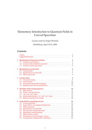
  • 14. The series (27) contains the singular term π 2 α−2 , a finite term, and further terms that vanish as α → 0. The crucial fact is that the singular term in Eq. (27) does not depend on L. (This would not have happened if we chose the cutoff e.g. as e−nα .) The limit L → ∞ in Eq. (25) is taken before the limit α → 0, so the divergent term π 2 α−2 cancels and the renormalized value of ∆ε is finite, ∆εren(L) = lim α→0 ε0 (L; α) − lim L→∞ ε0 (L; α) = − π 24L2 . (28) The formula (28) is the main result of this chapter; the zero-point energy density is nonzero in the presence of plates at x = 0 and x = L. The Casimir force between the plates is F = − d dL ∆E = − d dL (L∆εren) = − π 24L2 . Since the force is negative, the plates are pulled toward each other. Remark: negative energy. Note that the zero-point energy density (28) is negative. Quantum field theory generally admits quantum states with a negative expectation value of energy. 4 Oscillator with varying frequency A gravitational background influences quantum fields in such a way that the fre- quencies ωk of the modes become time-dependent, ωk(t). We shall examine this situation in detail in chapter 5. For now, let us consider a single harmonic oscilla- tor with a time-dependent frequency ω(t). 4.1 Quantization In the classical theory, the coordinate q(t) satisfies ¨q + ω2 (t)q = 0. (29) An important example of a function ω(t) is shown Fig. 1. The frequency is approx- imately constant except for a finite time interval, for instance ω ≡ ω0 for t ≤ t0 and ω ≡ ω1 for t ≥ t1. It is usually impossible to find an exact solution of Eq. (29) in such cases (of course, an approximate solution can be found numerically). How- ever, the solutions in the regimes t ≤ t0 and t ≥ t1 are easy to obtain: q(t) = Aeiω0t + Be−iω0t , t ≤ t0; q(t) = Aeiω1t + Be−iω1t , t ≥ t1. We shall be interested only in describing the behavior of the oscillator in these two regimes5 which we call the “in” and “out” regimes. The classical equation of motion (29) can be derived from the Lagrangian L (t, q, ˙q) = 1 2 ˙q2 − 1 2 ω(t)2 q2 . The corresponding canonical momentum is p = ˙q, and the Hamiltonian is H(p, q) = p2 2 + ω2 (t) q2 2 , (30) 5In the physics literature, the word regime stands for “an interval of values for a variable.” It should be clear from the context which interval for which variable is implied. 14
  • 15. ω(t) ω1 ω0 t0 t1 t Figure 1: A frequency function ω(t) with “in” and “out” regimes (at t ≤ t0 and t ≥ t1). which depends explicitly on the time t. Therefore, we do not expect that energy is conserved in this system. (There is an external agent that drives ω(t) and may exchange energy with the oscillator.) A time-dependent oscillator can be quantized using the technique of creation and annihilation operators. By analogy with Eq. (6), we try the ansatz ˆq(t) = 1 √ 2 v(t)ˆa+ + v∗ (t)ˆa− , ˆp(t) = 1 √ 2 ˙v(t)ˆa+ + ˙v∗ (t)ˆa− , (31) where v(t) is a complex-valued function that replaces eiωt , while the operators ˆa± are time-independent. The present task is to choose the function v(t) and the operators ˆa± in an appropriate way. We call v(t) the mode function because we shall later apply the same decomposition to modes of a quantum field. Since ˆq(t) must be a solution of Eq. (29), we find that v(t) must satisfy the same equation, ¨v + ω2 (t)v = 0. (32) Furthermore, the canonical commutation relation [ˆq(t), ˆp(t)] = i entails ˆa− , ˆa+ = 2i ˙vv∗ − ˙v∗v . Note that the expression ˙vv∗ − ˙v∗ v ≡ W[v, v∗ ] is the Wronskian of the solutions v(t) and v∗ (t), and it is well known that W = const. We may therefore normalize the mode function v(t) such that W[v, v∗ ] = ˙vv∗ − ˙v∗ v = 2i, (33) which will yield the standard commutation relations for ˆa± , ˆa− , ˆa+ = 1. We can then postulate the existence of the ground state |0 such that ˆa− |0 = 0. Excited states |n (n = 1, 2, ...) are defined in the standard way by Eq. (8). With the normalization (33), the creation and annihilation operators are ex- pressed through the canonical variables as ˆa− ≡ ˙v(t)ˆq(t) − v(t)ˆp(t) i √ 2 , ˆa+ ≡ − ˙v∗ (t)ˆq(t) − v∗ (t)ˆp(t) i √ 2 . (34) (Note that the l.h.s. of Eq. (34) are time-independent because the corresponding r.h.s. are Wronskians.) In this way, a choice of the mode function v(t) defines the operators ˆa± and the states |0 , |1 , ... 15
  • 16. It is clear that different choices of v(t) will in general define different operators ˆa± and different states |0 , |1 , ... It is not clear, a priori, which choice of v(t) cor- responds to the “correct” ground state of the oscillator. The choice of v(t) will be studied in the next section. Properties of mode functions Here is a summary of some elementary properties of a time-dependent oscillator equation ¨x + ω2 (t)x = 0. (35) This equation has a two-dimensional space of solutions. Any two linearly independent solutions x1(t) and x2(t) are a basis in that space. The expression W [x1, x2] ≡ ˙x1x2 − x1 ˙x2 is called the Wronskian of the two functions x1(t) and x2(t). It is easy to see that the Wronskian W [x1, x2] is time-independent if x1,2(t) satisfy Eq. (35). Moreover, W [x1, x2] = 0 if and only if x1(t) and x2(t) are two linearly independent solutions. If {x1(t), x2(t)} is a basis of solutions, it is convenient to define the complex func- tion v(t) ≡ x1(t) + ix2(t). Then v(t) and v∗ (t) are linearly independent and form a basis in the space of complex solutions of Eq. (35). It is easy to check that Im(˙vv∗ ) = ˙vv∗ − ˙v∗ v 2i = 1 2i W [v, v∗ ] = −W [x1, x2] = 0, and thus the quantity Im(˙vv∗ ) is a nonzero real constant. If v(t) is multiplied by a constant, v(t) → λv(t), the Wronskian W [v, v∗ ] changes by the factor |λ|2 . Therefore we may normalize v(t) to a prescribed value of Im(˙vv∗ ) by choosing the constant λ, as long as v and v∗ are linearly independent solutions so that W [v, v∗ ] = 0. A complex solution v(t) of Eq. (35) is an admissible mode function if v(t) is nor- malized by the condition Im(˙vv∗ ) = 1. It follows that any solution v(t) normalized by Im(˙vv∗ ) = 1 is necessarily complex-valued and such that v(t) and v∗ (t) are a basis of linearly independent complex solutions of Eq. (35). 4.2 Choice of mode function We have seen that different choices of the mode function v(t) lead to different defi- nitions of the operators ˆa± and thus to different “canditate ground states” |0 . The true ground state of the oscillator is the lowest-energy state and not merely some state |0 satisfying ˆa− |0 = 0, where ˆa− is some arbitrary operator. Therefore we may try to choose v(t) such that the mean energy 0| ˆH |0 is minimized. For any choice of the mode function v(t), the Hamiltonian is expressed through the operators ˆa± as ˆH = |˙v| 2 + ω2 |v| 2 4 2ˆa+ ˆa− + 1 + ˙v2 + ω2 v2 4 ˆa+ ˆa+ + ˙v∗2 + ω2 v∗2 4 ˆa− ˆa− . (36) Derivation of Eq. (36) In the canonical variables, the Hamiltonian is ˆH = 1 2 ˆp2 + 1 2 ω2 (t)ˆq2 . Now we expand the operators ˆp, ˆq through the mode functions using Eq. (31) and the commutation relation ˆ ˆa+ , ˆa− ˜ = 1. For example, the term ˆp2 gives ˆp2 = 1 √ 2 ` ˙v(t)ˆa+ + ˙v∗ (t)ˆa−´ 1 √ 2 ` ˙v(t)ˆa+ + ˙v∗ (t)ˆa−´ = 1 2 ` ˙v2 ˆa+ ˆa+ + ˙v ˙v∗ ` 2ˆa+ ˆa− + 1 ´ + ˙v∗2 ˆa− ˆa−´ . 16
  • 17. The term ˆq2 gives ˆq2 = 1 √ 2 ` v(t)ˆa+ + v∗ (t)ˆa− ´ 1 √ 2 ` v(t)ˆa+ + v∗ (t)ˆa− ´ = 1 2 ` v2 ˆa+ ˆa+ + vv∗ ` 2ˆa+ ˆa− + 1 ´ + v∗2 ˆa− ˆa− ´ . After some straightforward algebra we obtain the required result. It is easy to see from Eq. (36) that the mean energy at time t is given by E(t) ≡ 0| ˆH(t) |0 = | ˙v(t)| 2 + ω2 (t) |v(t)| 2 4 . (37) We would like to find the mode function v(t) that minimizes the above quantity. Note that E(t) is time-dependent, so we may first try to minimize E(t0) at a fixed time t0. The choice of the mode function v(t) may be specified by a set of initial condi- tions at t = t0, v(t0) = q, ˙v(t0) = p, where the parameters p and q are complex numbers satisfying the normalization constraint which follows from Eq. (33), q∗ p − p∗ q = 2i. (38) Now we need to find such p and q that minimize the expression |p| 2 + ω2 (t0) |q| 2 . This is a straightforward exercise (see below) which yields, for ω(t0) > 0, the fol- lowing result: v(t0) = 1 ω(t0) , ˙v(t0) = i ω(t0) = iω(t0)v(t0). (39) If, on the other hand, ω2 (t0) < 0 (i.e. ω is imaginary), there is no minimum. For now, we shall assume that ω(t0) is real. Then the mode function satisfying Eq. (39) will define the operators ˆa± and the state |t0 0 such that the instantaneous energy E(t0) has the lowest possible value Emin = 1 2 ω(t0). The state |t0 0 is called the instantaneous ground state at time t = t0. Derivation of Eq. (39) If some p and q minimize |p|2 + ω2 |q|2 , then so do eiλ p and eiλ q for arbitrary real λ; this is the freedom of choosing the overall phase of the mode function. We may choose this phase to make q real and write p = p1 + ip2 with real p1,2. Then Eq. (38) yields q = 2i p − p∗ = 1 p2 ⇒ 4E(t0) = p2 1 + p2 2 + ω2 (t0) p2 2 . (40) If ω2 (t0) > 0, the function E (p1, p2) has a minimum with respect to p1,2 at p1 = 0 and p2 = p ω(t0). Therefore the desired initial conditions for the mode function are given by Eq. (39). On the other hand, if ω2 (t0) < 0 the function Ek in Eq. (40) has no minimum because the expression p2 2 + ω2 (t0)p−2 2 varies from −∞ to +∞. In that case the instan- taneous lowest-energy ground state does not exist. 4.3 “In” and “out” states Let us now consider the frequency function ω(t) shown in Fig. 1. It is easy to see that the lowest-energy state is given by the mode function vin(t) = eiω0t in the “in” regime (t ≤ t0) and by vout(t) = eiω1t in the “out” regime (t ≥ t1). However, 17
  • 18. note that vin(t) = eiω0t for t > t0; instead, vin(t) is a solution of Eq. (29) with the initial conditions (39) at t = t0. Similarly, vout(t) = eiω1t for t < t1. While exact solutions for vin(t) and vout(t) are in general not available, we may still analyze the relationship between these solutions in the “in” and “out” regimes. Since the solutions e±iω1t are a basis in the space of solutions of Eq. (35), we may write vin(t) = αvout(t) + βv∗ out(t), (41) where α and β are time-independent constants. The relationship (41) between the mode functions is an example of a Bogolyubov transformation (see Sec. 2.2). Us- ing Eq. (33) for vin(t) and vout(t), it is straightforward to derive the property |α| 2 − |β| 2 = 1. (42) For a general ω(t), we will have β = 0 and hence there will be no single mode function v(t) matching both vin(t) and vout(t). Each choice of the mode function v(t) defines the corresponding creation and annihilation operators ˆa± . Let us denote by ˆa± in the operators defined using the mode function vin(t) and vout(t), respectively. It follows from Eqs. (34) and (41) that ˆa− in = αˆa− out − βˆa+ out. The inverse relation is easily found using Eq. (42), ˆa− out = α∗ ˆa− in + βˆa+ in. (43) Since generally β = 0, we cannot define a single set of operators ˆa± which will define the ground state |0 for all times. Moreover, in the intermediate regime where ω(t) is not constant, an instanta- neous ground state |t0 defined at time t will, in general, not be a ground state at the next moment, t + ∆t. Therefore, such a state |t0 cannot be trusted as a phys- ically motivated ground state. However, if we restrict our attention only to the “in” regime, the mode function vin(t) defines a perfectly sensible ground state |0in which remains the ground state for all t ≤ t0. Similarly, the mode function vout(t) defines the ground state |0out . Since we are using the Heisenberg picture, the quantum state |ψ of the oscil- lator is time-independent. It is reasonable to plan the following experiment. We prepare the oscillator in its ground state |ψ = |0in at some early time t < t0 within the “in” regime. Then we let the oscillator evolve until the time t = t1 and compare its quantum state (which remains |0in ) with the true ground state, |0out , at time t > t1 within the “out” regime. In the “out” regime, the state |0in is not the ground state any more, and thus it must be a superposition of the true ground state |0out and the excited states |nout defined using the “out” creation operator ˆa+ out, |nout = 1 √ n! ˆa+ out n |0out , n = 0, 1, 2, ... It can be easily verified that the vectors |nout are eigenstates of the Hamiltonian for t ≥ t1 (but not for t < t1): ˆH(t) |nout = ω1 n + 1 2 |nout , t ≥ t1. Similarly, the excited states |nin may be defined through the creation operator ˆa+ in. The states |nin are interpreted as n-particle states of the oscillator for t ≤ t0, while for t ≥ t1 the n-particle states are |nout . 18
  • 19. Remark: interpretation of the “in” and “out” states. We are presently working in the Heisenberg picture where quantum states are time-independent and operators depend on time. One may prepare the oscillator in a state |ψ , and the state of the oscillator re- mains the same throughout all time t. However, the physical interpretation of this state changes with time because the state |ψ is interpreted with help of the time-dependent operators ˆH(t), ˆa− (t), etc. For instance, we found that at late times (t ≥ t1) the vector |0in is not the lowest-energy state any more. This happens because the energy of the system changes with time due to the external force that drives ω(t). Without this force, we would have ˆa− in = ˆa− out and the state |0in would describe the physical vacuum at all times. 4.4 Relationship between “in” and “out” states The states |nout , where n = 0, 1, 2, ..., form a complete basis in the Hilbert space of the harmonic oscillator. However, the set of states |nin is another complete basis in the same space. Therefore the vector |0in must be expressible as a linear combination of the “out” states, |0in = ∞ n=0 Λn |nout , (44) where Λn are suitable coefficients. If the mode functions are related by a Bo- golyubov transformation (41), one can show that these coefficients Λn are given by Λ2n = 1 − β α 2 1/4 β α n (2n − 1)!! (2n)!! , Λ2n+1 = 0. (45) The relation (44) shows that the early-time ground state is a superposition of excited states at late times, having the probability |Λn| 2 for the occupation number n. We thus conclude that the presence of an external influence leads to excitations of the oscillator. (Later on, when we consider field theory, such excitations will be interpreted as particle production.) In the present case, the influence of external forces on the oscillator consists of the changing frequency ω(t), which is formally a parameter of the Lagrangian. For this reason, the excitations arising in a time- dependent oscillator are called parametric excitations. Finally, let us compute the expected particle number in the “out” regime, as- suming that the oscillator is in the state |0in . The expectation value of the number operator ˆNout ≡ ˆa+ outˆa− out in the state |0in is easily found using Eq. (43): 0in| ˆa+ outˆa− out |0in = 0in| αˆa+ in + β∗ ˆa− in α∗ ˆa− in + βˆa+ in |0in = |β| 2 . Therefore, a nonzero coefficient β signifies the presence of particles in the “out” region. Derivation of Eq. (45) In order to find the coefficients Λn, we need to solve the equation 0 = ˆa− in |0in = ` αˆa− out − βˆa+ out ´ ∞X n=0 Λn |nout . Using the known properties ˆa+ |n = √ n + 1 |n + 1 , ˆa− |n = √ n |n − 1 , we obtain the recurrence relation Λn+2 = Λn β α r n + 1 n + 2 ; Λ1 = 0. 19
  • 20. Therefore, only even-numbered Λ2n are nonzero and may be expressed through Λ0 as follows, Λ2n = Λ0 „ β α «n s 1 · 3 · ... · (2n − 1) 2 · 4 · ... · (2n) ≡ Λ0 „ β α «n s (2n − 1)!! (2n)!! , n ≥ 1. For convenience, one defines (−1)!! = 1, so the above expression remains valid also for n = 0. The value of Λ0 is determined from the normalization condition, 0in| 0in = 1, which can be rewritten as |Λ0|2 ∞X n=0 ˛ ˛ ˛ ˛ β α ˛ ˛ ˛ ˛ 2n (2n − 1)!! (2n)!! = 1. The infinite sum can be evaluated as follows. Let f(z) be an auxiliary function defined by the series f(z) ≡ ∞X n=0 z2n (2n − 1)!! (2n)!! . At this point one can guess that this is a Taylor expansion of f(z) = ` 1 − z2 ´−1/2 ; then one obtains Λ0 = 1/ p f(z) with z ≡ |β/α|. If we would like to avoid guessing, we could manipulate the above series in order to derive a differential equation for f(z): f(z) = 1 + ∞X n=1 z2n 2n − 1 2n (2n − 3)!! (2n − 2)!! = 1 + ∞X n=1 z2n (2n − 3)!! (2n − 2)!! − ∞X n=1 z2n 2n (2n − 3)!! (2n − 2)!! = 1 + z2 f(z) − ∞X n=1 z2n 2n (2n − 3)!! (2n − 2)!! . Taking d/dz of both parts, we have d dz ˆ 1 + z2 f(z) − f(z) ˜ = ∞X n=1 z2n−1 (2n − 3)!! (2n − 2)!! = zf(z), hence f(z) satisfies d dz ˆ (z2 − 1)f(z) ˜ = ` z2 − 1 ´ df dz + 2zf(z) = zf(z); f(0) = 1. The solution is f(z) = 1 √ 1 − z2 . Substituting z ≡ |β/α|, we obtain the required result, Λ0 = " 1 − ˛ ˛ ˛ ˛ β α ˛ ˛ ˛ ˛ 2 #1/4 . 4.5 Quantum-mechanical analogy The time-dependent oscillator equation (35) is formally similar to the stationary Schrödinger equation for the wave function ψ(x) of a quantum particle in a one- dimensional potential V (x), d2 ψ dx2 + (E − V (x)) ψ = 0. The two equations are related by the replacements t → x and ω2 (t) → E − V (x). 20
  • 21. x1 x2 incoming R T V (x) x Figure 2: Quantum-mechanical analogy: motion in a potential V (x). To illustrate the analogy, let us consider the case when the potential V (x) is almost constant for x < x1 and for x > x2 but varies in the intermediate region (see Fig. 2). An incident wave ψ(x) = exp(−ipx) comes from large positive x and is scattered off the potential. A reflected wave ψR(x) = R exp(ipx) is produced in the region x > x2 and a transmitted wave ψT (x) = T exp(−ipx) in the region x < x1. For most potentials, the reflection amplitude R is nonzero. The conservation of probability gives the constraint |R| 2 + |T | 2 = 1. The wavefunction ψ(x) behaves similarly to the mode function v(t) in the case when ω(t) is approximately constant at t ≤ t0 and at t ≥ t1. If the wavefunction represents a pure incoming wave x < x1, then at x > x2 the function ψ(x) will be a superposition of positive and negative exponents exp (±ikx). This is the phe- nomenon known as over-barrier reflection: there is a small probability that the particle is reflected by the potential, even though the energy is above the height of the barrier. The relation between R and T is similar to the normalization condition (42) for the Bogolyubov coefficients. The presence of the over-barrier reflection (R = 0) is analogous to the presence of particles in the “out” region (β = 0). 5 Scalar field in expanding universe Let us now turn to the situation when quantum fields are influenced by strong gravitational fields. In this chapter, we use units where c = G = 1, where G is Newton’s constant. 5.1 Curved spacetime Einstein’s theory of gravitation (General Relativity) is based on the notion of curved spacetime, i.e. a manifold with arbitrary coordinates x ≡ {xµ } and a met- ric gµν(x) which replaces the flat Minkowski metric ηµν. The metric defines the interval ds2 = gµνdxµ dxν , which describes physically measured lengths and times. According to the Einstein equation, the metric gµν(x) is determined by the distribution of matter in the entire universe. Here are some basic examples of spacetimes. In the absence of matter, the met- ric is equal to the Minkowski metric ηµν = diag (1, −1, −1, −1) (in Cartesian coor- dinates). In the presence of a single black hole of mass M, the metric can be written in spherical coordinates as ds2 = 1 − 2M r dt2 − 1 − 2M r −1 dr2 − r2 dθ2 + sin2 θdφ2 . 21
  • 22. Finally, a certain class of spatially homogeneous and isotropic distributions of mat- ter in the universe yields a metric of the form ds2 = dt2 − a2 (t) dx2 + dy2 + dy2 , (46) where a(t) is a certain function called the scale factor. (The interpretation is that a(t) “scales” the flat metric dx2 + dy2 + dz2 at different times.) Spacetimes with metrics of the form (46) are called Friedmann-Robertson-Walker (FRW) spacetimes with flat spatial sections (in short, flat FRW spacetimes). Note that it is only the three-dimensional spatial sections which are flat; the four-dimensional geometry of such spacetimes is usually curved. The class of flat FRW spacetimes is important in cosmology because its geometry agrees to a good precision with the present results of astrophysical measurements. In this course, we shall not be concerned with the task of obtaining the metric. It will be assumed that a metric gµν(x) is already known in some coordinates {xµ }. 5.2 Scalar field in cosmological background Presently, we shall study the behavior of a quantum field in a flat FRW spacetime with the metric (46). In Einstein’s General Relativity, every kind of energy influ- ences the geometry of spacetime. However, we shall treat the metric gµν(x) as fixed and disregard the influence of fields on the geometry. A minimally coupled, free, real, massive scalar field φ(x) in a curved spacetime is described by the action S = √ −gd4 x 1 2 gαβ (∂αφ) (∂βφ) − 1 2 m2 φ2 . (47) (Note the difference between Eq. (47) and Eq. (11): the Minkowski metric ηµν is replaced by the curved metric gµν, and the integration uses the covariant volume element √ −gd4 x. This is the minimal change necessary to make the theory of the scalar field compatible with General Relativity.) The equation of motion for the field φ is derived straightforwardly as gµν ∂µ∂νφ + 1 √ −g (∂νφ) ∂µ gµν√ −g + m2 φ = 0. (48) This equation can be rewritten more concisely using the covariant derivative cor- responding to the metric gµν, gµν ∇µ∇νφ + m2 φ = 0, which shows explicitly that this is a generalization of the Klein-Gordon equation to curved spacetime. We cannot directly use the quantization technique developed for fields in the flat spacetime. First, let us carry out a few mathematical transformations to sim- plify the task. The metric (46) for a flat FRW spacetime can be simplified if we replace the coordinate t by the conformal time η, η(t) ≡ t t0 dt a(t) , where t0 is an arbitrary constant. The scale factor a(t) must be expressed through the new variable η; let us denote that function again by a(η). In the coordinates (x, η), the interval is ds2 = a2 (η) dη2 − dx2 , (49) 22
  • 23. so the metric is conformally flat (equal to the flat metric multiplied by a factor): gµν = a2 ηµν, gµν = a−2 ηµν . Further, it is convenient to introduce the auxiliary field χ ≡ a(η)φ. Then one can show that the action (47) can be rewritten in terms of the field χ as follows, S = 1 2 d3 x dη χ′2 − (∇χ)2 − m2 eff(η)χ2 , (50) where the prime ′ denotes ∂/∂η, and meff is the time-dependent effective mass m2 eff(η) ≡ m2 a2 − a′′ a . (51) The action (50) is very similar to the action (11), except for the presence of the time-dependent mass. Derivation of Eq. (50) We start from Eq. (47). Using the metric (49), we have √ −g = a4 and gαβ = a−2 ηαβ . Then √ −g m2 φ2 = m2 a2 χ2 , √ −g gαβ φ,αφ,β = a2 ` φ′2 − (∇φ)2 ´ . Substituting φ = χ/a, we get a2 φ′2 = χ′2 − 2χχ′ a′ a + χ2 „ a′ a «2 = χ′2 + χ2 a′′ a − » χ2 a′ a –′ . The total time derivative term can be omitted from the action, and we obtain the re- quired expression. Thus, the dynamics of a scalar field φ in a flat FRW spacetime is mathematically equivalent to the dynamics of the auxiliary field χ in the Minkowski spacetime. All the information about the influence of gravitation on the field φ is encapsulated in the time-dependent mass meff(η) defined by Eq. (51). Note that the action (50) is explicitly time-dependent, so the energy of the field χ is generally not conserved. We shall see that in quantum theory this leads to the possibility of particle creation; the energy for new particles is supplied by the gravitational field. 5.3 Mode expansion It follows from the action (50) that the equation of motion for χ(x, η) is χ′′ − ∆χ + m2 a2 − a′′ a χ = 0. (52) Expanding the field χ in Fourier modes, χ (x, η) = d3 k (2π)3/2 χk(η)eik·x , (53) we obtain from Eq. (52) the decoupled equations of motion for the modes χk(η), χ′′ k + k2 + m2 a2 (η) − a′′ a χk ≡ χ′′ k + ω2 k(η)χk = 0. (54) All the modes χk(η) with equal |k| = k are complex solutions of the same equa- tion (54). This equation describes a harmonic oscillator with a time-dependent frequency. Therefore, we may apply the techniques we developed in chapter 4. 23
  • 24. We begin by choosing a mode function vk(η), which is a complex-valued solu- tion of v′′ k + ω2 k(η)vk = 0, ω2 k(η) ≡ k2 + m2 eff(η). (55) Then, the general solution χk(η) is expressed as a linear combination of vk and v∗ k as χk(η) = 1 √ 2 a− k v∗ k(η) + a+ −kvk(η) , (56) where a± k are complex constants of integration that depend on the vector k (but not on η). The index −k in the second term of Eq. (56) and the factor 1√ 2 are chosen for later convenience. Since χ is real, we have χ∗ k = χ−k. It follows from Eq. (56) that a+ k = a− k ∗ . Combining Eqs. (53) and (56), we find χ (x, η) = d3 k (2π)3/2 1 √ 2 a− k v∗ k(η) + a+ −kvk(η) eik·x = d3 k (2π)3/2 1 √ 2 a− k v∗ k(η)eik·x + a+ k vk(η)e−ik·x . (57) Note that the integration variable k was changed (k → −k) in the second term of Eq. (57) to make the integrand a manifestly real expression. (This is done only for convenience.) The relation (57) is called the mode expansion of the field χ (x, η) w.r.t. the mode functions vk(η). At this point the choice of the mode functions is still arbi- trary. The coefficients a± k are easily expressed through χk(η) and vk(η): a− k = √ 2 v′ kχk − vkχ′ k v′ kv∗ k − vkv∗′ k = √ 2 W [vk, χk] W [vk, v∗ k] ; a+ k = a− k ∗ . (58) Note that the numerators and denominators in Eq. (58) are time-independent since they are Wronskians of solutions of the same oscillator equation. 5.4 Quantization of scalar field The field χ(x) can be quantized directly through the mode expansion (57), which can be used for quantum fields in the same way as for classical fields. The mode expansion for the field operator ˆχ is found by replacing the constants a± k in Eq. (57) by time-independent operators ˆa± k : ˆχ (x, η) = d3 k (2π)3/2 1 √ 2 eik·x v∗ k(η)ˆa− k + e−ik·x vk(η)ˆa+ k , (59) where vk(η) are mode functions obeying Eq. (55). The operators ˆa± k satisfy the usual commutation relations for creation and annihilation operators, ˆa− k , ˆa+ k′ = δ(k − k′ ), ˆa− k , ˆa− k′ = ˆa+ k , ˆa+ k′ = 0. (60) The commutation relations (60) are consistent with the canonical relations [χ(x1, η), χ′ (x2, η)] = iδ(x1 − x2) only if the mode functions vk(η) are normalized by the condition Im (v′ kv∗ k) = v′ kv∗ k − vkv′∗ k 2i ≡ W [vk, v∗ k] 2i = 1. (61) 24
  • 25. Therefore, quantization of the field ˆχ can be accomplished by postulating the mode expansion (59), the commutation relations (60) and the normalization (61). The choice of the mode functions vk(η) will be made later on. The mode expansion (59) can be visualized as the general solution of the field equation (52), where the operators ˆa± k are integration constants. The mode expan- sion can also be viewed as a definition of the operators ˆa± k through the field operator ˆχ (x, η). Explicit formulae relating ˆa± k to ˆχ and ˆπ ≡ ˆχ′ are analogous to Eq. (58). Clearly, the definition of ˆa± k depends on the choice of the mode functions vk(η). 5.5 Vacuum state and particle states Once the operators ˆa± k are determined, the vacuum state |0 is defined as the eigen- state of all annihilation operators ˆa− k with eigenvalue 0, i.e. ˆa− k |0 = 0 for all k. An excited state |mk1 , nk2 , ... with the occupation numbers m, n, ... in the modes χk1 , χk2 , ..., is constructed by |mk1 , nk2 , ... ≡ 1 √ m!n!... ˆa+ k1 m ˆa+ k2 n ... |0 . (62) We write |0 instead of |0k1 , 0k2 , ... for brevity. An arbitrary quantum state |ψ is a linear combination of these states, |ψ = m,n,... Cmn... |mk1 , nk2 , ... . If the field is in the state |ψ , the probability for measuring the occupation number m in the mode χk1 , the number n in the mode χk2 , etc., is |Cmn...| 2 . Let us now comment on the role of the mode functions. Complex solutions vk(η) of a second-order differential equation (55) with one normalization condi- tion (61) are parametrized by one complex parameter. Multiplying vk(η) by a con- stant phase eiα introduces an extra phase e±iα in the operators ˆa± k , which can be compensated by a constant phase factor eiα in the state vectors |0 and |mk1 , nk2 , ... . There remains one real free parameter that distinguishes physically inequivalent mode functions. With each possible choice of the functions vk(η), the operators ˆa± k and consequently the vacuum state and particle states are different. As long as the mode functions satisfy Eqs. (55) and (61), the commutation relations (60) hold and thus the operators ˆa± k formally resemble the creation and annihilation operators for particle states. However, we do not yet know whether the operators ˆa± k obtained with some choice of vk(η) actually correspond to physical particles and whether the quantum state |0 describes the physical vacuum. The correct commutation relations alone do not guarantee the validity of the physical interpretation of the operators ˆa± k and of the state |0 . For this interpretation to be valid, the mode func- tions must be appropriately selected; we postpone the consideration of this important issue until Sec. 5.8 below. For now, we shall formally study the consequences of choosing several sets of mode functions to quantize the field φ. 5.6 Bogolyubov transformations Suppose two sets of isotropic mode functions uk(η) and vk(η) are chosen. Since uk and u∗ k are a basis, the function vk is a linear combination of uk and u∗ k, e.g. v∗ k(η) = αku∗ k(η) + βkuk(η), (63) with η-independent complex coefficients αk and βk. If both sets vk(η) and uk(η) are normalized by Eq. (61), it follows that the coefficients αk and βk satisfy |αk|2 − |βk|2 = 1. (64) 25
  • 26. In particular, |αk| ≥ 1. Derivation of Eq. (64) We suppress the index k for brevity. The normalization condition for u(η) is u∗ u′ − uu′∗ = 2i. Expressing u through v as given, we obtain ` |α|2 − |β|2´ ` v∗ v′ − vv′∗´ = 2i. The formula (64) follows from the normalization of v(η). Using the mode functions uk(η) instead of vk (η), one obtains an alternative mode expansion which defines another set ˆb± k of creation and annihilation opera- tors, ˆχ (x, η) = d3 k (2π)3/2 1 √ 2 eik·x u∗ k(η)ˆb− k + e−ik·x uk(η)ˆb+ k . (65) The expansions (59) and (65) express the same field ˆχ (x, η) through two different sets of functions, so the k-th Fourier components of these expansions must agree, eik·x u∗ k(η)ˆb− k + uk(η)ˆb+ −k = eik·x v∗ k(η)ˆa− k + vk(η)ˆa+ −k . A substitution of vk through uk using Eq. (63) gives the following relation between the operators ˆb± k and ˆa± k : ˆb− k = αkˆa− k + β∗ k ˆa+ −k, ˆb+ k = α∗ kˆa+ k + βkˆa− −k. (66) The relation (66) and the complex coefficients αk, βk are called respectively the Bogolyubov transformation and the Bogolyubov coefficients.6 The two sets of annihilation operators ˆa− k and ˆb− k define the corresponding vacua (a)0 and (b)0 , which we call the “a-vacuum” and the “b-vacuum.” Two parallel sets of excited states are built from the two vacua using Eq. (62). We refer to these states as a-particle and b-particle states. So far the physical interpretation of the a- and b-particles remains unspecified. Later on, we shall apply this for- malism to study specific physical effects and the interpretation of excited states corresponding to various mode functions will be explained. At this point, let us only remark that the b-vacuum is in general a superposition of a-states, similarly to what we found in Sec. 4.4. 5.7 Mean particle number Let us calculate the mean number of b-particles of the mode χk in the a-vacuum state. The expectation value of the b-particle number operator ˆN (b) k = ˆb+ k ˆb− k in the state (a)0 is found using Eq. (66): (a)0 ˆN(b) (a)0 = (a)0 ˆb+ k ˆb− k (a)0 = (a)0 α∗ kˆa+ k + βkˆa− −k αkˆa− k + β∗ k ˆa+ −k (a)0 = (a)0 βkˆa− −k β∗ k ˆa+ −k (a)0 = |βk| 2 δ(3) (0). (67) The divergent factor δ(3) (0) is a consequence of considering an infinite spatial vol- ume. This divergent factor would be replaced by the box volume V if we quantized the field in a finite box. Therefore we can divide by this factor and obtain the mean density of b-particles in the mode χk, nk = |βk|2 . (68) 6The pronunciation is close to the American “bogo-lube-of” with the third syllable stressed. 26
  • 27. The Bogolyubov coefficient βk is dimensionless and the density nk is the mean number of particles per spatial volume d3 x and per wave number d3 k, so that nkd3 k d3 x is the (dimensionless) total mean number of b-particles in the a-vacuum state. The combined mean density of particles in all modes is d3 k |βk| 2 . Note that this integral might diverge, which would indicate that one cannot disregard the backreaction of the produced particles on other fields and on the metric. 5.8 Instantaneous lowest-energy vacuum In the theory developed so far, the particle interpretation depends on the choice of the mode functions. For instance, the a-vacuum (a)0 defined above is a state without a-particles but with b-particle density nk in each mode χk. A natural ques- tion to ask is whether the a-particles or the b-particles are the correct representation of the observable particles. The problem at hand is to determine the mode func- tions that describe the “actual” physical vacuum and particles. Previously, we defined the vacuum state as the eigenstate with the lowest en- ergy. However, in the present case the Hamiltonian explicitly depends on time and thus does not have time-independent eigenstates that could serve as vacuum states. One possible prescription for the vacuum state is to select a particular moment of time, η = η0, and to define the vacuum |η0 0 as the lowest-energy eigenstate of the instantaneous Hamiltonian ˆH(η0). To obtain the mode functions that describe the vacuum |η0 0 , we first compute the expectation value (v)0 ˆH(η0) (v)0 in the vacuum state (v)0 determined by arbitrarily chosen mode functions vk(η). Then we can minimize that expectation value with respect to all possible choices of vk(η). (A standard result in linear algebra is that the minimization of x| ˆA |x with respect to all normalized vectors |x is equivalent to finding the eigenvector |x of the operator ˆA with the smallest eigenvalue.) This computation is analogous to that of Sec. 4.2, and the result is similar to Eq. (39): If ω2 k(η0) > 0, the required initial conditions for the mode functions are vk (η0) = 1 ωk(η0) , v′ k(η0) = i ωk(η0) = iωkvk(η0). (69) If ω2 k(η0) < 0, the instantaneous lowest-energy vacuum state does not exist. For a scalar field in the Minkowski spacetime, ωk is time-independent and the prescription (69) yields the standard mode functions vk(η) = 1 √ ωk eiωkη , which remain the vacuum mode functions at all times. But this is not the case for a time-dependent gravitational background, because then ωk(η) = const and the mode function selected by the initial conditions (69) imposed at a time η0 will generally differ from the mode function selected at another time η1 = η0. In other words, the state |η0 0 is not an energy eigenstate at time η1. In fact, one can show that there are no states which remain instantaneous eigenstates of the Hamiltonian at all times. 5.9 Computation of Bogolyubov coefficients Computations of Bogolyubov coefficients requires knowledge of solutions of Eq. (55), which is an equation of a harmonic oscillator with a time-dependent frequency, 27
  • 28. with specified initial conditions. Suppose that vk(η) and uk(η) are mode functions describing instantaneous lowest-energy states defined at times η = η0 and η = η1. To determine the Bogolyubov coefficients αk and βk connecting these mode func- tions, it is necessary to know the functions vk(η) and uk(η) and their derivatives at only one value of η, e.g. at η = η0. From Eq. (63) and its derivative at η = η0, we find v∗ k (η0) = αku∗ k (η0) + βkuk (η0) , v∗′ k (η0) = αku∗′ k (η0) + βku′ k (η0) . This system of equations can be solved for αk and βk using Eq. (61): αk = u′ kv∗ k − ukv∗′ k 2i η0 , β∗ k = u′ kvk − ukv′ k 2i η0 . (70) These relations hold at any time η0 (note that the numerators are Wronskians and thus are time-independent). For instance, knowing only the asymptotics of vk(η) and uk(η) at η → −∞ would suffice to compute αk and βk. A well-known method to obtain an approximate solution of equations of the type (55) is the WKB approximation, which gives the approximate solution satis- fying the condition (69) at time η = η0 as vk(η) ≈ 1 ωk(η) exp i η η0 ωk(η1)dη1 . (71) However, it is straightforward to see that the approximation (71) satisfies the in- stantaneous minimum-energy condition at every other time η = η0 as well. In other words, within the WKB approximation, uk(η) ≈ vk(η). Therefore, if we use the WKB approximation to compute the Bogolyubov coefficient between instan- taneous vacuum states, we shall obtain the incorrect result βk = 0. The WKB approximation is insufficiently precise to capture the difference between the in- stantaneous vacuum states defined at different times. One can use the following method to obtain a better approximation to the mode function vk(η). Let us focus attention on one mode and drop the index k. Introduce a new variable Z(η) instead of v(η) as follows, v(η) = 1 ω(η0) exp i η η0 ω(η1)dη1 + η η0 Z(η1)dη1 ; v′ v = iω(η) + Z(η). If ω(η) is a slow-changing function, then we expect that v(η) is everywhere approx- imately equal to 1√ ω exp i η ω(η)dη and the function Z(η) under the exponential is a small correction; in particular, Z(η0) = 0 at the time η0. It is straightforward to derive the equation for Z(η) from Eq. (55), Z′ + 2iωZ = −iω′ − Z2 . This equation can be solved using perturbation theory by treating Z2 as a small perturbation. To obtain the first approximation, we disregard Z2 and straightfor- wardly solve the resulting linear equation, which yields Z(1)(η) = −i η η0 dη1ω′ (η1) exp −2i η η1 ω(η2)dη2 . Note that Z(1)(η) is an integral of a slow-changing function ω′ (η) multiplied by a quickly oscillating function and is therefore small, |Z| ≪ ω. The first approxi- mation Z(1) is sufficiently precise in most cases. The resulting approximate mode 28
  • 29. function is v(η) ≈ 1 ω(η0) exp i η η0 ω(η1)dη1 + η η0 Z(1)(η)dη . The Bogolyubov coefficient β between instantaneous lowest-energy states defined at times η0 and η1 can be approximately computed using Eq. (70): u(η1) = 1 ω(η1) ; u′ (η1) = iω(η1)u(η1); β∗ = 1 2i ω(η1) [iω(η1)v(η1) − v′ (η1)] = v(η1) iω − v′ v η1 2i ω(η1) ≈ − v(η1)Z(η1) 2i ω(η1) . Since v(η1) is of order ω−1/2 and |Z| ≪ ω, the number of particles is small: |β| 2 ≪ 1. 6 Amplitude of quantum fluctuations In the previous chapter the focus was on particle production. The main observ- able of interest was the average particle number ˆN . Now we consider another important quantity—the amplitude of field fluctuations. 6.1 Fluctuations of averaged fields The value of a field cannot be observed at a mathematical point in space. Realis- tic devices can only measure the value of the field averaged over some region of space. Spatial averages are also the relevant quantity in cosmology because struc- ture formation in the universe is explained by fluctuations occurring over large regions, e.g. of galaxy size. Therefore, let us consider values of fields averaged over a spatial domain. A convenient way to describe spatial averaging over arbitrary domains is by using window functions. A window function for scale L is any function W(x) which is of order 1 for |x| L, rapidly decays for |x| ≫ L, and satisfies the nor- malization condition W (x) d3 x = 1. (72) A typical example of a window function is the spherical Gaussian window WL (x) = 1 (2π)3/2L3 exp − |x| 2 2L2 , which selects |x| L. This window can be used to describe measurements per- formed by a device that cannot resolve distances smaller than L. We define the averaged field operator ˆχL(η) by integrating the product of ˆχ(x, η) with a window function that selects the scale L, ˆχL(η) ≡ d3 x ˆχ (x, η) WL(x), where we used the Gaussian window (although the final result will not depend on this choice). The amplitude δχL(η) of fluctuations in ˆχL(η) in a quantum state |ψ is found from δχ2 L(η) ≡ ψ| [ˆχL(η)] 2 |ψ . 29
  • 30. For simplicity, we consider the vacuum state |ψ = |0 . Then the amplitude of vacuum fluctuations in ˆχL(η) can be computed as a function of L. We use the mode expansion (59) for the field operator ˆχ(x, η), assuming that the mode functions vk(η) are given. After some straightforward algebra we find 0| d3 x WL(x)ˆχ (x, η) 2 |0 = 1 2 d3 k (2π)3 |vk| 2 e−k2 L2 . Since the factor e−k2 L2 is of order 1 for |k| L−1 and almost zero for |k| L−1 , we can estimate the above integral as follows, 1 2 d3 k (2π)3 |vk|2 e−k2 L2 ∼ L−1 0 k2 |vk|2 dk ∼ k3 |vk|2 k=L−1 . Thus the amplitude of fluctuations δχL is (up to a factor of order 1) δχ2 L ∼ k3 |vk| 2 , where k ∼ L−1 . (73) The result (73) is (for any choice of the window function WL) an order-of- magnitude estimate of the amplitude of fluctuations on scale L. This quantity, which we denote by δχL(η), is defined only up to a factor of order 1 and is a func- tion of time η and of the scale L. Expressed through the wavenumber k ≡ 2πL−1 , the fluctuation amplitude is usually called the spectrum of fluctuations. 6.2 Fluctuations in Minkowski spacetime Let us now compute the spectrum of fluctuations for a scalar field in the Minkowski space. The vacuum mode functions are vk(η) = ω −1/2 k exp (iωkη), where ωk = √ k2 + m2. Thus, the spectrum of fluctuations in vacuum is δχL(η) = k3/2 |vk(η)| = k3/2 (k2 + m2) 1/4 . (74) This time-independent spectrum is sketched in Fig. 3. When measured with a high-resolution device (small L), the field shows large fluctuations. On the other hand, if the field is averaged over a large volume (L → ∞), the amplitude of fluctuations tends to zero. 6.3 de Sitter spacetime The de Sitter spacetime is used in cosmology to describe periods of accelerated expansion of the universe. The amplitude of fluctuations is an important quantity to compute in that context. The geometry of the de Sitter spacetime may be specified by a flat FRW metric ds2 = dt2 − a2 (t)dx2 (75) with the scale factor a(t) defined by a(t) = a0eHt . (76) The Hubble parameter H = ˙a/a > 0 is a fixed constant. For convenience, we redefine the origin of time t to set a0 = 1, so that a(t) = exp(Ht). The exponen- tially growing scale factor describes an accelerating expansion (inflation) of the universe. 30
  • 31. δχ k ∼ k ∼ k3/2 Figure 3: A sketch of the spectrum of fluctuations δχL in the Minkowski space; L ≡ 2πk−1 . (The logarithmic scaling is used for both axes.) Horizons An important feature of the de Sitter spacetime—the presence of horizons—is re- vealed by the following consideration of trajectories of lightrays. A null worldline x(t) satisfies a2 (t) ˙x2 (t) = 1, which yields the solution |x(t)| = 1 H e−Ht0 − e−Ht for trajectories starting at the origin, x(t0) = 0. Therefore all lightrays emitted at the origin at t = t0 asymptotically approach the sphere |x| = rmax(t0) ≡ H−1 exp(−Ht0) = (aH) −1 . This sphere is the horizon for the observer at the origin; the spacetime expands too quickly for lightrays to reach any points beyond the horizon. Similarly, observers at the origin will never receive any lightrays emitted at t = t0 at points |x| > rmax. It is easy to verify that at any time t0 the horizon is always at the same proper distance a(t0)rmax(t0) = H−1 from the observer. This distance is called the horizon scale. 6.4 Quantum fields in de Sitter spacetime To describe a real scalar field φ (x, t) in the de Sitter spacetime, we first transform the coordinate t to make the metric explicitly conformally flat: ds2 = dt2 − a2 (t)dx2 = a2 (η) dη2 − dx2 , where the conformal time η and the scale factor a(η) are η = − 1 H e−Ht , a(η) = − 1 Hη . The conformal time η changes from −∞ to 0 when the proper time t goes from −∞ to +∞. (Since the value of η is always negative, we shall sometimes have to write |η| in the equations. However, it is essential that the variable η grows when t grows, so we cannot use −η as the time variable. For convenience, we chose the origin of η so that the infinite future corresponds to η = 0.) 31
  • 32. The field φ(x, η) can now be quantized by the method of Sec. 2.2. We introduce the auxiliary field χ ≡ aφ and use the mode expansion (59)-(55) with ω2 k(η) = k2 + m2 a2 − a′′ a = k2 + m2 H2 − 2 1 η2 . (77) From this expression it is clear that the effective frequency may become imaginary, i.e. ω2 k(η) < 0, if m2 < 2H2 . In most cosmological scenarios where the early uni- verse is approximated by a region of the de Sitter spacetime, the relevant value of H is much larger than the masses of elementary particles, i.e. m ≪ H. Therefore, for simplicity we shall consider the massless field. 6.5 Bunch-Davies vacuum state As we saw before, the vacuum state of a field is determined by the choice of mode functions. Let us now find the appropriate mode functions for a scalar field in de Sitter spacetime. With the definition (77) of the effective frequency, where we set m = 0, Eq. (55) becomes v′′ k + k2 − 2 η2 vk = 0. (78) The general solution of Eq. (78) can be written as vk(η) = Ak 1 + i kη eikη + Bk 1 − i kη e−ikη , (79) where Ak and Bk are constants. It is straightforward to check that the normal- ization of the mode function, Im (v∗ kv′ k) = 1, constrains the constants Ak and Bk by |Ak| 2 − |Bk| = 1 k . The constants Ak, Bk determine the mode functions and must be chosen ap- propriately to obtain a physically motivated vacuum state. For fields in de Sitter spacetime, there is a preferred vacuum state, which is known as the Bunch-Davies (BD) vacuum. This state is defined essentially as the Minkowski vacuum in the early-time limit (η → −∞) of each mode. Before introducing the BD vacuum, let us consider the prescription of the in- stantaneous vacuum defined at a time η = η0. If we had ω2 k(η0) > 0 for all k, this prescription would yield a well-defined vacuum state. However, there always ex- ists a small enough k such that k |η0| ≪ 1 and thus ω2 k(η0) < 0. We have seen that the energy in a mode χk cannot be minimized when ω2 k < 0. Therefore the instan- taneous energy prescription cannot define a vacuum state of the entire quantum field (for all modes) but only for the modes χk with k |η0| 1. Note that these are the modes whose wavelength was shorter than the horizon length, (aH)−1 = |η0|, at time η0 (i.e. the subhorizon modes). The motivation for introducing the BD vacuum state is the following. The effec- tive frequency ωk(η) becomes constant in the early-time limit η → −∞. Physically, this means that the influence of gravity on each mode χk is negligible at sufficiently early (k-dependent) times. When gravity is negligible, there is a unique vacuum prescription—the Minkowski vacuum, which coincides with the instantaneous minimum-energy vacuum at all times. So it is natural to define the mode func- tions vk(η) by applying the Minkowski vacuum prescription in the limit η → −∞, separately for each mode χk. This prescription can be expressed by the asymptotic relations vk(η) → 1 √ ωk eiωkη , v′ k(η) vk(η) → iωk, as η → −∞. (80) 32
  • 33. The vacuum state determined by the mode functions vk(η) satisfying Eq. (80) is called the Bunch-Davies vacuum. It follows that the mode functions of the BD vacuum are given by Eq. (79) with Ak = 1/ √ k and Bk = 0, namely vk(η) = 1 √ k 1 + i kη eikη . (81) The Bunch-Davies vacuum prescription has important applications in cosmol- ogy where the de Sitter spacetime approximates the inflationary stage of the evo- lution of the universe. However, this approximation is valid only for a certain time interval, for instance ηi < η < ηf , while at earlier times, η < ηi, the spacetime is not de Sitter. Therefore the procedure of imposing the minimum-energy conditions at earlier times η < ηi cannot be justified, and the BD vacuum state can be used only for modes χk such that k |ηi| ≫ 1. However, it is these modes that are important for cosmological predictions. 6.6 Spectrum of fluctuations in the BD vacuum Let us now compute the fluctuation amplitude δφL(η) in the BD vacuum state and compare the result with the fluctuations in Minkowski spacetime. According to the formula (73), the amplitude of fluctuations is determined by absolute values of the mode functions. Up to now we have been mostly working with the auxiliary field ˆχ(x) = aˆφ(x). The mode expansion for ˆφ(x) is simply a−1 (η) times the mode expansion for ˆχ. Therefore, the mode functions of the field ˆφ are a−1 (η)vk(η), where vk(η) are the mode functions of the field ˆχ. Hence, the spectrum of fluctuations of ˆφ is δφL(η) = a−1 (η)k3/2 |vk(η)| = H k2η2 + 1. (82) This spectrum is to be compared with Eq. (74) with m = 0. The spectrum (82) for early times (|η| ≫ k) is the same as in the Minkowski spacetime, while for late times or for superhorizon scales (k ≪ |η| −1 ) the spectrum (82) becomes almost independent of k (scale-invariant) and shows much larger fluctuations than the spectrum (74). The growth of fluctuations is due to the influence of gravity on the field ˆφ. The growth of quantum fluctuations is used in cosmology to explain the for- mation of large-scale structures (galaxies and clusters of galaxies) in the early uni- verse. The theory of cosmological inflation assumes the existence of a de Sitter-like epoch in the history of the universe. During this epoch, vacuum fluctuations of the fields were significantly amplified. The resulting large quantum fluctuations acted as seeds for the inhomogeneities of energy density, which then grew by gravita- tional collapse and eventually caused the formation of galaxies. This theory is a practical application of quantum field theory in curved spacetime to astrophysics. 7 Unruh effect The Unruh effect predicts that particles will be detected in a vacuum by an acceler- ated observer. In this chapter we consider the simplest case, in which the observer moves with constant acceleration through Minkowski spacetime and measures the number of particles in a massless scalar field. Even though the field is in the vac- uum state, the observer finds a distribution of particles characteristic of a thermal bath of blackbody radiation. 33
  • 34. 7.1 Kinematics of uniformly accelerated motion First we consider the trajectory of an object moving with constant acceleration in the Minkowski spacetime. A model of this situation is a spaceship with an infinite energy supply and a propulsion engine that exerts a constant force (but moves with the ship). The resulting motion of the spaceship is such that the acceleration of the ship in its own frame of reference (the proper acceleration) is constant. This is the natural definition of a uniformly accelerated motion in a relativistic theory. (An object cannot move with dv/dt = const for all time because its velocity is always smaller than the speed of light, |v| < 1.) We now introduce the reference frames that will play a major role in our consid- erations: the laboratory frame, the proper frame, and the comoving frame. The lab- oratory frame is the usual inertial reference frame with the coordinates (t, x, y, z). The proper frame is the accelerated system of reference that moves together with the observer; we shall also call it the accelerated frame. The comoving frame de- fined at a time t0 is the inertial frame in which the accelerated observer is instan- taneously at rest at t = t0. (Thus the term comoving frame actually refers to a different frame for each t0.) By definition, the observer’s proper acceleration at time t = t0 is the 3-acceleration measured in the comoving frame at time t0. We consider a uniformly accelerated observer whose proper acceleration is time-independent and equal to a given 3- vector a. The trajectory of such an observer may be described by a worldline xµ (τ), where τ is the proper time measured by the observer. The proper time parametrization implies the condition uµ uµ = 1, uµ ≡ dxµ dτ . (83) It is a standard result that the 4-acceleration in the laboratory frame, aµ ≡ duµ dτ = d2 xµ dτ2 , is related to the three-dimensional proper acceleration a by aµ aµ = − |a| 2 . (84) Derivation of Eq. (84). Let uµ (τ) be the observer’s 4-velocity and let tc be the time variable in the comoving frame defined at τ = τ0; this is the time measured by an inertial observer moving with the constant velocity uµ (τ0). We shall show that the 4- acceleration aµ (τ) in the comoving frame has components ` 0, a1 , a2 , a3 ´ , where ai are the components of the acceleration 3-vector a ≡ d2 x/dt2 c measured in the comoving frame. It will then follow that Eq. (84) holds in the comoving frame, and hence it holds also in the laboratory frame since the Lorentz-invariant quantity aµ aµ is the same in all frames. Since the comoving frame moves with the velocity uµ (τ0), the 4-vector uµ (τ0) has the components (1, 0, 0, 0) in that frame. The derivative of the identity uµ (τ)uµ(τ) = 1 with respect to τ yields aµ (τ)uµ(τ) = 0, therefore a0 (τ0) = 0 in the comoving frame. Since dtc = u0 (τ)dτ and u0 (τ0) = 1, we have d2 xµ dt2 c = 1 u0 d dτ » 1 u0 dxµ dτ – = d2 xµ dτ2 + dxµ dτ d dτ 1 u0 . It remains to compute d dτ 1 u0(τ0) = − ˆ u0 (τ0) ˜−2 du0 dτ ˛ ˛ ˛ ˛ τ=τ0 = −a0 (τ0) = 0, 34
  • 35. and it follows that d2 xµ /dτ2 = d2 xµ /dt2 c = ` 0, a1 , a2 , a3 ´ as required. (Self-test ques- tion: why is aµ = duµ /dτ = 0 even though uµ = (1, 0, 0, 0) in the comoving frame?) We now derive the trajectory xµ (τ) of the accelerated observer. Without loss of generality, we may assume that the acceleration is parallel to the x axis, a ≡ (a, 0, 0), where a > 0, and that the observer moves only in the x direction. Then the coordinates y and z of the observer remain constant and only the functions x(τ), t(τ) need to be computed. From Eqs. (83)-(84) it is straightforward to derive the general solution x(τ) = x0 − 1 a + 1 a cosh aτ, t(τ) = t0 + 1 a sinh aτ. (85) This trajectory has zero velocity at τ = 0 (which implies x = x0, t = t0). Derivation of Eq. (85). Since aµ = duµ /dτ and u2 = u3 = 0, the components u0 , u1 of the velocity satisfy „ du0 dτ «2 − „ du1 dτ «2 = −a2 , ` u0 ´2 − ` u1 ´2 = 1. We may assume that u0 > 0 (the time τ grows together with t) and that du1 /dτ > 0, since the acceleration is in the positive x direction. Then u0 = q 1 + (u1)2 ; du1 dτ = a q 1 + (u1)2 . The solution with the initial condition u1 (0) = 0 is u1 (τ) ≡ dx dτ = sinh aτ, u0 (τ) ≡ dt dτ = cosh aτ. After an integration we obtain Eq. (85). The trajectory (85) has a simpler form if we choose the initial conditions x(0) = a−1 and t(0) = 0. Then the worldline is a branch of the hyperbola x2 −t2 = a−2 (see Fig. 4). At large |t| the worldline approaches the lightcone. The observer comes in from x = +∞, decelerates and stops at x = a−1 , and then accelerates back towards infinity. In the comoving frame of the observer, this motion takes infinite proper time, from τ = −∞ to τ = +∞. From now on, we drop the coordinates y and z and work in the 1+1-dimensional spacetime (t, x). 7.2 Coordinates in the proper frame To describe quantum fields as seen by an accelerated observer, we need to use the proper coordinates (τ, ξ), where τ is the proper time and ξ is the distance measured by the observer. The proper coordinate system (τ, ξ) is related to the laboratory frame (t, x) by some transformation functions τ(t, x) and ξ(t, x) which we shall now determine. The observer’s trajectory t(τ), x(τ) should correspond to the line ξ = 0 in the proper coordinates. Let the observer hold a rigid measuring stick of proper length ξ0, so that the entire stick accelerates together with the observer. Then the stick is instantaneously at rest in the comoving frame and the far endpoint of the stick has the proper coordinates (τ, ξ0) at time τ. We shall derive the relation between the coordinates (t, x) and (τ, ξ) by computing the laboratory coordinates (t, x) of the far end of the stick as functions of τ and ξ0. 35
  • 36. Q P R a−1 t= − x t= x x t 0 Figure 4: The worldline of a uniformly accelerated observer (proper acceleration a ≡ |a|) in the Minkowski spacetime. The dashed lines show the lightcone. The observer cannot receive any signals from the events P, Q and cannot send signals to R. 36
  • 37. In the comoving frame at time τ, the stick is represented by the 4-vector sµ (com) ≡ (0, ξ0) connecting the endpoints (τ, 0) and (τ, ξ0). This comoving frame is an iner- tial system of reference moving with the 4-velocity uµ (τ) = dxµ /dτ. Therefore the coordinates sµ (lab) of the stick in the laboratory frame can be found by applying the inverse Lorentz transformation to the coordinates sµ (com): s0 (lab) s1 (lab) = 1 √ 1 − v2 1 v v 1 s0 (com) s1 (com) = u0 u1 u1 u0 s0 (com) s1 (com) = u1 ξ u0 ξ , where v ≡ u1 /u0 is the velocity of the stick in the laboratory system. The stick is attached to the observer moving along xµ (τ), so the proper coordinates (τ, ξ) of the far end of the stick correspond to the laboratory coordinates t(τ, ξ) = x0 (τ) + s0 (lab) = x0 (τ) + dx1 (τ) dτ ξ, (86) x(τ, ξ) = x1 (τ) + s1 (lab) = x1 (τ) + dx0 (τ) dτ ξ. (87) Note that the relations (86)-(87) specify the proper frame for any trajectory x0,1 (τ) in the 1+1-dimensional Minkowski spacetime. Now we can substitute Eq. (85) into the above relations to compute the proper coordinates for a uniformly accelerated observer. We choose the initial conditions x0 (0) = 0, x1 (0) = a−1 for the observer’s trajectory and obtain t(τ, ξ) = 1 + aξ a sinh aτ, x(τ, ξ) = 1 + aξ a cosh aτ. (88) The converse relations are τ(t, x) = 1 2a ln x + t x − t , ξ(t, x) = −a−1 + x2 − t2. The horizon It can be seen from Eq. (88) that the coordinates (τ, ξ) vary in the intervals −∞ < τ < +∞ and −a−1 < ξ < +∞. In particular, for ξ < −a−1 we would find ∂t/∂τ < 0, i.e. the direction of time t would be opposite to that of τ. One can verify that an accelerated observer cannot measure distances longer than a−1 in the direction opposite to the acceleration, for instance, the distances to the events P and Q in Fig. 4. A measurement of the distance to a point requires to place a clock at that point and to synchronize that clock with the observer’s clock. How- ever, the observer cannot synchronize clocks with the events P and Q because no signals can be ever received from these events. One says that the accelerated ob- server perceives a horizon at proper distance a−1 . The existence of the horizon can be easily seen by the following qualitative considerations. The accelerated observer measures a constant gravitational field with acceleration a pointing in the negative x direction. Consider a photon of energy E propagating “upwards” in the gravitational field. After ascending to a height ∆h, the photon loses energy, ∆E = −Ea∆h. After ascending to the height ∆h = a−1 , the photon would lose all its kinetic energy and will not be able to continue moving upwards. (This calculation is of course not rigorous but does give the correct answer.) The coordinate system (88) is incomplete and covers only a “quarter” of the Minkowski spacetime, consisting of the subdomain x > |t| (see Fig. 5). This is the subdomain of the Minkowski spacetime accessible to a uniformly accelerated 37
  • 38. observer. For instance, the events P, Q, R cannot be described by (real) values of τ and ξ. The past lightcone x = −t corresponds to the proper coordinates τ = −∞ and ξ = −a−1 . The observer can see signals from the event R, however these sig- nals appear to have originated not from R but from the horizon ξ = −a−1 in the infinite past τ = −∞. Another way to see that the line ξ = −a−1 is a horizon is to consider a line of constant proper length ξ = ξ0 > −a−1 . It follows from Eq. (88) that the line ξ = ξ0 is a trajectory of the form x2 − t2 = const with the proper acceleration a0 ≡ 1 √ x2 − t2 = ξ0 + a−1 −1 . Therefore, the worldline ξ = −a−1 would have to represent an infinite proper acceleration, which would require an infinitely large force and is thus impossible. It follows that an accelerated observer cannot hold a rigid measuring stick longer than a−1 in the direction opposite to acceleration. (A rigid stick is one that would keep its proper distance constant in the observer’s reference frame.) 7.3 Rindler spacetime It is straightforward to show that the Minkowski metric in the proper coordinates (τ, ξ) is ds2 = dt2 − dx2 = (1 + aξ)2 dτ2 − dξ2 . (89) The spacetime with this metric is called the Rindler spacetime. The curvature of the Rindler spacetime is everywhere zero since it differs from the Minkowski space- time merely by a change of coordinates. To develop the quantum field theory in the Rindler spacetime, we first rewrite the metric (89) in a conformally flat form. This can be achieved by choosing the new spatial coordinate ˜ξ such that dξ = (1 + aξ)d˜ξ, because in that case both dτ2 and d˜ξ2 will have a common factor (1 + aξ)2 . (Note that the new coordinate ˜ξ is a “conformal distance” fully analogous to the “conformal time” variable η used in Sec. 5.4.) The necessary replacement is therefore ˜ξ ≡ 1 a ln(1 + aξ). Since the proper distance ξ is constrained by ξ > −a−1 , the conformal distance ˜ξ varies in the interval −∞ < ˜ξ < +∞. The metric becomes ds2 = e2a˜ξ (dτ2 − d˜ξ2 ). (90) The relation between the laboratory coordinates and the conformal coordinates is t(τ, ˜ξ) = a−1 ea˜ξ sinh aτ, x(τ, ˜ξ) = a−1 ea˜ξ cosh aτ. (91) 7.4 Quantum field in Rindler spacetime The goal of this section is to quantize a scalar field in the proper reference frame of a uniformly accelerated observer. To simplify the problem, we consider a massless scalar field in the 1+1-dimensional spacetime. The action for a massless scalar field φ(t, x) is S[φ] = 1 2 gαβ φ,αφ,β √ −gd2 x. 38
  • 39. Q P R x t Figure 5: The proper coordinate system of a uniformly accelerated observer in the Minkowski spacetime. The solid hyperbolae are the lines of constant proper distance ξ; the hyperbola with arrows is the worldline of the observer, ξ = 0 or x2 − t2 = a−2 . The lines of constant τ are dotted. The dashed lines show the lightcone which corresponds to ξ = −a−1 . The events P, Q, R are not covered by the proper coordinate system. 39
  • 40. Here xµ ≡ (t, x) is the two-dimensional coordinate. It is easy to see that this action is conformally invariant: indeed, if we replace gαβ → ˜gαβ = Ω2 (t, x)gαβ, then the determinant √ −g and the contravariant metric are replaced by √ −g → Ω2√ −g, gαβ → Ω−2 gαβ , (92) so the factors Ω2 cancel in the action. The conformal invariance causes a significant simplification of the theory in 1+1 dimensions (a calculation for massive field in 3+1 dimensions would be more complicated). In the laboratory coordinates (t, x), the action is S[φ] = 1 2 (∂tφ) 2 − (∂xφ) 2 dt dx. In the conformal coordinates, the metric (90) is equal to the flat Minkowski met- ric multiplied by a conformal factor Ω2 (τ, ˜ξ) ≡ exp(2a˜ξ). Therefore, due to the conformal invariance, the action has the same form in the coordinates (τ, ˜ξ): S[φ] = 1 2 (∂τ φ)2 − (∂˜ξφ)2 dτ d˜ξ. The classical equations of motion in the laboratory frame and in the accelerated frame are ∂2 φ ∂t2 − ∂2 φ ∂x2 = 0; ∂2 φ ∂τ2 − ∂2 φ ∂ ˜ξ2 = 0, with the general solutions φ(t, x) = A(t − x) + B(t + x), φ(τ, ˜ξ) = P(τ − ˜ξ) + Q(τ + ˜ξ). Here A, B, P, and Q are arbitrary smooth functions. Note that a solution φ(t, x) representing a certain state of the field will be a very different function of τ and ˜ξ. We shall now quantize the field φ and compare the vacuum states in the labo- ratory frame and in the accelerated frame. The procedure of quantization is formally the same in both coordinate systems (t, x) and (τ, ˜ξ). The mode expansion in the laboratory frame is found from Eq. (19) with the substitution ωk = |k|: ˆφ(t, x) = +∞ −∞ dk (2π)1/2 1 2 |k| e−i|k|t+ikx ˆa− k + ei|k|t−ikx ˆa+ k . (93) The normalization factor (2π)1/2 is used in 1+1 dimensions instead of the factor (2π)3/2 used in 3+1 dimensions. The creation and annihilation operators ˆa± k de- fined by Eq. (93) satisfy the usual commutation relations and describe particles moving with momentum k either in the positive x direction (k > 0) or in the nega- tive x direction (k < 0). The vacuum state in the laboratory frame (the Minkowski vacuum), denoted by |0M , is the zero eigenvector of all the annihilation operators ˆa− k , ˆa− k |0M = 0 for all k. The mode expansion in the accelerated frame is quite similar to Eq. (93), ˆφ(τ, ˜ξ) = +∞ −∞ dk (2π)1/2 1 2 |k| e−i|k|τ+ik˜ξˆb− k + ei|k|τ−ik˜ξˆb+ k . (94) 40