1. 1 | P a g e
Cancer Incidence and Survival Study – Stat E100
Sreeranjani ThevangudiRajangam
Why the Cancer Study?
Cancer is the major public health problem that profoundly affects more than 1.6 million people
diagnosed each year as well as our own family and friends. Cancer remains the second most
common cause of death in the United States exceeded by heart disease accounting for every
one in four deaths. The incidence of some cancers, including kidney, thyroid, pancreas, liver,
uterus, melanoma of the skin, myeloma (cancer of plasma cells), and non-Hodgkin lymphoma,
is rising. The rates of both new cases and deaths from cancer vary by socioeconomic status, sex,
and racial and ethnic group. The rate of death from cancer continues to decline among both
men and women, among all major racial and ethnic groups, and for the most common types of
cancer, including lung, colon, breast, and prostate cancers. The death rate from all cancers
combined continues to decline, as it has since the early 1990s.
What is the focus of the study?
This paper identifies on number of new cases of cancer every year for every 100,000 people for
various racial and ethnic groups (i.e. All races, White, African-American, Asian/Pacific Islander,
Hispanic, American Indian/Alaska native). By comparing the means of the number of cases
among these groups, is it statistically significant that the population mean is different by
comparing the 6 groups. ANOVA is used to test the claim that the population means are equal
or not. This paper also identifies the 5 year relative survival of different types of cancers such as

2. 2 | P a g e
Colon and Rectum, Lung and Bronchus, Female Breast and prostate cancer for every year.
ANOVA is used to test the five year rate of survival is different for the 4 types of cancer.
This paper also identifies the relationship between the years and % of survival of any cancer. Is
the survival increase over the period of years? Is there any significant positive correlation
between the number of years and the percentage of survival? Based on the currents statistics
and using the simple linear regression model 5 year % of survival of any cancer for 2015, 2016 is
determined.
Research Questions
1. Is it statistically significant that the number of new cases of cancer is different among
the various racial groups?
2. Is it statistically significant that the 5 year relative survival is different among the various
types of cancer?
3. Is there any significant positive correlation between the number of years and
percentage of survival of cancer?
4. What will be the 5-year percentage of survival of cancer in 2015, 2016 etc.?
Since the means of different groups are compared ANOVA (One way analysis of variance),
F-statistic and F-test is used to test and describe the research questions one and two. Since the
relationship between two numerical variables is compared, Correlation, scatter plot and simple
linear regression model is used to better describe the questions three and four.

3. 3 | P a g e
Data and Methods
Data is collected from http://progressreport.cancer.gov/ , SEER program National Cancer
Institute 1975-2007.
Datasets: incidentcases_race.csv, cancer_type.csv, cancer_sex.csv
Description of data:
Variable name Description
Race
All races, White, Black, Hispanic,
Asian/Pacific Islander, American Indian/Alaska native
Year of Diagnosis Ranges from 1975-2012
Rate per hundred thousand Number of incident cases per 100,000
Site Type of cancer
Percent Surviving 5 year rate survival for a particular cancer
Sex Both sexes
Percent of Sex Surviving 5 year rate survival for both sexes
Research question 1: One-way ANOVA - Dataset is incidentcases_race.csv
The categorical variable indicating the number of groups is Race. There are 6 groups in race.
The numerical variable for the comparison is rate per hundred thousand. ANOVA is used to test
the claim that the three or more population means are equal.
Null Hypothesis: The samples in two or more groups are drawn from the populations with the
same mean values.
Alternative Hypothesis: The samples are not from populations with the same mean values.

4. 4 | P a g e
Assumptions or Conditions: There are 3 main assumptions
a. The data are randomly sampled from a population.
b. The largest sample standard deviation should be no more than three times the smallest
sample standard deviation.
c. Each group is normally distributed in the population. All the conditions are met for the
one-way ANOVA test.
Steps for Hypothesis testing:
Step 1 The null and alternative hypothesis in terms of H0 and Ha.
Step 2 The null is that all the observations come from the same population, 𝜇1 = 𝜇2 =
𝜇3 = 𝜇4 = 𝜇5 = 𝜇6 while the alternative is that they are not equal.
Step 3 The significance level 𝛼 = 0.05 is chosen as criteria for statistical significance.
Step 4 F- ratio and F distribution model.
F- ratio is the ratio of mean squares between groups and within groups.
F-ratio = MSbetween / MSwithin
dfbetween = number of groups -1 = 5 in our case.
dfwithin = number of observations – number of groups = 126-6 = 120.
It is very tedious to calculate the F-ratio by hand and so the statistical software R is used to
compute the F-value and the anova model.
R- Commands:
> model_anov <- aov(Rate.per.hundredthousand ~ Race, data = incidentcases_race)
> anova(model_anov)

5. 5 | P a g e
Analysis of Variance Table
Response: Rate.per.hundredthousand
Df Sum Sq Mean Sq F value Pr(>F)
Race 5 564074 112815 390.81 < 2.2e-16 ***
Residuals 120 34641 289
Signif. codes: 0 ‘***’ 0.001 ‘**’ 0.01 ‘*’ 0.05 ‘.’ 0.1 ‘ ’ 1
The F- value from R is 390.81
Step 4a: Comparing the test statistic with the critical value:
If F ≥ 𝑭∝ then we reject the null , null implies that F = 1.
𝑭∝ from R , 𝜶 = 0.05, dfbetween = 5, dfwithin = 120, 𝑭∝ = 𝟐. 𝟐𝟗
> qdist(dist="f", df1=5, df2=120, p=0.95)
[1] 2.289851
Since F ≥ 𝑭∝, 390.81 > 2.29, we reject the null.
Step 4b: Comparing P- value with 𝛼, If P-value ≤ ∝, then we reject the null. p-value is extremely
small and we reject the null at 𝛼 = 0.05 level
Step 5. Conclusion: We reject the null that the population means are same at 𝛼 = 0.05
level. The mean for individual group is given by
> mean(Rate.per.hundredthousand ~ Race, data = incidentcases_race)
The Overall means is 𝑋overall = 424.28, The group means are 𝑋allraces = 468.30, 𝑋black = 518.33,
𝑋white = 477.76, 𝑋asian = 337.72, 𝑋hispanic = 361.42, 𝑋alaska = 382.17 (refer Figure 1 in results section
below).

6. 6 | P a g e
Research question 2: Dataset is cancer_type.csv
In this dataset we compare the means of survival rate for 4 different types of cancer by doing
the one-way ANOVA.
The null hypothesis H0 is the mean of percent surviving for 5 years is equal for various types of
cancer and the alternative hypothesis Ha is the mean of percent surviving for 5 years is not
equal for various types of cancer. ANOVA is used to test the claim that the population means
are equal or not. By repeating the steps 1 to 4 and calculating the F-ratio from R, R gives the
following output
> model_cancer <- aov(Percent.surviving.for.five.years ~ Site, data = cancer_type)
> anova(model_cancer)
Analysis of Variance Table
Response: Percent.surviving.for.five.years
Df Sum Sq Mean Sq F value Pr(>F)
Site 3 110561 36854 632.73 < 2.2e-16 ***
Residuals 128 7455 58
Signif. codes: 0 ‘***’ 0.001 ‘**’ 0.01 ‘*’ 0.05 ‘.’ 0.1 ‘ ’ 1
Comparing the F-value with the critical value F𝛂 at 𝛂 = 𝟎. 𝟎𝟓 significance level, dfbetween = 3,
dfwithin = 128, F𝛂 = 𝟐. 𝟔𝟖.
Since F-value = 632.73 > 2.68, we reject the null at 𝛂 = 𝟎. 𝟎𝟓 level.
The P-value is extremely small which is equal to zero and less than 0.05. So we reject the null
that the means of percent surviving for various cancers are not the same.

7. 7 | P a g e
The mean for percent surviving for various cancers is given by
> mean(Percent.surviving.for.five.years ~ Site, data=cancer_type)
Colon and Rectum Female Breast Lung and Bronchus Prostate
59.33182 83.47212 14.12636 86.40697
Research questions 3: Dataset is cancer_sex.csv
In this dataset, the two numerical variables, the predictor variable year of diagnosis of cancer
and the outcome variable percent of sex surviving for 5 years are plotted using scatterplot
(refer Figure 4). It is identified that there is a significant positive linear relationship between the
two variables. The linear model is derived as
model_sex <- lm(Percent.of.sex.surviving ~ Year.of.diagnosis, data = cancer_sex)
> summary(model_sex)
Call:
lm(formula = Percent.of.sex.surviving ~ Year.of.diagnosis, data = cancer_sex)
Residuals:
Min 1Q Median 3Q Max
-2.0272 -1.0666 0.1135 0.9446 2.7538
Coefficients:
Estimate Std. Error t value Pr(>|t|)
(Intercept) -1.415e+03 4.581e+01 -30.88 <2e-16 ***
Year.of.diagnosis 7.399e-01 2.301e-02 32.15 <2e-16 ***
---
Signif. codes: 0 ‘***’ 0.001 ‘**’ 0.01 ‘*’ 0.05 ‘.’ 0.1 ‘ ’ 1

8. 8 | P a g e
Residual standard error: 1.259 on 31 degrees of freedom
Multiple R-squared: 0.9709, Adjusted R-squared: 0.97
F-statistic: 1034 on 1 and 31 DF, p-value: < 2.2e-16
> cor(Percent.of.sex.surviving ~ Year.of.diagnosis, data = cancer_sex)
[1] 0.9853372
The correlation value is 0.9853 and R2
= 0.97 suggest that there is a strong positive relationship
between the years and percent of sex surviving for 5 years. As the years increase the 5 year
percent of survival increase in both sexes.
The predicted percent of sex surviving is given by:
𝒀= b0 + b1Xi , 𝒀= -1415 + 0.74Xi. b0 = -1415, b1 = 0.74.
Interpreting b0 and b1: When the year of diagnosis is 0,then the percent of sex surviving is
given by -1415, which is meaningless. For every increase in year of diagnosis, the percent of 5
year survival rate increases by 0.74.
Research question 4: What will be the 5-year percentage of survival of cancer in 2015, 2016
etc.?
For year 2015 using our linear model 𝒀= -1415 + 0.74Xi, X = 2015, 𝒀= 76.1%. For year 2016, X =
2016, 𝒀 = 76.84%.
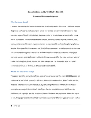
Results: The box plot of mean number of cases of cancer for 6 groups
boxplot(Rate.per.hundredthousand ~ Race, data=incidentcases_race, boxfill = "lightblue",
ylab="Rate per hundred thousand")

9. 9 | P a g e
Figure 1
The X and Y plot of different types of cancer and the % of surviving for 5 years.
xyplot(Percent.surviving.for.five.years ~ Site, data=cancer_type, col="red")
Figure 2

10. 10 | P a g e
The box plot of percent surviving for five years and cancer site
bwplot(Percent.surviving.for.five.years ~ Site, data=cancer_type)
Figure 3
The scatter plot of year of diagnosis and percent of both sexes surviving:
scatterplot(Percent.of.sex.surviving ~ Year.of.diagnosis, data = cancer_sex)

11. 11 | P a g e
Figure 4
Conclusion: On visualizing the plot (Figure 1) and looking at the results of ANOVA, the number
of cases for cancer is different among the various races and ethnic groups. The rate per
thousand is higher for the Black and low for the Asian/pacific islander and in between for
others. Hence it is statistically significant that the number of new cases for cancer is different
among various groups.
It is also evident that by visualizing the XYplot & Box plot (Figure 2 & 3) and the results
of ANOVA, the percent of surviving for five years is different among the various types of cancer.
From the study, it is evident that the survival rate for Lung and Bronchus cancer is very low
when compared to others and the survival rate for prostate and female breast cancers are
slightly higher than the others. Hence it is statistically significant that the percent surviving for 5
years is different among various types of cancer.
The paper also demonstrated the strong positive linear relationship between the year of
diagnosis of cancer and percent of surviving for 5 years for both sexes. When the years
increase, the 5 year survival rate increase linearly and provides a strong positive correlation of
0.99. The simple linear regression model is also derived by fitting a line to the scatter plot with
coefficients b0 = -1415, b1 = 0.74. Using the model we calculated the 5 year percent of survival
for the years 2015, 2016 and they are found to be 76.1% and 76.84%.