Ch 5 final seas factors

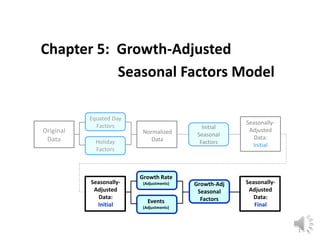
Chapter 5: Growth-Adjusted
1
Seasonal Factors Model
Original
Data
Equated Day
Factors
Holiday
Factors
Normalized
Data
Initial
Seasonal
Factors
Seasonally-
Adjusted
Data:
Initial
Seasonally-
Adjusted
Data:
Initial
Growth Rate
(Adjustments)
Events
(Adjustments)
Seasonally-
Adjusted
Data:
Final
Growth-Adj
Seasonal
Factors

Growth-Adjusted Seasonal Factors Model
2
This chapter will walk through the model structure that will be used to arrive
at the growth-adjusted seasonal factors.
1. Introduction
2. Inputs
3. Calc
4. Trend
1. Introduction – why growth-adjust?
2. Model Structure: Inputs
3. Model Structure: Calc
4. Model Structure: Trend
Introduction

Jan
Jan
Dec
Jan
Dec
Dec
Dec is much higher
than Jan each year
due to GROWTH,
not to seasonality.
XYZ Sales – with Growth
WITH
Growth
Year 1 Year 2 Year 3
3
Growth is removed so the seasonality measure only captures seasonality,
nothing else.
1. Introduction
2. Inputs
3. Calc
4. Trend

Jan
Dec
Dec is much higher
than Jan each year
due to GROWTH, not
to seasonality.
XYZ Sales – with & without Growth
WITH
Growth
WITHOUT
Growth
Without Growth,
the “true”
seasonal pattern is
more obvious.
Jan
Dec
4
Removing growth reveals the “true” relationship between January and
December (& all other months).
1. Introduction
2. Inputs
3. Calc
4. Trend

Sep
Seasonal pattern
can be further
skewed if Events
are included.
XYZ Sales – with & without Growth & Events
WITH
Growth
& Event
WITHOUT
Growth
&
Event
Adjusting for
Events as well as
Growth reveals
seasonal pattern.
New
product lifts
sales in Sep
by 15%
WITH
Growth
only
5
Adjustments need to be made for events as well.
1. Introduction
2. Inputs
3. Calc
4. Trend

6
After adjusting for growth & events, the “true” underlying seasonal pattern
emerges.
1. Introduction
2. Inputs
3. Calc
4. Trend
Seasonality:
Without Growth Adjustment
Seasonality:
With Growth Adjustment

7
The Excel model for developing the growth-adjusted seasonal factors, and for
estimating trend, has three parts.
1. Data Inputs (“Inputs” tab)
2. Calculations (“Calc” tab)
3. Trend Estimate (“Trend” tab)
1. Introduction
2. Inputs
3. Calc
4. Trend

8
The “Inputs” tab contains all the key information drawn from other files that
will be used to estimate trend.
1
2
9
10
11
12
13
14
15
16
17
18
19
20
21
22
23
24
197
198
199
200
201
202
203
204
249
250
251
279
A B C D E F
Key Inputs
Linked to diff file
Actuals
No. of
Days
Norm
Factor
Normalized
Data
Jan-01 27.844 21.7 1.05 26.510
Feb-01 21.631 19.1 0.92 23.459
Mar-01 27.970 22.0 1.07 26.229
Apr-01 25.529 19.7 0.95 26.799
May-01 24.568 21.9 1.06 23.175
Jun-01 24.674 21.0 1.02 24.284
Jul-01 23.878 19.8 0.96 24.883
Aug-01 23.591 22.8 1.10 21.354
Sep-01 25.417 15.0 0.72 35.098
Oct-01 30.229 22.6 1.09 27.692
Nov-01 26.672 20.4 0.99 27.054
Dec-01 25.506 17.8 0.86 29.529
Jan-02 29.943 21.3 1.03 29.056
Feb-02 26.255 19.1 0.92 28.474Jan-16 29.393 19.5 0.94 31.219Feb-16 29.857 20.0 0.97 30.918Mar-16 29.947 21.8 1.06 28.373Apr-16 26.183 21.0 1.02 25.739May-16 25.757 20.8 1.01 25.606Jun-16 30.123 22.0 1.06 28.334
Jul-16 22.328 19.9 0.96 23.217
Aug-16 23.490 23.0 1.11 21.141
Sep-16 25.282 20.8 1.01 25.100
Oct-16 22.795 20.5 0.99 22.964
Nov-16 22.000 20.4 0.99 22.307
Dec-16 22.000 19.0 0.92 23.878
Jan-17 0.000 20.4 0.99 0.000
Feb-17 0.000 19.0 0.92 0.000Jan-20 0.000 21.4 1.03 0.000Feb-20 0.000 19.0 0.92 0.000Mar-20 0.000 21.9 1.06 0.000Apr-20 0.000 20.8 1.01 0.000May-20 0.000 19.8 0.96 0.000Jun-20 0.000 21.9 1.06 0.000Jul-20 0.000 22.0 1.07 0.000Aug-20 0.000 20.9 1.01 0.000Sep-20 0.000 20.8 1.01 0.000Oct-20 0.000 21.6 1.05 0.000
Nov-20 0.000 19.3 0.93 0.000
Dec-20 0.000 19.3 0.94 0.000
Jan-21 0.000 0.0 0.00 0.000
TrendModel: Inputs
Update with
data thru Dec
2016
1. Introduction
2. Inputs
3. Calc
4. Trend
Model Structure: Inputs

9
The “Inputs” tab also brings in the seasonal factors – the initial factors already
developed, and the growth-adjusted factors to be developed in the model.
1
2
9
10
11
12
13
14
15
16
17
18
19
20
21
22
23
24
197
198
199
200
201
202
203
204
249
250
251
279
A B C D E F G H I J
Key Inputs
Linked to diff file
Actuals
No. of
Days
Norm
Factor
Normalized
Data None Initial
Growth-
Adjusted
Jan-01 27.844 21.7 1.05 26.510 1.00 1.00 1.03
Feb-01 21.631 19.1 0.92 23.459 1.00 0.96 0.98
Mar-01 27.970 22.0 1.07 26.229 1.00 1.00 1.01
Apr-01 25.529 19.7 0.95 26.799 1.00 0.99 1.01
May-01 24.568 21.9 1.06 23.175 1.00 0.99 1.00
Jun-01 24.674 21.0 1.02 24.284 1.00 1.02 1.03
Jul-01 23.878 19.8 0.96 24.883 1.00 0.98 0.97
Aug-01 23.591 22.8 1.10 21.354 1.00 0.93 0.89
Sep-01 25.417 15.0 0.72 35.098 1.00 1.00 1.01
Oct-01 30.229 22.6 1.09 27.692 1.00 1.02 1.02
Nov-01 26.672 20.4 0.99 27.054 1.00 1.03 1.00
Dec-01 25.506 17.8 0.86 29.529 1.00 1.07 1.06
Jan-02 29.943 21.3 1.03 29.056
Feb-02 26.255 19.1 0.92 28.474Jan-16 29.393 19.5 0.94 31.219Feb-16 29.857 20.0 0.97 30.918Mar-16 29.947 21.8 1.06 28.373Apr-16 26.183 21.0 1.02 25.739May-16 25.757 20.8 1.01 25.606Jun-16 30.123 22.0 1.06 28.334
Jul-16 22.328 19.9 0.96 23.217
Aug-16 23.490 23.0 1.11 21.141
Sep-16 25.282 20.8 1.01 25.100
Oct-16 22.795 20.5 0.99 22.964
Nov-16 22.000 20.4 0.99 22.307
Dec-16 22.000 19.0 0.92 23.878
Jan-17 0.000 20.4 0.99 0.000
Feb-17 0.000 19.0 0.92 0.000Jan-20 0.000 21.4 1.03 0.000Feb-20 0.000 19.0 0.92 0.000Mar-20 0.000 21.9 1.06 0.000Apr-20 0.000 20.8 1.01 0.000May-20 0.000 19.8 0.96 0.000Jun-20 0.000 21.9 1.06 0.000Jul-20 0.000 22.0 1.07 0.000Aug-20 0.000 20.9 1.01 0.000Sep-20 0.000 20.8 1.01 0.000Oct-20 0.000 21.6 1.05 0.000
Nov-20 0.000 19.3 0.93 0.000
Dec-20 0.000 19.3 0.94 0.000
Jan-21 0.000 0.0 0.00 0.000
Seasonal Factors
TrendModel: Inputs
Update with
data thru Dec
2016
1. Introduction
2. Inputs
3. Calc
4. Trend

10
The “Calc” tab is where all the calculations are performed. Except for
updating monthly data, this tab need never be touched.
TrendModel: Calc
1
2
7
8
9
10
11
12
13
14
15
16
17
18
19
20
21
22
23
197
198
199
200
201
202
203
204
205
A B C D E F G H I J K L M N O P Q R S T U
Calculations Unit: 1
In Use (1 = None; 2 = Initial; 3 = Final) : 2 Start: 25.000
Actuals
Adjust-
ments
Adjusted
Actuals
Normalization
Factors
Normalized
Data None Initial Revised In Use
Seasonally-
Adjusted:
Monthly
Seasonally-
Adjusted: 3-
Mo Avg
Growth
Rate
1-Time
Events
Estimated
Trend
Estimated
Trend
Values
Extrapolated
Trend
Extrapolated
Trend Values
(= Forecast)
Estimated (&
Forecast)
Trend
Actual (&
Forecast)
Values
Estimate vs
Actual: Diff
Jan-01 27.844 27.844 1.05 26.510 1.00 1.00 1.03 1.00 26.406 25.412 2.0% 0.0% 25.000 26.362 25.000 27.844 (2.844)
Feb-01 21.631 21.631 0.92 23.459 1.00 0.96 0.97 0.96 24.418 25.666 2.0% 0.0% 25.042 22.184 25.042 21.631 3.411
Mar-01 27.970 27.970 1.07 26.229 1.00 1.00 1.01 1.00 26.174 25.849 2.0% 0.0% 25.083 26.805 25.083 27.970 (2.887)
Apr-01 25.529 25.529 0.95 26.799 1.00 0.99 1.01 0.99 26.954 25.517 2.0% 0.0% 25.125 23.797 25.125 25.529 (0.404)
May-01 24.568 24.568 1.06 23.175 1.00 0.99 1.00 0.99 23.424 24.712 2.0% 0.0% 25.167 26.397 25.167 24.568 0.599
Jun-01 24.674 24.674 1.02 24.284 1.00 1.02 1.02 1.02 23.756 24.153 2.0% 0.0% 25.209 26.183 25.209 24.674 0.535
Jul-01 23.878 23.878 0.96 24.883 1.00 0.98 0.97 0.98 25.279 24.015 2.0% 0.0% 25.251 23.852 25.251 23.878 1.373
Aug-01 23.591 23.591 1.10 21.354 1.00 0.93 0.89 0.93 23.011 27.767 2.0% 0.0% 25.293 25.930 25.293 23.591 1.702
Sep-01 25.417 25.417 0.72 35.098 1.00 1.00 1.01 1.00 35.011 28.406 2.0% 30.0% 32.936 23.911 32.936 25.417 7.519
Oct-01 30.229 30.229 1.09 27.692 1.00 1.02 1.02 1.02 27.195 29.510 2.0% -20.0% 26.393 29.337 26.393 30.229 (3.836)
Nov-01 26.672 26.672 0.99 27.054 1.00 1.03 1.00 1.03 26.326 27.069 2.0% 0.0% 26.437 26.784 26.437 26.672 (0.235)
Dec-01 25.506 25.506 0.86 29.529 1.00 1.07 1.07 1.07 27.685 27.651 2.0% 0.0% 26.481 24.396 26.481 25.506 0.975
Jan-02 29.943 29.943 1.03 29.056 1.00 1.00 1.03 1.00 28.941 28.754 2.0% 0.0% 26.525 27.443 26.525 29.943 (3.418)Feb-02 26.255 26.255 0.92 28.474 1.00 0.96 0.97 0.96 29.637 28.775 2.0% 0.0% 26.569 23.537 26.569 26.255 0.314Mar-02 26.743 26.743 0.96 27.806 1.00 1.00 1.01 1.00 27.747 28.260 2.0% 0.0% 26.613 25.650 26.613 26.743 (0.130)Apr-02 28.761 28.761 1.06 27.239 1.00 0.99 1.01 0.99 27.397 27.017 2.0% 0.0% 26.658 27.985 26.658 28.761 (2.103)May-02 27.152 27.152 1.06 25.632 1.00 0.99 1.00 0.99 25.908 28.461 2.0% 0.0% 26.702 27.984 26.702 27.152 (0.450)Jun-02 31.740 31.740 0.97 32.791 1.00 1.02 1.02 1.02 32.079 33.049 2.0% 0.0% 26.747 26.464 26.747 31.740 (4.993)Jul-02 41.499 41.499 1.02 40.516 1.00 0.98 0.97 0.98 41.160 34.472 1.0% 0.0% 26.769 26.989 26.769 41.499 (14.730)Aug-02 29.511 29.511 1.05 28.003 1.00 0.93 0.89 0.93 30.177 33.477 1.0% 0.0% 26.791 26.200 26.791 29.511 (2.719)Sep-02 28.180 28.180 0.97 29.168 1.00 1.00 1.01 1.00 29.095 31.102 1.0% 0.0% 26.813 25.971 26.813 28.180 (1.367)Oct-02 38.061 38.061 1.10 34.657 1.00 1.02 1.02 1.02 34.034 31.178 1.0% 0.0% 26.836 30.011 26.836 38.061 (11.225)Nov-02 29.087 29.087 0.93 31.245 1.00 1.03 1.00 1.03 30.404 30.700 1.0% 0.0% 26.858 25.695 26.858 29.087 (2.229)Dec-02 26.205 26.205 0.89 29.503 1.00 1.07 1.07 1.07 27.660 29.293 1.0% 0.0% 26.881 25.466 26.881 26.205 0.676
Jul-16 22.328 22.328 0.96 23.217 1.00 0.98 0.97 0.98 23.585 24.695 1.0% 0.0% 30.790 29.149 30.790 22.328 6.821
Aug-16 23.490 23.490 1.11 21.141 1.00 0.93 0.89 0.93 22.782 23.801 1.0% 0.0% 30.815 31.773 30.815 23.490 8.283
Sep-16 25.282 25.282 1.01 25.100 1.00 1.00 1.01 1.00 25.037 23.457 1.0% 0.0% 30.841 31.143 30.841 25.282 5.861
Oct-16 22.795 22.795 0.99 22.964 1.00 1.02 1.02 1.02 22.552 24.850 1.0% 0.0% 30.867 31.200 30.867 22.795 8.405
Nov-16 27.327 27.327 0.99 27.708 1.00 1.03 1.00 1.03 26.963 24.306 1.0% 0.0% 30.892 31.310 30.892 27.327 3.983
Dec-16 23.000 23.000 0.92 24.963 1.00 1.07 1.07 1.07 23.404 25.183 1.0% 0.0% 30.918 30.385 30.918 23.000 7.385
Jan-17 0 0 0.99 0 1.00 1.00 1.03 1.00 1.0% 0.0% 30.944 30.666 30.944 30.666 0
Feb-17 0 0 0.92 0 1.00 0.96 0.97 0.96 1.0% 0.0% 30.970 27.396 30.970 27.396 0
Mar-17 0 0 1.12 0 1.00 1.00 1.01 1.00 1.0% 0.0% 30.996 34.673 30.996 34.673 0
E. Estimate & Actual
Seasonal Factors
A. Actual & Normalized Data B. Seasonally-Adjusted Data C. Estimated Trend D. Forecasts
1. Introduction
2. Inputs
3. Calc
4. Trend
Model Structure: Calc

11
The first part of the “Calc” brings in the original data, allows for adjustments if
needed, and calculates the normalized monthly amounts.
TrendModel: Calc
1
2
7
8
9
10
11
12
13
14
15
16
17
18
19
20
21
22
23
197
198
199
200
201
202
203
204
205
A B C D E F
In Use (1 = None; 2 = Initial; 3 = Final) :
Actuals
Adjust-
ments
Adjusted
Actuals
Normalization
Factors
Normalized
Data
Jan-01 27.844 27.844 1.05 26.510
Feb-01 21.631 21.631 0.92 23.459
Mar-01 27.970 27.970 1.07 26.229
Apr-01 25.529 25.529 0.95 26.799
May-01 24.568 24.568 1.06 23.175
Jun-01 24.674 24.674 1.02 24.284
Jul-01 23.878 23.878 0.96 24.883
Aug-01 23.591 23.591 1.10 21.354
Sep-01 25.417 25.417 0.72 35.098
Oct-01 30.229 30.229 1.09 27.692
Nov-01 26.672 26.672 0.99 27.054
Dec-01 25.506 25.506 0.86 29.529
Jan-02 29.943 29.943 1.03 29.056Feb-02 26.255 26.255 0.92 28.474Mar-02 26.743 26.743 0.96 27.806Apr-02 28.761 28.761 1.06 27.239May-02 27.152 27.152 1.06 25.632Jun-02 31.740 31.740 0.97 32.791Jul-02 41.499 41.499 1.02 40.516Aug-02 29.511 29.511 1.05 28.003Sep-02 28.180 28.180 0.97 29.168Oct-02 38.061 38.061 1.10 34.657Nov-02 29.087 29.087 0.93 31.245Dec-02 26.205 26.205 0.89 29.503
Jul-16 22.328 22.328 0.96 23.217
Aug-16 23.490 23.490 1.11 21.141
Sep-16 25.282 25.282 1.01 25.100
Oct-16 22.795 22.795 0.99 22.964
Nov-16 27.327 27.327 0.99 27.708
Dec-16 23.000 23.000 0.92 24.963
Jan-17 0 0 0.99 0
Feb-17 0 0 0.92 0
Mar-17 0 0 1.12 0
A. Actual & Normalized Data
1. Introduction
2. Inputs
3. Calc
4. Trend

12
The next section seasonally-adjusts the data, using one of the 3 sets of
seasonal factors.
TrendModel: Calc
1
2
7
8
9
10
11
12
13
14
15
16
17
18
19
20
21
22
23
197
198
199
200
201
202
203
204
205
A B C D E F G H I J K L
In Use (1 = None; 2 = Initial; 3 = Final) : 2
Actuals
Adjust-
ments
Adjusted
Actuals
Normalization
Factors
Normalized
Data None Initial Revised In Use
Seasonally-
Adjusted:
Monthly
Seasonally-
Adjusted: 3-
Mo Avg
Jan-01 27.844 27.844 1.05 26.510 1.00 1.00 1.03 1.00 26.406 25.412
Feb-01 21.631 21.631 0.92 23.459 1.00 0.96 0.97 0.96 24.418 25.666
Mar-01 27.970 27.970 1.07 26.229 1.00 1.00 1.01 1.00 26.174 25.849
Apr-01 25.529 25.529 0.95 26.799 1.00 0.99 1.01 0.99 26.954 25.517
May-01 24.568 24.568 1.06 23.175 1.00 0.99 1.00 0.99 23.424 24.712
Jun-01 24.674 24.674 1.02 24.284 1.00 1.02 1.02 1.02 23.756 24.153
Jul-01 23.878 23.878 0.96 24.883 1.00 0.98 0.97 0.98 25.279 24.015
Aug-01 23.591 23.591 1.10 21.354 1.00 0.93 0.89 0.93 23.011 27.767
Sep-01 25.417 25.417 0.72 35.098 1.00 1.00 1.01 1.00 35.011 28.406
Oct-01 30.229 30.229 1.09 27.692 1.00 1.02 1.02 1.02 27.195 29.510
Nov-01 26.672 26.672 0.99 27.054 1.00 1.03 1.00 1.03 26.326 27.069
Dec-01 25.506 25.506 0.86 29.529 1.00 1.07 1.07 1.07 27.685 27.651
Jan-02 29.943 29.943 1.03 29.056 1.00 1.00 1.03 1.00 28.941 28.754Feb-02 26.255 26.255 0.92 28.474 1.00 0.96 0.97 0.96 29.637 28.775Mar-02 26.743 26.743 0.96 27.806 1.00 1.00 1.01 1.00 27.747 28.260Apr-02 28.761 28.761 1.06 27.239 1.00 0.99 1.01 0.99 27.397 27.017May-02 27.152 27.152 1.06 25.632 1.00 0.99 1.00 0.99 25.908 28.461Jun-02 31.740 31.740 0.97 32.791 1.00 1.02 1.02 1.02 32.079 33.049Jul-02 41.499 41.499 1.02 40.516 1.00 0.98 0.97 0.98 41.160 34.472Aug-02 29.511 29.511 1.05 28.003 1.00 0.93 0.89 0.93 30.177 33.477Sep-02 28.180 28.180 0.97 29.168 1.00 1.00 1.01 1.00 29.095 31.102Oct-02 38.061 38.061 1.10 34.657 1.00 1.02 1.02 1.02 34.034 31.178Nov-02 29.087 29.087 0.93 31.245 1.00 1.03 1.00 1.03 30.404 30.700Dec-02 26.205 26.205 0.89 29.503 1.00 1.07 1.07 1.07 27.660 29.293
Jul-16 22.328 22.328 0.96 23.217 1.00 0.98 0.97 0.98 23.585 24.695
Aug-16 23.490 23.490 1.11 21.141 1.00 0.93 0.89 0.93 22.782 23.801
Sep-16 25.282 25.282 1.01 25.100 1.00 1.00 1.01 1.00 25.037 23.457
Oct-16 22.795 22.795 0.99 22.964 1.00 1.02 1.02 1.02 22.552 24.850
Nov-16 27.327 27.327 0.99 27.708 1.00 1.03 1.00 1.03 26.963 24.306
Dec-16 23.000 23.000 0.92 24.963 1.00 1.07 1.07 1.07 23.404 25.183
Jan-17 0 0 0.99 0 1.00 1.00 1.03 1.00
Feb-17 0 0 0.92 0 1.00 0.96 0.97 0.96
Mar-17 0 0 1.12 0 1.00 1.00 1.01 1.00
Seasonal Factors
A. Actual & Normalized Data B. Seasonally-Adjusted Data
1. Introduction
2. Inputs
3. Calc
4. Trend

13
The 3rd section estimates the data trend, using the Growth Rates and Events
that will be estimated in the “Trend” tab.
TrendModel: Calc
1
2
7
8
9
10
11
12
13
14
15
16
17
18
19
20
21
22
23
197
198
199
200
201
202
203
204
205
A E F G H I J K L M N O P
Calculations1
Normalization
Factors
Normalized
Data None Initial "Final" In Use
Seasonally-
Adjusted:
Monthly
Seasonally-
Adjusted: 3-
Mo Avg
Growth
Rate
1-Time
Events
Estimated
Trend
Estimated
Trend
Values
Jan-01 1.05 26.510 1.00 1.00 1.03 1.00 26.406 25.412 2.0% 0.0% 25.042 26.406
Feb-01 0.92 23.459 1.00 0.96 0.97 0.96 24.418 25.666 2.0% 0.0% 25.083 22.221
Mar-01 1.07 26.229 1.00 1.00 1.01 1.00 26.174 25.849 2.0% 0.0% 25.125 26.849
Apr-01 0.95 26.799 1.00 0.99 1.01 0.99 26.954 25.517 2.0% 0.0% 25.167 23.836
May-01 1.06 23.175 1.00 0.99 1.00 0.99 23.424 24.712 2.0% 0.0% 25.209 26.441
Jun-01 1.02 24.284 1.00 1.02 1.02 1.02 23.756 24.153 2.0% 0.0% 25.251 26.226
Jul-01 0.96 24.883 1.00 0.98 0.97 0.98 25.279 24.015 2.0% 0.0% 25.293 23.892
Aug-01 1.10 21.354 1.00 0.93 0.89 0.93 23.011 27.767 2.0% 0.0% 25.335 25.973
Sep-01 0.72 35.098 1.00 1.00 1.01 1.00 35.011 28.406 2.0% 30.0% 32.991 23.950
Oct-01 1.09 27.692 1.00 1.02 1.02 1.02 27.195 29.510 2.0% -20.0% 26.437 29.386
Nov-01 0.99 27.054 1.00 1.03 1.00 1.03 26.326 27.069 2.0% 0.0% 26.481 26.829
Dec-01 0.86 29.529 1.00 1.07 1.07 1.07 27.685 27.651 2.0% 0.0% 26.525 24.437
Jan-02 1.03 29.056 1.00 1.00 1.03 1.00 28.941 28.754 2.0% 0.0% 26.569 27.489Feb-02 0.92 28.474 1.00 0.96 0.97 0.96 29.637 28.775 2.0% 0.0% 26.613 23.576Mar-02 0.96 27.806 1.00 1.00 1.01 1.00 27.747 28.260 2.0% 0.0% 26.658 25.693Apr-02 1.06 27.239 1.00 0.99 1.01 0.99 27.397 27.017 2.0% 0.0% 26.702 28.032May-02 1.06 25.632 1.00 0.99 1.00 0.99 25.908 28.461 2.0% 0.0% 26.747 28.031Jun-02 0.97 32.791 1.00 1.02 1.02 1.02 32.079 33.049 2.0% 0.0% 26.791 26.508Jul-02 1.02 40.516 1.00 0.98 0.97 0.98 41.160 34.472 1.0% 0.0% 26.813 27.034Aug-02 1.05 28.003 1.00 0.93 0.89 0.93 30.177 33.477 1.0% 0.0% 26.836 26.244Sep-02 0.97 29.168 1.00 1.00 1.01 1.00 29.095 31.102 1.0% 0.0% 26.858 26.014Oct-02 1.10 34.657 1.00 1.02 1.02 1.02 34.034 31.178 1.0% 0.0% 26.881 30.061Nov-02 0.93 31.245 1.00 1.03 1.00 1.03 30.404 30.700 1.0% 0.0% 26.903 25.738Dec-02 0.89 29.503 1.00 1.07 1.07 1.07 27.660 29.293 1.0% 0.0% 26.925 25.509
Jul-16 0.96 23.217 1.00 0.98 0.97 0.98 23.585 24.695 1.0% 0.0% 30.841 29.197
Aug-16 1.11 21.141 1.00 0.93 0.89 0.93 22.782 23.801 1.0% 0.0% 30.867 31.826
Sep-16 1.01 25.100 1.00 1.00 1.01 1.00 25.037 23.457 1.0% 0.0% 30.892 31.195
Oct-16 0.99 22.964 1.00 1.02 1.02 1.02 22.552 24.850 0.0% 0.0% 30.892 31.226
Nov-16 0.99 27.708 1.00 1.03 1.00 1.03 26.963 24.306 0.0% 0.0% 30.892 31.310
Dec-16 0.92 24.963 1.00 1.07 1.07 1.07 23.404 25.183 0.0% 0.0% 30.892 30.359
Jan-17 0.99 0 1.00 1.00 1.03 1.00 0.0% 0.0%
Feb-17 0.92 0 1.00 0.96 0.97 0.96 0.0% 2.0%
Mar-17 1.12 0 1.00 1.00 1.01 1.00 0.0% 0.0%
Seasonal Factors
A. Actual & Normalized Data B. Seasonally-Adjusted Data C. Estimated Trend
1. Introduction
2. Inputs
3. Calc
4. Trend

14
The 4th section is the forecast, which takes the estimated trend and
extrapolates it using the assumptions for future growth rate & events.
TrendModel: Calc
1
2
7
8
9
10
11
12
13
14
15
16
17
18
19
20
21
22
23
197
198
199
200
201
202
203
204
205
A M N O P Q R
Calculations
Start: 25.000
Growth
Rate
1-Time
Events
Estimated
Trend
Estimated
Trend
Values
Extrapolated
Trend
Extrapolated
Trend Values
(= Forecast)
Jan-01 2.0% 0.0% 25.042 26.406
Feb-01 2.0% 0.0% 25.083 22.221
Mar-01 2.0% 0.0% 25.125 26.849
Apr-01 2.0% 0.0% 25.167 23.836
May-01 2.0% 0.0% 25.209 26.441
Jun-01 2.0% 0.0% 25.251 26.226
Jul-01 2.0% 0.0% 25.293 23.892
Aug-01 2.0% 0.0% 25.335 25.973
Sep-01 2.0% 30.0% 32.991 23.950
Oct-01 2.0% -20.0% 26.437 29.386
Nov-01 2.0% 0.0% 26.481 26.829
Dec-01 2.0% 0.0% 26.525 24.437
Jan-02 2.0% 0.0% 26.569 27.489Feb-02 2.0% 0.0% 26.613 23.576Mar-02 2.0% 0.0% 26.658 25.693Apr-02 2.0% 0.0% 26.702 28.032May-02 2.0% 0.0% 26.747 28.031Jun-02 2.0% 0.0% 26.791 26.508Jul-02 1.0% 0.0% 26.813 27.034Aug-02 1.0% 0.0% 26.836 26.244Sep-02 1.0% 0.0% 26.858 26.014Oct-02 1.0% 0.0% 26.881 30.061Nov-02 1.0% 0.0% 26.903 25.738Dec-02 1.0% 0.0% 26.925 25.509
Jul-16 1.0% 0.0% 30.841 29.197
Aug-16 1.0% 0.0% 30.867 31.826
Sep-16 1.0% 0.0% 30.892 31.195
Oct-16 0.0% 0.0% 30.892 31.226
Nov-16 0.0% 0.0% 30.892 31.310
Dec-16 0.0% 0.0% 30.892 30.359
Jan-17 0.0% 0.0% 30.892 30.614
Feb-17 0.0% 2.0% 31.510 27.874
Mar-17 0.0% 0.0% 31.510 35.249
C. Estimated Trend D. Forecasts
1. Introduction
2. Inputs
3. Calc
4. Trend

15
The 5th & final section picks up the past & projected trend, as well as the past
actuals and extrapolated trend values.
TrendModel: Calc
1
2
7
8
9
10
11
12
13
14
15
16
17
18
19
20
21
22
23
197
198
199
200
201
202
203
204
205
A B O P Q R S T U
Calculations
25.000
Actuals
Estimated
Trend
Estimated
Trend
Values
Extrapolated
Trend
Extrapolated
Trend Values
(= Forecast)
Estimated (&
Extrapolated)
Trend
Actual (&
Extrapolated)
Values
Estimate vs
Actual: Diff
Jan-01 27.844 25.042 26.406 25.042 27.844 (2.802)
Feb-01 21.631 25.083 22.221 25.083 21.631 3.452
Mar-01 27.970 25.125 26.849 25.125 27.970 (2.845)
Apr-01 25.529 25.167 23.836 25.167 25.529 (0.362)
May-01 24.568 25.209 26.441 25.209 24.568 0.641
Jun-01 24.674 25.251 26.226 25.251 24.674 0.577
Jul-01 23.878 25.293 23.892 25.293 23.878 1.415
Aug-01 23.591 25.335 25.973 25.335 23.591 1.745
Sep-01 25.417 32.991 23.950 32.991 25.417 7.574
Oct-01 30.229 26.437 29.386 26.437 30.229 (3.792)
Nov-01 26.672 26.481 26.829 26.481 26.672 (0.191)
Dec-01 25.506 26.525 24.437 26.525 25.506 1.019
Jan-02 29.943 26.569 27.489 26.569 29.943 (3.374)Feb-02 26.255 26.613 23.576 26.613 26.255 0.358Mar-02 26.743 26.658 25.693 26.658 26.743 (0.085)Apr-02 28.761 26.702 28.032 26.702 28.761 (2.059)May-02 27.152 26.747 28.031 26.747 27.152 (0.405)Jun-02 31.740 26.791 26.508 26.791 31.740 (4.948)Jul-02 41.499 26.813 27.034 26.813 41.499 (14.685)Aug-02 29.511 26.836 26.244 26.836 29.511 (2.675)Sep-02 28.180 26.858 26.014 26.858 28.180 (1.322)Oct-02 38.061 26.881 30.061 26.881 38.061 (11.180)Nov-02 29.087 26.903 25.738 26.903 29.087 (2.184)Dec-02 26.205 26.925 25.509 26.925 26.205 0.720
Jul-16 22.328 30.841 29.197 30.841 22.328 6.869
Aug-16 23.490 30.867 31.826 30.867 23.490 8.336
Sep-16 25.282 30.892 31.195 30.892 25.282 5.913
Oct-16 22.795 30.892 31.226 30.892 22.795 8.431
Nov-16 27.327 30.892 31.310 30.892 27.327 3.983
Dec-16 23.000 30.892 30.359 30.892 23.000 7.359
Jan-17 0 30.892 30.614 30.892 30.614 0
Feb-17 0 31.510 27.874 31.510 27.874 0
Mar-17 0 31.510 35.249 31.510 35.249 0
E. Estimate & ActualA. Actual & Normalized DataC. Estimated Trend D. Forecasts
1. Introduction
2. Inputs
3. Calc
4. Trend
Revise Col. U & its explanation.
Change next page and start page
showing this as well

16
The bottom of the “Calc” tab calculates annual totals for all the columns.
TrendModel: Calc
1
2
7
8
9
10
299
300
301
302
303
304
305
306
307
308
309
310
311
312
313
314
315
316
317
318
319
320
A B C D E F G H I J K L M N O P Q R S T U
Actuals
Adjust-
ments
Adjusted
Actuals
Normalization
Factors
Normalized
Data None Initial "Final" In Use
Seasonally-
Adjusted:
Monthly
Seasonally-
Adjusted: 3-
Mo Avg
Growth
Rate
1-Time
Events
Estimated
Trend
Estimated
Trend
Values
Extrapolated
Trend
Extrapolated
Trend Values
(= Forecast)
Estimated (&
Extrapolated)
Trend
Actual (&
Extrapolated)
Values
Estimate vs
Actual: Diff
Annual Totals
2001 308 0 308 0.983 316 1.000 1.000 1.000 1.000 316 316 2.0% 10.0% 314 306 0 0 314 308 6
2002 363 0 363 0.997 364 1.000 1.000 1.000 1.000 364 365 1.5% 0.0% 321 320 0 0 321 363 (42)
2003 352 0 352 1.000 352 1.000 1.000 1.000 1.000 352 353 1.0% 0.0% 325 325 0 0 325 352 (28)
2004 370 0 370 1.003 370 1.000 1.000 1.000 1.000 369 367 1.0% 0.0% 328 329 0 0 328 370 (42)
2005 415 0 415 1.004 414 1.000 1.000 1.000 1.000 414 416 1.0% 0.0% 331 332 0 0 331 415 (84)
2006 458 0 458 0.997 460 1.000 1.000 1.000 1.000 460 459 1.0% 0.0% 335 334 0 0 335 458 (124)
2007 532 0 532 0.999 531 1.000 1.000 1.000 1.000 533 537 1.0% 0.0% 338 338 0 0 338 532 (194)
2008 660 0 660 1.003 656 1.000 1.000 1.000 1.000 656 650 1.0% 0.0% 342 343 0 0 342 660 (319)
2009 549 0 549 0.999 550 1.000 1.000 1.000 1.000 551 551 1.0% 0.0% 345 344 0 0 345 549 (204)
2010 445 0 445 0.999 445 1.000 1.000 1.000 1.000 446 447 1.0% 0.0% 348 348 0 0 348 445 (96)
2011 384 0 384 1.003 381 1.000 1.000 1.000 1.000 382 381 1.0% 0.0% 352 353 0 0 352 384 (32)
2012 287 0 287 0.998 288 1.000 1.000 1.000 1.000 288 288 1.0% 0.0% 355 354 0 0 355 287 69
2013 261 0 261 0.996 262 1.000 1.000 1.000 1.000 262 262 1.0% 0.0% 359 357 0 0 359 261 98
2014 262 0 262 1.000 262 1.000 1.000 1.000 1.000 262 261 1.0% 0.0% 363 362 0 0 363 262 101
2015 299 0 299 0.999 300 1.000 1.000 1.000 1.000 300 301 1.0% 0.0% 366 366 0 0 366 299 67
2016 315 0 315 1.002 315 1.000 1.000 1.000 1.000 315 315 0.8% 0.0% 370 370 0 0 370 315 55
2017 0 0 0 0.997 0 1.000 1.000 1.000 1.000 0 0 0.0% 2.0% 0 0 378 376 378 376 0
2018 0 0 0 0.999 0 1.000 1.000 1.000 1.000 0 0 0.0% 0.0% 0 0 378 377 378 377 0
2019 0 0 0 0.996 0 1.000 1.000 1.000 1.000 0 0 0.0% 0.0% 0 0 378 376 378 376 0
2020 0 0 0 1.004 0 1.000 1.000 1.000 1.000 0 0 0.0% 0.0% 0 0 378 379 378 379 0
E. Estimate & Actual
Seasonal Factors
A. Actual & Normalized Data B. Seasonally-Adjusted Data C. Estimated Trend D. Forecasts
1. Introduction
2. Inputs
3. Calc
4. Trend

17
The “Trend” tab is divided into
three sections.
TrendModel: Trend
1
8
9
10
11
12
13
14
15
16
17
18
19
20
21
22
23
24
25
26
29
30
31
32
33
34
35
36
37
38
39
40
41
42
43
49
50
51
52
53
54
55
56
57
58
59
60
61
62
97
98
99
100
101
102
103
104
105
106
107
108
109
110
111
112
113
114
119
120
121
122
123
124
125
126
127
128
129
130
131
132
133
134
139
140
141
142
143
144
145
146
147
148
149
150
151
152
153
154
155
159
160
161
162
163
164
165
166
167
168
169
170
171
172
173
174
175
179
180
181
182
183
184
185
186
187
188
189
190
191
192
193
194
195
196
199
200
201
202
203
204
205
206
207
208
209
210
211
212
213
214
215
219
220
221
222
223
224
225
226
227
228
229
230
231
232
233
234
235
236
A C D E F G H I J K L M N O P Q R S X Y Z AA AB AC AD AE AF AG AH AI AJ
Estimating Trend Seasonal Factors In Use: Initial 2
(1 = None; 2 = Initial; 3 = Final)
Growth Rate
2001 2002 2003 2004 2005 2006 2007 2008 2009 2010 2011 2012 2013 2014 2015 2016 2017
Jan 2.0% 2.0% 1.0% 1.0% 1.0% 1.0% 1.0% 1.0% 1.0% 1.0% 1.0% 1.0% 1.0% 1.0% 1.0% 1.0% 0.0%
Feb 2.0% 2.0% 1.0% 1.0% 1.0% 1.0% 1.0% 1.0% 1.0% 1.0% 1.0% 1.0% 1.0% 1.0% 1.0% 1.0% 0.0%
Mar 2.0% 2.0% 1.0% 1.0% 1.0% 1.0% 1.0% 1.0% 1.0% 1.0% 1.0% 1.0% 1.0% 1.0% 1.0% 1.0% 0.0%
Apr 2.0% 2.0% 1.0% 1.0% 1.0% 1.0% 1.0% 1.0% 1.0% 1.0% 1.0% 1.0% 1.0% 1.0% 1.0% 1.0% 0.0%
May 2.0% 2.0% 1.0% 1.0% 1.0% 1.0% 1.0% 1.0% 1.0% 1.0% 1.0% 1.0% 1.0% 1.0% 1.0% 1.0% 0.0%
Jun 2.0% 2.0% 1.0% 1.0% 1.0% 1.0% 1.0% 1.0% 1.0% 1.0% 1.0% 1.0% 1.0% 1.0% 1.0% 1.0% 0.0%
Jul 2.0% 1.0% 1.0% 1.0% 1.0% 1.0% 1.0% 1.0% 1.0% 1.0% 1.0% 1.0% 1.0% 1.0% 1.0% 1.0% 0.0%
Aug 2.0% 1.0% 1.0% 1.0% 1.0% 1.0% 1.0% 1.0% 1.0% 1.0% 1.0% 1.0% 1.0% 1.0% 1.0% 1.0% 0.0%
Sep 2.0% 1.0% 1.0% 1.0% 1.0% 1.0% 1.0% 1.0% 1.0% 1.0% 1.0% 1.0% 1.0% 1.0% 1.0% 1.0% 0.0%
Oct 2.0% 1.0% 1.0% 1.0% 1.0% 1.0% 1.0% 1.0% 1.0% 1.0% 1.0% 1.0% 1.0% 1.0% 1.0% 0.0% 0.0%
Nov 2.0% 1.0% 1.0% 1.0% 1.0% 1.0% 1.0% 1.0% 1.0% 1.0% 1.0% 1.0% 1.0% 1.0% 1.0% 0.0% 0.0%
Dec 2.0% 1.0% 1.0% 1.0% 1.0% 1.0% 1.0% 1.0% 1.0% 1.0% 1.0% 1.0% 1.0% 1.0% 1.0% 0.0% 0.0%
Start
25.0
Events
2001 2002 2003 2004 2005 2006 2007 2008 2009 2010 2011 2012 2013 2014 2015 2016 2017
Jan
Feb 2.0%
Mar
Apr
May
Jun
Jul
Aug
Sep 30.0%
Oct -20.0%
Nov
Dec
Actuals vs Estimate by Year
2001 2002 2003 2004 2005 2006 2007 2008 2009 2010 2011 2012 2013 2014 2015 2016 2017
Actual 307.5 363.1 352.4 369.6 415.1 458.5 532.0 660.3 549.3 444.7 383.9 286.8 260.7 261.9 299.1 315.5 0.0
Est 306.4 319.9 324.8 329.0 332.4 333.5 337.5 342.5 344.5 348.1 352.7 354.4 357.3 362.4 365.8 370.4 376.1
Diff -1.1 -43.2 -27.6 -40.6 -82.7 -125.0 -194.5 -317.8 -204.8 -96.6 -31.2 67.6 96.7 100.5 66.7 54.9
% Diff -0.3% -11.9% -7.8% -11.0% -19.9% -27.3% -36.6% -48.1% -37.3% -21.7% -8.1% 23.6% 37.1% 38.4% 22.3% 17.4%
Total
2001-16 YTD
Actual 6,260 315.5
Est 5,482 370.4
Diff (779) 54.9
% Diff -12.4% 17.4%
Seasonal Factors
Normalized Data
2001 2002 2003 2004 2005 2006 2007 2008 2009 2010 2011 2012 2013 2014 2015 2016 2017
Jan 26.5 29.1 29.9 34.2 33.2 39.6 38.3 58.1 46.4 35.6 33.2 24.7 22.0 20.7 24.5 31.2 0.0
Feb 23.5 28.5 27.5 30.6 33.0 37.5 40.0 47.0 54.6 35.5 31.8 24.4 22.2 22.1 23.2 30.9 0.0
Mar 26.2 27.8 29.9 30.7 35.6 35.9 43.9 55.7 61.8 33.2 31.9 24.8 22.4 22.1 24.1 28.4 0.0
Apr 26.8 27.2 29.6 31.9 35.8 37.2 40.2 43.9 53.5 41.0 27.8 24.6 22.2 21.8 22.6 25.7 0.0
May 23.2 25.6 31.0 31.5 32.2 41.5 41.3 42.5 52.6 54.4 28.5 26.4 21.9 19.4 21.8 25.6 0.0
Jun 24.3 32.8 31.5 27.1 32.1 41.4 45.0 50.5 43.7 43.5 30.0 26.4 26.0 21.1 24.6 28.3 0.0
Jul 24.9 40.5 30.2 29.3 31.5 38.7 49.0 60.5 38.4 36.5 27.3 24.5 20.5 19.2 23.0 23.2 0.0
Aug 21.4 28.0 25.1 25.9 30.6 33.3 55.4 44.6 41.2 32.0 43.6 20.2 19.1 17.8 27.5 21.1 0.0
Sep 35.1 29.2 29.7 27.7 36.1 37.3 40.3 70.1 42.8 32.2 35.0 23.9 21.8 21.4 27.8 25.1 0.0
Oct 27.7 34.7 30.0 32.9 40.7 39.1 41.6 75.7 41.4 33.9 34.5 20.2 20.8 26.7 26.4 23.0 0.0
Nov 27.1 31.2 27.8 32.4 36.4 40.4 52.2 57.3 35.2 33.9 29.6 23.1 20.3 22.4 25.2 27.7 0.0
Dec 29.5 29.5 29.6 35.2 36.8 38.2 44.1 50.2 38.1 33.7 27.6 24.7 23.0 27.6 28.9 25.0 0.0
Growth Rate (Monthly Basis)
2001 2002 2003 2004 2005 2006 2007 2008 2009 2010 2011 2012 2013 2014 2015 2016 2017
Jan 0.2% 0.2% 0.1% 0.1% 0.1% 0.1% 0.1% 0.1% 0.1% 0.1% 0.1% 0.1% 0.1% 0.1% 0.1% 0.1% 0.0%
Feb 0.2% 0.2% 0.1% 0.1% 0.1% 0.1% 0.1% 0.1% 0.1% 0.1% 0.1% 0.1% 0.1% 0.1% 0.1% 0.1% 2.0%
Mar 0.2% 0.2% 0.1% 0.1% 0.1% 0.1% 0.1% 0.1% 0.1% 0.1% 0.1% 0.1% 0.1% 0.1% 0.1% 0.1% 0.0%
Apr 0.2% 0.2% 0.1% 0.1% 0.1% 0.1% 0.1% 0.1% 0.1% 0.1% 0.1% 0.1% 0.1% 0.1% 0.1% 0.1% 0.0%
May 0.2% 0.2% 0.1% 0.1% 0.1% 0.1% 0.1% 0.1% 0.1% 0.1% 0.1% 0.1% 0.1% 0.1% 0.1% 0.1% 0.0%
Jun 0.2% 0.2% 0.1% 0.1% 0.1% 0.1% 0.1% 0.1% 0.1% 0.1% 0.1% 0.1% 0.1% 0.1% 0.1% 0.1% 0.0%
Jul 0.2% 0.1% 0.1% 0.1% 0.1% 0.1% 0.1% 0.1% 0.1% 0.1% 0.1% 0.1% 0.1% 0.1% 0.1% 0.1% 0.0%
Aug 0.2% 0.1% 0.1% 0.1% 0.1% 0.1% 0.1% 0.1% 0.1% 0.1% 0.1% 0.1% 0.1% 0.1% 0.1% 0.1% 0.0%
Sep 30.2% 0.1% 0.1% 0.1% 0.1% 0.1% 0.1% 0.1% 0.1% 0.1% 0.1% 0.1% 0.1% 0.1% 0.1% 0.1% 0.0%
Oct -19.9% 0.1% 0.1% 0.1% 0.1% 0.1% 0.1% 0.1% 0.1% 0.1% 0.1% 0.1% 0.1% 0.1% 0.1% 0.0% 0.0%
Nov 0.2% 0.1% 0.1% 0.1% 0.1% 0.1% 0.1% 0.1% 0.1% 0.1% 0.1% 0.1% 0.1% 0.1% 0.1% 0.0% 0.0%
Dec 0.2% 0.1% 0.1% 0.1% 0.1% 0.1% 0.1% 0.1% 0.1% 0.1% 0.1% 0.1% 0.1% 0.1% 0.1% 0.0% 0.0%
Cumulative Growth Rate
2001 2002 2003 2004 2005 2006 2007 2008 2009 2010 2011 2012 2013 2014 2015 2016 2017
Jan 0.2% 0.2% 0.1% 0.1% 0.1% 0.1% 0.1% 0.1% 0.1% 0.1% 0.1% 0.1% 0.1% 0.1% 0.1% 0.1% 0.0%
Feb 0.3% 0.3% 0.2% 0.2% 0.2% 0.2% 0.2% 0.2% 0.2% 0.2% 0.2% 0.2% 0.2% 0.2% 0.2% 0.2% 2.0%
Mar 0.5% 0.5% 0.3% 0.3% 0.3% 0.3% 0.3% 0.3% 0.3% 0.3% 0.3% 0.3% 0.3% 0.3% 0.3% 0.3% 2.0%
Apr 0.7% 0.7% 0.3% 0.3% 0.3% 0.3% 0.3% 0.3% 0.3% 0.3% 0.3% 0.3% 0.3% 0.3% 0.3% 0.3% 2.0%
May 0.8% 0.8% 0.4% 0.4% 0.4% 0.4% 0.4% 0.4% 0.4% 0.4% 0.4% 0.4% 0.4% 0.4% 0.4% 0.4% 2.0%
Jun 1.0% 1.0% 0.5% 0.5% 0.5% 0.5% 0.5% 0.5% 0.5% 0.5% 0.5% 0.5% 0.5% 0.5% 0.5% 0.5% 2.0%
Jul 1.2% 1.1% 0.6% 0.6% 0.6% 0.6% 0.6% 0.6% 0.6% 0.6% 0.6% 0.6% 0.6% 0.6% 0.6% 0.6% 2.0%
Aug 1.3% 1.2% 0.7% 0.7% 0.7% 0.7% 0.7% 0.7% 0.7% 0.7% 0.7% 0.7% 0.7% 0.7% 0.7% 0.7% 2.0%
Sep 32.0% 1.3% 0.8% 0.8% 0.8% 0.8% 0.8% 0.8% 0.8% 0.8% 0.8% 0.8% 0.8% 0.8% 0.8% 0.8% 2.0%
Oct 5.7% 1.3% 0.8% 0.8% 0.8% 0.8% 0.8% 0.8% 0.8% 0.8% 0.8% 0.8% 0.8% 0.8% 0.8% 0.8% 2.0%
Nov 5.9% 1.4% 0.9% 0.9% 0.9% 0.9% 0.9% 0.9% 0.9% 0.9% 0.9% 0.9% 0.9% 0.9% 0.9% 0.8% 2.0%
Dec 6.1% 1.5% 1.0% 1.0% 1.0% 1.0% 1.0% 1.0% 1.0% 1.0% 1.0% 1.0% 1.0% 1.0% 1.0% 0.8% 2.0%
Avg 4.6% 0.9% 0.5% 0.5% 0.5% 0.5% 0.5% 0.5% 0.5% 0.5% 0.5% 0.5% 0.5% 0.5% 0.5% 0.5% 1.8%
Indexed Cumulative Growth
2001 2002 2003 2004 2005 2006 2007 2008 2009 2010 2011 2012 2013 2014 2015 2016 2017
Jan 0.96 0.99 1.00 1.00 1.00 1.00 1.00 1.00 1.00 1.00 1.00 1.00 1.00 1.00 1.00 1.00 0.98
Feb 0.96 0.99 1.00 1.00 1.00 1.00 1.00 1.00 1.00 1.00 1.00 1.00 1.00 1.00 1.00 1.00 1.00
Mar 0.96 1.00 1.00 1.00 1.00 1.00 1.00 1.00 1.00 1.00 1.00 1.00 1.00 1.00 1.00 1.00 1.00
Apr 0.96 1.00 1.00 1.00 1.00 1.00 1.00 1.00 1.00 1.00 1.00 1.00 1.00 1.00 1.00 1.00 1.00
May 0.96 1.00 1.00 1.00 1.00 1.00 1.00 1.00 1.00 1.00 1.00 1.00 1.00 1.00 1.00 1.00 1.00
Jun 0.97 1.00 1.00 1.00 1.00 1.00 1.00 1.00 1.00 1.00 1.00 1.00 1.00 1.00 1.00 1.00 1.00
Jul 0.97 1.00 1.00 1.00 1.00 1.00 1.00 1.00 1.00 1.00 1.00 1.00 1.00 1.00 1.00 1.00 1.00
Aug 0.97 1.00 1.00 1.00 1.00 1.00 1.00 1.00 1.00 1.00 1.00 1.00 1.00 1.00 1.00 1.00 1.00
Sep 1.26 1.00 1.00 1.00 1.00 1.00 1.00 1.00 1.00 1.00 1.00 1.00 1.00 1.00 1.00 1.00 1.00
Oct 1.01 1.00 1.00 1.00 1.00 1.00 1.00 1.00 1.00 1.00 1.00 1.00 1.00 1.00 1.00 1.00 1.00
Nov 1.01 1.00 1.00 1.00 1.00 1.00 1.00 1.00 1.00 1.00 1.00 1.00 1.00 1.00 1.00 1.00 1.00
Dec 1.01 1.01 1.00 1.00 1.00 1.00 1.00 1.00 1.00 1.00 1.00 1.00 1.00 1.00 1.00 1.00 1.00
Avg 1.000 1.000 1.000 1.000 1.000 1.000 1.000 1.000 1.000 1.000 1.000 1.000 1.000 1.000 1.000 1.000 1.000
Growth-Adjusted Normalized Data
2001 2002 2003 2004 2005 2006 2007 2008 2009 2010 2011 2012 2013 2014 2015 2016 2017
Jan 27.7 29.3 30.1 34.3 33.3 39.8 38.5 58.3 46.7 35.8 33.3 24.8 22.1 20.8 24.6 31.3 0.0
Feb 24.5 28.6 27.6 30.7 33.1 37.6 40.1 47.2 54.8 35.6 31.9 24.5 22.3 22.2 23.3 31.0 0.0
Mar 27.3 27.9 30.0 30.8 35.7 36.0 44.0 55.9 61.9 33.3 32.0 24.9 22.4 22.1 24.2 28.4 0.0
Apr 27.9 27.3 29.7 32.0 35.9 37.2 40.3 44.0 53.6 41.1 27.9 24.6 22.2 21.8 22.6 25.8 0.0
May 24.1 25.7 31.0 31.5 32.2 41.5 41.4 42.6 52.6 54.5 28.6 26.4 21.9 19.4 21.9 25.6 0.0
Jun 25.2 32.8 31.5 27.2 32.1 41.5 45.1 50.6 43.7 43.6 30.0 26.4 26.0 21.1 24.6 28.3 0.0
Jul 25.7 40.5 30.2 29.3 31.5 38.6 49.0 60.4 38.4 36.5 27.2 24.5 20.5 19.2 23.0 23.2 0.0
Aug 22.1 27.9 25.1 25.9 30.6 33.2 55.4 44.6 41.1 32.0 43.6 20.2 19.0 17.8 27.4 21.1 0.0
Sep 27.8 29.1 29.7 27.6 36.0 37.2 40.2 70.0 42.7 32.1 34.9 23.9 21.7 21.3 27.8 25.0 0.0
Oct 27.4 34.5 29.9 32.8 40.6 39.0 41.5 75.5 41.2 33.8 34.4 20.2 20.7 26.6 26.4 22.9 0.0
Nov 26.7 31.1 27.7 32.3 36.3 40.3 52.0 57.1 35.0 33.7 29.5 23.0 20.3 22.3 25.1 27.6 0.0
Dec 29.1 29.3 29.5 35.0 36.7 38.0 43.9 50.0 37.9 33.6 27.5 24.6 22.9 27.5 28.7 24.9 0.0
Avg 26.3 30.3 29.3 30.8 34.5 38.3 44.3 54.7 45.8 37.1 31.7 24.0 21.8 21.8 25.0 26.3 0.0
0.2% 0.0% 0.0% 0.0% 0.0% 0.0% 0.0% 0.0% 0.0% 0.0% 0.0% 0.0% 0.0% 0.0% 0.0% 0.0%
Growth-Adjusted Normalized Data: Factored Max Permitted Standard Deviations: 2.0
2001 2002 2003 2004 2005 2006 2007 2008 2009 2010 2011 2012 2013 2014 2015 2016 2017 Avg Std Dev Low High Wtd Avg
Jan 1.05 0.97 1.03 1.11 0.97 1.04 0.87 1.07 1.02 0.96 1.05 1.03 1.01 0.95 0.98 1.19 1.02 0.07 0.87 1.17 1.03
Feb 0.93 0.94 0.94 1.00 0.96 0.98 0.91 0.86 1.20 0.96 1.01 1.02 1.02 1.02 0.93 1.18 0.99 0.09 0.81 1.17 0.97
Mar 1.04 0.92 1.02 1.00 1.03 0.94 0.99 1.02 1.35 0.90 1.01 1.04 1.03 1.01 0.97 1.08 1.02 0.10 0.82 1.22 1.01
Apr 1.06 0.90 1.01 1.04 1.04 0.97 0.91 0.81 1.17 1.11 0.88 1.03 1.02 1.00 0.91 0.98 0.99 0.09 0.80 1.17 1.01
May 0.91 0.85 1.06 1.02 0.93 1.08 0.93 0.78 1.15 1.47 0.90 1.10 1.00 0.89 0.88 0.98 1.00 0.16 0.67 1.32 1.00
Jun 0.96 1.08 1.07 0.88 0.93 1.08 1.02 0.92 0.95 1.17 0.95 1.10 1.19 0.97 0.99 1.08 1.02 0.09 0.84 1.20 1.02
Jul 0.98 1.33 1.03 0.95 0.91 1.01 1.11 1.11 0.84 0.98 0.86 1.02 0.94 0.88 0.92 0.88 0.98 0.12 0.74 1.23 0.97
Aug 0.84 0.92 0.86 0.84 0.89 0.87 1.25 0.82 0.90 0.86 1.37 0.84 0.87 0.81 1.10 0.80 0.93 0.17 0.59 1.26 0.89
Sep 1.06 0.96 1.01 0.90 1.04 0.97 0.91 1.28 0.93 0.87 1.10 0.99 0.99 0.98 1.11 0.95 1.00 0.10 0.80 1.21 1.01
Oct 1.04 1.14 1.02 1.07 1.18 1.02 0.94 1.38 0.90 0.91 1.08 0.84 0.95 1.22 1.06 0.87 1.04 0.14 0.75 1.32 1.02
Nov 1.02 1.03 0.95 1.05 1.05 1.05 1.17 1.04 0.76 0.91 0.93 0.96 0.93 1.02 1.01 1.05 1.00 0.09 0.81 1.18 1.00
Dec 1.11 0.97 1.00 1.14 1.06 0.99 0.99 0.91 0.83 0.90 0.87 1.02 1.05 1.26 1.15 0.95 1.01 0.11 0.79 1.24 1.07
Avg 1.00 1.00 1.00 1.00 1.00 1.00 1.00 1.00 1.00 1.00 1.00 1.00 1.00 1.00 1.00 1.00 1.00 0.11 0.78 1.22 1.00
Data Accepted?
2001 2002 2003 2004 2005 2006 2007 2008 2009 2010 2011 2012 2013 2014 2015 2016 2017 Total
Jan 1 1 1 1 1 1 0 1 1 1 1 1 1 1 1 0
Feb 1 1 1 1 1 1 1 1 0 1 1 1 1 1 1 0
Mar 1 1 1 1 1 1 1 1 0 1 1 1 1 1 1 1
Apr 1 1 1 1 1 1 1 1 1 1 1 1 1 1 1 1
May 1 1 1 1 1 1 1 1 1 0 1 1 1 1 1 1
Jun 1 1 1 1 1 1 1 1 1 1 1 1 1 1 1 1
Jul 1 0 1 1 1 1 1 1 1 1 1 1 1 1 1 1
Aug 1 1 1 1 1 1 1 1 1 1 0 1 1 1 1 1
Sep 1 1 1 1 1 1 1 0 1 1 1 1 1 1 1 1
Oct 1 1 1 1 1 1 1 0 1 1 1 1 1 1 1 1
Nov 1 1 1 1 1 1 1 1 0 1 1 1 1 1 1 1
Dec 1 1 1 1 1 1 1 1 1 1 1 1 1 0 1 1
OK? 1 0 1 1 1 1 0 0 0 0 0 1 1 0 1 0 8
Use Std
Dev? 1 1 1 1 1 1 1 1 1 1 1 1 1 1 1 1 1
Seasonal
Factor
Weights
1 0 1 1 1 1 0 0 0 0 0 1 1 0 1 0 0 8
Accepted Range
022.0
24.0
26.0
28.0
30.0
32.0
34.0
36.0
38.0
40.0
Jan-01 Jan-02 Jan-03 Jan-04
Sales
Volumes
(Billions)
NYSE Monthly Sales Volumes
Seasonally-Adjusted
Actual (& Extrapolated) Values
Seasonally-Adjusted: Monthly
Seasonally-Adjusted: 3-Mo Avg
0.70
0.80
0.90
1.00
1.10
1.20
1.30
Jan Feb Mar Apr May Jun Jul Aug Sep Oct Nov Dec
Seasonal Factors Final
Initial
Low
High
Trend
Estimates
Seasonal
Factors
Calculation
Chart
1. Introduction
2. Inputs
3. Calc
4. Trend
Model Structure: Trend

1
8
9
10
11
12
13
14
15
16
17
18
19
20
21
22
23
24
25
26
29
30
31
32
33
34
35
36
37
38
39
40
41
42
43
49
50
51
52
53
54
55
56
57
58
59
60
61
62
A C D E F G H I J K L M N O P Q R S X
Estimating Trend
Growth Rate
2001 2002 2003 2004 2005 2006 2007 2008 2009 2010 2011 2012 2013 2014 2015 2016 2017
Jan 2.0% 2.0% 1.0% 1.0% 1.0% 1.0% 1.0% 1.0% 1.0% 1.0% 1.0% 1.0% 1.0% 1.0% 1.0% 1.0% 0.0%
Feb 2.0% 2.0% 1.0% 1.0% 1.0% 1.0% 1.0% 1.0% 1.0% 1.0% 1.0% 1.0% 1.0% 1.0% 1.0% 1.0% 0.0%
Mar 2.0% 2.0% 1.0% 1.0% 1.0% 1.0% 1.0% 1.0% 1.0% 1.0% 1.0% 1.0% 1.0% 1.0% 1.0% 1.0% 0.0%
Apr 2.0% 2.0% 1.0% 1.0% 1.0% 1.0% 1.0% 1.0% 1.0% 1.0% 1.0% 1.0% 1.0% 1.0% 1.0% 1.0% 0.0%
May 2.0% 2.0% 1.0% 1.0% 1.0% 1.0% 1.0% 1.0% 1.0% 1.0% 1.0% 1.0% 1.0% 1.0% 1.0% 1.0% 0.0%
Jun 2.0% 2.0% 1.0% 1.0% 1.0% 1.0% 1.0% 1.0% 1.0% 1.0% 1.0% 1.0% 1.0% 1.0% 1.0% 1.0% 0.0%
Jul 2.0% 1.0% 1.0% 1.0% 1.0% 1.0% 1.0% 1.0% 1.0% 1.0% 1.0% 1.0% 1.0% 1.0% 1.0% 1.0% 0.0%
Aug 2.0% 1.0% 1.0% 1.0% 1.0% 1.0% 1.0% 1.0% 1.0% 1.0% 1.0% 1.0% 1.0% 1.0% 1.0% 1.0% 0.0%
Sep 2.0% 1.0% 1.0% 1.0% 1.0% 1.0% 1.0% 1.0% 1.0% 1.0% 1.0% 1.0% 1.0% 1.0% 1.0% 1.0% 0.0%
Oct 2.0% 1.0% 1.0% 1.0% 1.0% 1.0% 1.0% 1.0% 1.0% 1.0% 1.0% 1.0% 1.0% 1.0% 1.0% 0.0% 0.0%
Nov 2.0% 1.0% 1.0% 1.0% 1.0% 1.0% 1.0% 1.0% 1.0% 1.0% 1.0% 1.0% 1.0% 1.0% 1.0% 0.0% 0.0%
Dec 2.0% 1.0% 1.0% 1.0% 1.0% 1.0% 1.0% 1.0% 1.0% 1.0% 1.0% 1.0% 1.0% 1.0% 1.0% 0.0% 0.0%
Start
25.0
Events
2001 2002 2003 2004 2005 2006 2007 2008 2009 2010 2011 2012 2013 2014 2015 2016 2017
Jan
Feb 2.0%
Mar
Apr
May
Jun
Jul 10.0%
Aug
Sep 30.0%
Oct -20.0%
Nov
Dec
2001 2002 2003 2004 2005 2006 2007 2008 2009 2010 2011 2012 2013 2014 2015 2016 2017
Actual 307.5 363.1 352.4 369.6 415.1 458.5 532.0 660.3 549.3 444.7 383.9 286.8 260.7 261.9 299.1 315.5 0.0
Est 306.4 336.0 357.3 361.9 365.6 366.9 371.3 376.8 378.9 382.9 387.9 389.9 393.1 398.7 402.4 407.4 413.8
Diff -1.1 -27.1 4.9 -7.7 -49.4 -91.6 -160.8 -283.5 -170.4 -61.8 4.1 103.1 132.4 136.8 103.3 91.9
% Diff -0.3% -7.5% 1.4% -2.1% -11.9% -20.0% -30.2% -42.9% -31.0% -13.9% 1.1% 35.9% 50.8% 52.2% 34.5% 29.1%
Total
2001-16 YTD
Actual 6,260 315.5
Est 5,983 407.4
Diff (277) 91.9
% Diff -4.4% 29.1%
22.0
24.0
26.0
28.0
30.0
32.0
34.0
36.0
38.0
40.0
18
The “Estimating Trend” section is the steering wheel for the model; it’s where
you insert your monthly estimates of the growth rate and events.
TrendModel: Trend
Growth
Rates
Events
Starting
Point
Actuals
vs
Estimate
Model Structure: Trend Estimates
1. Introduction
2. Inputs
3. Calc
4. Trend

1
8
9
10
11
12
13
14
15
16
17
18
19
20
21
22
23
24
25
26
29
30
31
32
33
34
35
36
37
38
39
40
41
42
43
49
50
51
52
53
54
55
56
57
58
59
60
61
62
A C D E F
Estimating Trend
Growth Rate
2001 2002 2003 2004
Jan 2.0% 2.0% 1.0% 1.0%
Feb 2.0% 2.0% 1.0% 1.0%
Mar 2.0% 2.0% 1.0% 1.0%
Apr 2.0% 2.0% 1.0% 1.0%
May 2.0% 2.0% 1.0% 1.0%
Jun 2.0% 2.0% 1.0% 1.0%
Jul 2.0% 1.0% 1.0% 1.0%
Aug 2.0% 1.0% 1.0% 1.0%
Sep 2.0% 1.0% 1.0% 1.0%
Oct 2.0% 1.0% 1.0% 1.0%
Nov 2.0% 1.0% 1.0% 1.0%
Dec 2.0% 1.0% 1.0% 1.0%
Start
25.0
Events
2001 2002 2003 2004
Jan
Feb
Mar
Apr
May
Jun
Jul 10.0%
Aug
Sep 30.0%
Oct -20.0%
Nov
Dec
2001 2002 2003 2004
Actual 307.5 363.1 352.4 369.6
Est 306.4 336.0 357.3 361.9
Diff -1.1 -27.1 4.9 -7.7
% Diff -0.3% -7.5% 1.4% -2.1%
19
The Growth Rates are the estimates of the annual rate at which the data is
growing; conditional formatting highlights changes in the rate.
TrendModel: Trend
Growth
Rates
1. Introduction
2. Inputs
3. Calc
4. Trend

1
8
9
10
11
12
13
14
15
16
17
18
19
20
21
22
23
24
25
26
29
30
31
32
33
34
35
36
37
38
39
40
41
42
43
49
50
51
52
53
54
55
56
57
58
59
60
61
62
A C D E F
Estimating Trend
Growth Rate
2001 2002 2003 2004
Jan 2.0% 2.0% 1.0% 1.0%
Feb 2.0% 2.0% 1.0% 1.0%
Mar 2.0% 2.0% 1.0% 1.0%
Apr 2.0% 2.0% 1.0% 1.0%
May 2.0% 2.0% 1.0% 1.0%
Jun 2.0% 2.0% 1.0% 1.0%
Jul 2.0% 1.0% 1.0% 1.0%
Aug 2.0% 1.0% 1.0% 1.0%
Sep 2.0% 1.0% 1.0% 1.0%
Oct 2.0% 1.0% 1.0% 1.0%
Nov 2.0% 1.0% 1.0% 1.0%
Dec 2.0% 1.0% 1.0% 1.0%
Start
25.0
Events
2001 2002 2003 2004
Jan
Feb
Mar
Apr
May
Jun
Jul 10.0%
Aug
Sep 30.0%
Oct -20.0%
Nov
Dec
2001 2002 2003 2004
Actual 307.5 363.1 352.4 369.6
Est 306.4 336.0 357.3 361.9
Diff -1.1 -27.1 4.9 -7.7
% Diff -0.3% -7.5% 1.4% -2.1%
20
The Starting Point is the approximate level at the outset of the period being
modeled.
TrendModel: Trend
Starting
Point
1. Introduction
2. Inputs
3. Calc
4. Trend

1
8
9
10
11
12
13
14
15
16
17
18
19
20
21
22
23
24
25
26
29
30
31
32
33
34
35
36
37
38
39
40
41
42
43
49
50
51
52
53
54
55
56
57
58
59
60
61
62
A C D E F
Estimating Trend
Growth Rate
2001 2002 2003 2004
Jan 2.0% 2.0% 1.0% 1.0%
Feb 2.0% 2.0% 1.0% 1.0%
Mar 2.0% 2.0% 1.0% 1.0%
Apr 2.0% 2.0% 1.0% 1.0%
May 2.0% 2.0% 1.0% 1.0%
Jun 2.0% 2.0% 1.0% 1.0%
Jul 2.0% 1.0% 1.0% 1.0%
Aug 2.0% 1.0% 1.0% 1.0%
Sep 2.0% 1.0% 1.0% 1.0%
Oct 2.0% 1.0% 1.0% 1.0%
Nov 2.0% 1.0% 1.0% 1.0%
Dec 2.0% 1.0% 1.0% 1.0%
Start
25.0
Events
2001 2002 2003 2004
Jan
Feb
Mar
Apr
May
Jun
Jul 10.0%
Aug
Sep 30.0%
Oct -20.0%
Nov
Dec
2001 2002 2003 2004
Actual 307.5 363.1 352.4 369.6
Est 306.4 336.0 357.3 361.9
Diff -1.1 -27.1 4.9 -7.7
% Diff -0.3% -7.5% 1.4% -2.1%
21
Events are the estimates of when a step function takes place, when there is a
sudden shift in the level of the data. Most months do not have events.
TrendModel: Trend
Events
1. Introduction
2. Inputs
3. Calc
4. Trend

1
8
9
10
11
12
13
14
15
16
17
18
19
20
21
22
23
24
25
26
29
30
31
32
33
34
35
36
37
38
39
40
41
42
43
49
50
51
52
53
54
55
56
57
58
59
60
61
62
A C D E F
Estimating Trend
Growth Rate
2001 2002 2003 2004
Jan 2.0% 2.0% 1.0% 1.0%
Feb 2.0% 2.0% 1.0% 1.0%
Mar 2.0% 2.0% 1.0% 1.0%
Apr 2.0% 2.0% 1.0% 1.0%
May 2.0% 2.0% 1.0% 1.0%
Jun 2.0% 2.0% 1.0% 1.0%
Jul 2.0% 1.0% 1.0% 1.0%
Aug 2.0% 1.0% 1.0% 1.0%
Sep 2.0% 1.0% 1.0% 1.0%
Oct 2.0% 1.0% 1.0% 1.0%
Nov 2.0% 1.0% 1.0% 1.0%
Dec 2.0% 1.0% 1.0% 1.0%
Start
25.0
Events
2001 2002 2003 2004
Jan
Feb
Mar
Apr
May
Jun
Jul 10.0%
Aug
Sep 30.0%
Oct -20.0%
Nov
Dec
2001 2002 2003 2004
Actual 307.5 363.1 352.4 369.6
Est 306.4 336.0 357.3 361.9
Diff -1.1 -27.1 4.9 -7.7
% Diff -0.3% -7.5% 1.4% -2.1%
22
The Actual vs Estimate section compares each year’s totals and calculates the
difference between the estimated trend and actuals.
TrendModel: Trend
Actuals
vs
Estimate
1. Introduction
2. Inputs
3. Calc
4. Trend

1
8
9
10
11
12
13
14
15
16
17
18
19
20
21
22
23
24
25
26
29
30
31
32
33
34
35
36
37
38
39
40
41
42
43
49
50
51
52
53
54
55
56
57
58
59
60
61
62
Estimating Trend
Growth Rate
2001 2002 2003 2004 2005 2006 2007 2008 2009 2010 2011 2012 2013 2014 2015 2016 2017
Jan 2.0% 2.0% 1.0% 1.0% 1.0% 1.0% 1.0% 1.0% 1.0% 1.0% 1.0% 1.0% 1.0% 1.0% 1.0% 1.0% 0.0%
Feb 2.0% 2.0% 1.0% 1.0% 1.0% 1.0% 1.0% 1.0% 1.0% 1.0% 1.0% 1.0% 1.0% 1.0% 1.0% 1.0% 0.0%
Mar 2.0% 2.0% 1.0% 1.0% 1.0% 1.0% 1.0% 1.0% 1.0% 1.0% 1.0% 1.0% 1.0% 1.0% 1.0% 1.0% 0.0%
Apr 2.0% 2.0% 1.0% 1.0% 1.0% 1.0% 1.0% 1.0% 1.0% 1.0% 1.0% 1.0% 1.0% 1.0% 1.0% 1.0% 0.0%
May 2.0% 2.0% 1.0% 1.0% 1.0% 1.0% 1.0% 1.0% 1.0% 1.0% 1.0% 1.0% 1.0% 1.0% 1.0% 1.0% 0.0%
Jun 2.0% 2.0% 1.0% 1.0% 1.0% 1.0% 1.0% 1.0% 1.0% 1.0% 1.0% 1.0% 1.0% 1.0% 1.0% 1.0% 0.0%
Jul 2.0% 1.0% 1.0% 1.0% 1.0% 1.0% 1.0% 1.0% 1.0% 1.0% 1.0% 1.0% 1.0% 1.0% 1.0% 1.0% 0.0%
Aug 2.0% 1.0% 1.0% 1.0% 1.0% 1.0% 1.0% 1.0% 1.0% 1.0% 1.0% 1.0% 1.0% 1.0% 1.0% 1.0% 0.0%
Sep 2.0% 1.0% 1.0% 1.0% 1.0% 1.0% 1.0% 1.0% 1.0% 1.0% 1.0% 1.0% 1.0% 1.0% 1.0% 1.0% 0.0%
Oct 2.0% 1.0% 1.0% 1.0% 1.0% 1.0% 1.0% 1.0% 1.0% 1.0% 1.0% 1.0% 1.0% 1.0% 1.0% 0.0% 0.0%
Nov 2.0% 1.0% 1.0% 1.0% 1.0% 1.0% 1.0% 1.0% 1.0% 1.0% 1.0% 1.0% 1.0% 1.0% 1.0% 0.0% 0.0%
Dec 2.0% 1.0% 1.0% 1.0% 1.0% 1.0% 1.0% 1.0% 1.0% 1.0% 1.0% 1.0% 1.0% 1.0% 1.0% 0.0% 0.0%
Start
25.0
Events
2001 2002 2003 2004 2005 2006 2007 2008 2009 2010 2011 2012 2013 2014 2015 2016 2017
Jan
Feb 2.0%
Mar
Apr
May
Jun
Jul 10.0%
Aug
Sep 30.0%
Oct -20.0%
Nov
Dec
2001 2002 2003 2004 2005 2006 2007 2008 2009 2010 2011 2012 2013 2014 2015 2016 2017
Actual 307.5 363.1 352.4 369.6 415.1 458.5 532.0 660.3 549.3 444.7 383.9 286.8 260.7 261.9 299.1 315.5 0.0
Est 306.4 336.0 357.3 361.9 365.6 366.9 371.3 376.8 378.9 382.9 387.9 389.9 393.1 398.7 402.4 407.4 413.8
Diff -1.1 -27.1 4.9 -7.7 -49.4 -91.6 -160.8 -283.5 -170.4 -61.8 4.1 103.1 132.4 136.8 103.3 91.9
% Diff -0.3% -7.5% 1.4% -2.1% -11.9% -20.0% -30.2% -42.9% -31.0% -13.9% 1.1% 35.9% 50.8% 52.2% 34.5% 29.1%
Total
2001-16 YTD
Actual 6,260 315.5
Est 5,983 407.4
Diff (277) 91.9
% Diff -4.4% 29.1%
22.0
24.0
26.0
28.0
30.0
32.0
34.0
36.0
38.0
40.0
23
The Total Actual vs Estimate table shows how actuals and estimates compare
over the entire modeled time period; it also compares current year-to-date.
TrendModel: Trend
Actuals
vs
Estimate
1. Introduction
2. Inputs
3. Calc
4. Trend

1
8
9
10
11
12
13
14
15
16
17
18
19
20
21
22
23
24
25
26
29
30
31
32
33
34
35
36
37
38
39
40
41
42
43
49
50
51
52
53
54
55
56
57
58
59
60
61
62
69
70
71
72
73
74
75
76
77
78
79
80
81
82
A C D E F G H I J K L M N O P Q R S
Estimating Trend
Growth Rate
2001 2002 2003 2004 2005 2006 2007 2008 2009 2010 2011 2012 2013 2014 2015 2016 2017
Jan 2.0% 2.0% 1.0% 1.0% 1.0% 1.0% 1.0% 1.0% 1.0% 1.0% 1.0% 1.0% 1.0% 1.0% 1.0% 1.0% 0.0%
Feb 2.0% 2.0% 1.0% 1.0% 1.0% 1.0% 1.0% 1.0% 1.0% 1.0% 1.0% 1.0% 1.0% 1.0% 1.0% 1.0% 0.0%
Mar 2.0% 2.0% 1.0% 1.0% 1.0% 1.0% 1.0% 1.0% 1.0% 1.0% 1.0% 1.0% 1.0% 1.0% 1.0% 1.0% 0.0%
Apr 2.0% 2.0% 1.0% 1.0% 1.0% 1.0% 1.0% 1.0% 1.0% 1.0% 1.0% 1.0% 1.0% 1.0% 1.0% 1.0% 0.0%
May 2.0% 2.0% 1.0% 1.0% 1.0% 1.0% 1.0% 1.0% 1.0% 1.0% 1.0% 1.0% 1.0% 1.0% 1.0% 1.0% 0.0%
Jun 2.0% 2.0% 1.0% 1.0% 1.0% 1.0% 1.0% 1.0% 1.0% 1.0% 1.0% 1.0% 1.0% 1.0% 1.0% 1.0% 0.0%
Jul 2.0% 1.0% 1.0% 1.0% 1.0% 1.0% 1.0% 1.0% 1.0% 1.0% 1.0% 1.0% 1.0% 1.0% 1.0% 1.0% 0.0%
Aug 2.0% 1.0% 1.0% 1.0% 1.0% 1.0% 1.0% 1.0% 1.0% 1.0% 1.0% 1.0% 1.0% 1.0% 1.0% 1.0% 0.0%
Sep 2.0% 1.0% 1.0% 1.0% 1.0% 1.0% 1.0% 1.0% 1.0% 1.0% 1.0% 1.0% 1.0% 1.0% 1.0% 1.0% 0.0%
Oct 2.0% 1.0% 1.0% 1.0% 1.0% 1.0% 1.0% 1.0% 1.0% 1.0% 1.0% 1.0% 1.0% 1.0% 1.0% 0.0% 0.0%
Nov 2.0% 1.0% 1.0% 1.0% 1.0% 1.0% 1.0% 1.0% 1.0% 1.0% 1.0% 1.0% 1.0% 1.0% 1.0% 0.0% 0.0%
Dec 2.0% 1.0% 1.0% 1.0% 1.0% 1.0% 1.0% 1.0% 1.0% 1.0% 1.0% 1.0% 1.0% 1.0% 1.0% 0.0% 0.0%
Start
25.0
Events
2001 2002 2003 2004 2005 2006 2007 2008 2009 2010 2011 2012 2013 2014 2015 2016 2017
Jan
Feb 2.0%
Mar
Apr
May
Jun
Jul 10.0%
Aug
Sep 30.0%
Oct -20.0%
Nov
Dec
2001 2002 2003 2004 2005 2006 2007 2008 2009 2010 2011 2012 2013 2014 2015 2016 2017
Actual 307.5 363.1 352.4 369.6 415.1 458.5 532.0 660.3 549.3 444.7 383.9 286.8 260.7 261.9 299.1 315.5 0.0
Est 306.4 336.0 357.3 361.9 365.6 366.9 371.3 376.8 378.9 382.9 387.9 389.9 393.1 398.7 402.4 407.4 413.8
Diff -1.1 -27.1 4.9 -7.7 -49.4 -91.6 -160.8 -283.5 -170.4 -61.8 4.1 103.1 132.4 136.8 103.3 91.9
% Diff -0.3% -7.5% 1.4% -2.1% -11.9% -20.0% -30.2% -42.9% -31.0% -13.9% 1.1% 35.9% 50.8% 52.2% 34.5% 29.1%
Total
2001-16 YTD
Actual 6,260 315.5
Est 5,983 407.4
Diff (277) 91.9
% Diff -4.4% 29.1%
Other Info (e.g. Price Changes)
2001 2002 2003 2004 2005 2006 2007 2008 2009 2010 2011 2012 2013 2014 2015 2016 2017
Jan
Feb
Mar
Apr
May
Jun
Jul
Aug
Sep
Oct
Nov
Dec
24
While hidden here because it isn’t applicable, there is a section here for
“Other Info” that may provide a useful reference.
TrendModel: Trend
Other
Info
1. Introduction
2. Inputs
3. Calc
4. Trend

25
The Seasonal Factors
Calculation section takes the
Normalized data, and adjusts
for growth & events.
TrendModel: Trend
97
98
99
100
101
102
103
104
105
106
107
108
109
110
111
112
113
114
119
120
121
122
123
124
125
126
127
128
129
130
131
132
133
134
139
140
141
142
143
144
145
146
147
148
149
150
151
152
153
154
155
159
160
161
162
163
164
165
166
167
168
169
170
171
172
173
174
175
179
180
181
182
183
184
185
186
187
188
189
190
191
192
193
194
195
196
199
200
201
202
203
204
205
206
207
208
209
210
211
212
213
214
215
219
220
221
222
223
224
225
226
227
228
229
230
231
232
233
234
235
236
A C D E F G H I J K L M N O P Q R S X Y Z AA AB AC AD AE AF AG AH AI
Seasonal Factors
Normalized Data
2001 2002 2003 2004 2005 2006 2007 2008 2009 2010 2011 2012 2013 2014 2015 2016 2017
Jan 26.5 29.1 29.9 34.2 33.2 39.6 38.3 58.1 46.4 35.6 33.2 24.7 22.0 20.7 24.5 31.2 0.0
Feb 23.5 28.5 27.5 30.6 33.0 37.5 40.0 47.0 54.6 35.5 31.8 24.4 22.2 22.1 23.2 30.9 0.0
Mar 26.2 27.8 29.9 30.7 35.6 35.9 43.9 55.7 61.8 33.2 31.9 24.8 22.4 22.1 24.1 28.4 0.0
Apr 26.8 27.2 29.6 31.9 35.8 37.2 40.2 43.9 53.5 41.0 27.8 24.6 22.2 21.8 22.6 25.7 0.0
May 23.2 25.6 31.0 31.5 32.2 41.5 41.3 42.5 52.6 54.4 28.5 26.4 21.9 19.4 21.8 25.6 0.0
Jun 24.3 32.8 31.5 27.1 32.1 41.4 45.0 50.5 43.7 43.5 30.0 26.4 26.0 21.1 24.6 28.3 0.0
Jul 24.9 40.5 30.2 29.3 31.5 38.7 49.0 60.5 38.4 36.5 27.3 24.5 20.5 19.2 23.0 23.2 0.0
Aug 21.4 28.0 25.1 25.9 30.6 33.3 55.4 44.6 41.2 32.0 43.6 20.2 19.1 17.8 27.5 21.1 0.0
Sep 35.1 29.2 29.7 27.7 36.1 37.3 40.3 70.1 42.8 32.2 35.0 23.9 21.8 21.4 27.8 25.1 0.0
Oct 27.7 34.7 30.0 32.9 40.7 39.1 41.6 75.7 41.4 33.9 34.5 20.2 20.8 26.7 26.4 23.0 0.0
Nov 27.1 31.2 27.8 32.4 36.4 40.4 52.2 57.3 35.2 33.9 29.6 23.1 20.3 22.4 25.2 27.7 0.0
Dec 29.5 29.5 29.6 35.2 36.8 38.2 44.1 50.2 38.1 33.7 27.6 24.7 23.0 27.6 28.9 25.0 0.0
2001 2002 2003 2004 2005 2006 2007 2008 2009 2010 2011 2012 2013 2014 2015 2016 2017
Jan 0.2% 0.2% 0.1% 0.1% 0.1% 0.1% 0.1% 0.1% 0.1% 0.1% 0.1% 0.1% 0.1% 0.1% 0.1% 0.1% 0.0%
Feb 0.2% 0.2% 0.1% 0.1% 0.1% 0.1% 0.1% 0.1% 0.1% 0.1% 0.1% 0.1% 0.1% 0.1% 0.1% 0.1% 2.0%
Mar 0.2% 0.2% 0.1% 0.1% 0.1% 0.1% 0.1% 0.1% 0.1% 0.1% 0.1% 0.1% 0.1% 0.1% 0.1% 0.1% 0.0%
Apr 0.2% 0.2% 0.1% 0.1% 0.1% 0.1% 0.1% 0.1% 0.1% 0.1% 0.1% 0.1% 0.1% 0.1% 0.1% 0.1% 0.0%
May 0.2% 0.2% 0.1% 0.1% 0.1% 0.1% 0.1% 0.1% 0.1% 0.1% 0.1% 0.1% 0.1% 0.1% 0.1% 0.1% 0.0%
Jun 0.2% 0.2% 0.1% 0.1% 0.1% 0.1% 0.1% 0.1% 0.1% 0.1% 0.1% 0.1% 0.1% 0.1% 0.1% 0.1% 0.0%
Jul 0.2% 10.1% 0.1% 0.1% 0.1% 0.1% 0.1% 0.1% 0.1% 0.1% 0.1% 0.1% 0.1% 0.1% 0.1% 0.1% 0.0%
Aug 0.2% 0.1% 0.1% 0.1% 0.1% 0.1% 0.1% 0.1% 0.1% 0.1% 0.1% 0.1% 0.1% 0.1% 0.1% 0.1% 0.0%
Sep 30.2% 0.1% 0.1% 0.1% 0.1% 0.1% 0.1% 0.1% 0.1% 0.1% 0.1% 0.1% 0.1% 0.1% 0.1% 0.1% 0.0%
Oct -19.9% 0.1% 0.1% 0.1% 0.1% 0.1% 0.1% 0.1% 0.1% 0.1% 0.1% 0.1% 0.1% 0.1% 0.1% 0.0% 0.0%
Nov 0.2% 0.1% 0.1% 0.1% 0.1% 0.1% 0.1% 0.1% 0.1% 0.1% 0.1% 0.1% 0.1% 0.1% 0.1% 0.0% 0.0%
Dec 0.2% 0.1% 0.1% 0.1% 0.1% 0.1% 0.1% 0.1% 0.1% 0.1% 0.1% 0.1% 0.1% 0.1% 0.1% 0.0% 0.0%
2001 2002 2003 2004 2005 2006 2007 2008 2009 2010 2011 2012 2013 2014 2015 2016 2017
Jan 0.2% 0.2% 0.1% 0.1% 0.1% 0.1% 0.1% 0.1% 0.1% 0.1% 0.1% 0.1% 0.1% 0.1% 0.1% 0.1% 0.0%
Feb 0.3% 0.3% 0.2% 0.2% 0.2% 0.2% 0.2% 0.2% 0.2% 0.2% 0.2% 0.2% 0.2% 0.2% 0.2% 0.2% 2.0%
Mar 0.5% 0.5% 0.3% 0.3% 0.3% 0.3% 0.3% 0.3% 0.3% 0.3% 0.3% 0.3% 0.3% 0.3% 0.3% 0.3% 2.0%
Apr 0.7% 0.7% 0.3% 0.3% 0.3% 0.3% 0.3% 0.3% 0.3% 0.3% 0.3% 0.3% 0.3% 0.3% 0.3% 0.3% 2.0%
May 0.8% 0.8% 0.4% 0.4% 0.4% 0.4% 0.4% 0.4% 0.4% 0.4% 0.4% 0.4% 0.4% 0.4% 0.4% 0.4% 2.0%
Jun 1.0% 1.0% 0.5% 0.5% 0.5% 0.5% 0.5% 0.5% 0.5% 0.5% 0.5% 0.5% 0.5% 0.5% 0.5% 0.5% 2.0%
Jul 1.2% 11.2% 0.6% 0.6% 0.6% 0.6% 0.6% 0.6% 0.6% 0.6% 0.6% 0.6% 0.6% 0.6% 0.6% 0.6% 2.0%
Aug 1.3% 11.3% 0.7% 0.7% 0.7% 0.7% 0.7% 0.7% 0.7% 0.7% 0.7% 0.7% 0.7% 0.7% 0.7% 0.7% 2.0%
Sep 32.0% 11.4% 0.8% 0.8% 0.8% 0.8% 0.8% 0.8% 0.8% 0.8% 0.8% 0.8% 0.8% 0.8% 0.8% 0.8% 2.0%
Oct 5.7% 11.5% 0.8% 0.8% 0.8% 0.8% 0.8% 0.8% 0.8% 0.8% 0.8% 0.8% 0.8% 0.8% 0.8% 0.8% 2.0%
Nov 5.9% 11.6% 0.9% 0.9% 0.9% 0.9% 0.9% 0.9% 0.9% 0.9% 0.9% 0.9% 0.9% 0.9% 0.9% 0.8% 2.0%
Dec 6.1% 11.7% 1.0% 1.0% 1.0% 1.0% 1.0% 1.0% 1.0% 1.0% 1.0% 1.0% 1.0% 1.0% 1.0% 0.8% 2.0%
Avg 4.6% 6.0% 0.5% 0.5% 0.5% 0.5% 0.5% 0.5% 0.5% 0.5% 0.5% 0.5% 0.5% 0.5% 0.5% 0.5% 1.8%
2001 2002 2003 2004 2005 2006 2007 2008 2009 2010 2011 2012 2013 2014 2015 2016 2017
Jan 0.96 0.94 1.00 1.00 1.00 1.00 1.00 1.00 1.00 1.00 1.00 1.00 1.00 1.00 1.00 1.00 0.98
Feb 0.96 0.95 1.00 1.00 1.00 1.00 1.00 1.00 1.00 1.00 1.00 1.00 1.00 1.00 1.00 1.00 1.00
Mar 0.96 0.95 1.00 1.00 1.00 1.00 1.00 1.00 1.00 1.00 1.00 1.00 1.00 1.00 1.00 1.00 1.00
Apr 0.96 0.95 1.00 1.00 1.00 1.00 1.00 1.00 1.00 1.00 1.00 1.00 1.00 1.00 1.00 1.00 1.00
May 0.96 0.95 1.00 1.00 1.00 1.00 1.00 1.00 1.00 1.00 1.00 1.00 1.00 1.00 1.00 1.00 1.00
Jun 0.97 0.95 1.00 1.00 1.00 1.00 1.00 1.00 1.00 1.00 1.00 1.00 1.00 1.00 1.00 1.00 1.00
Jul 0.97 1.05 1.00 1.00 1.00 1.00 1.00 1.00 1.00 1.00 1.00 1.00 1.00 1.00 1.00 1.00 1.00
Aug 0.97 1.05 1.00 1.00 1.00 1.00 1.00 1.00 1.00 1.00 1.00 1.00 1.00 1.00 1.00 1.00 1.00
Sep 1.26 1.05 1.00 1.00 1.00 1.00 1.00 1.00 1.00 1.00 1.00 1.00 1.00 1.00 1.00 1.00 1.00
Oct 1.01 1.05 1.00 1.00 1.00 1.00 1.00 1.00 1.00 1.00 1.00 1.00 1.00 1.00 1.00 1.00 1.00
Nov 1.01 1.05 1.00 1.00 1.00 1.00 1.00 1.00 1.00 1.00 1.00 1.00 1.00 1.00 1.00 1.00 1.00
Dec 1.01 1.05 1.00 1.00 1.00 1.00 1.00 1.00 1.00 1.00 1.00 1.00 1.00 1.00 1.00 1.00 1.00
Avg 1.000 1.000 1.000 1.000 1.000 1.000 1.000 1.000 1.000 1.000 1.000 1.000 1.000 1.000 1.000 1.000 1.000
2001 2002 2003 2004 2005 2006 2007 2008 2009 2010 2011 2012 2013 2014 2015 2016 2017
Jan 27.7 30.7 30.1 34.3 33.3 39.8 38.5 58.3 46.7 35.8 33.3 24.8 22.1 20.8 24.6 31.3 0.0
Feb 24.5 30.1 27.6 30.7 33.1 37.6 40.1 47.2 54.8 35.6 31.9 24.5 22.3 22.2 23.3 31.0 0.0
Mar 27.3 29.3 30.0 30.8 35.7 36.0 44.0 55.9 61.9 33.3 32.0 24.9 22.4 22.1 24.2 28.4 0.0
Apr 27.9 28.7 29.7 32.0 35.9 37.2 40.3 44.0 53.6 41.1 27.9 24.6 22.2 21.8 22.6 25.8 0.0
May 24.1 26.9 31.0 31.5 32.2 41.5 41.4 42.6 52.6 54.5 28.6 26.4 21.9 19.4 21.9 25.6 0.0
Jun 25.2 34.4 31.5 27.2 32.1 41.5 45.1 50.6 43.7 43.6 30.0 26.4 26.0 21.1 24.6 28.3 0.0
Jul 25.7 38.6 30.2 29.3 31.5 38.6 49.0 60.4 38.4 36.5 27.2 24.5 20.5 19.2 23.0 23.2 0.0
Aug 22.1 26.7 25.1 25.9 30.6 33.2 55.4 44.6 41.1 32.0 43.6 20.2 19.0 17.8 27.4 21.1 0.0
Sep 27.8 27.8 29.7 27.6 36.0 37.2 40.2 70.0 42.7 32.1 34.9 23.9 21.7 21.3 27.8 25.0 0.0
Oct 27.4 33.0 29.9 32.8 40.6 39.0 41.5 75.5 41.2 33.8 34.4 20.2 20.7 26.6 26.4 22.9 0.0
Nov 26.7 29.7 27.7 32.3 36.3 40.3 52.0 57.1 35.0 33.7 29.5 23.0 20.3 22.3 25.1 27.6 0.0
Dec 29.1 28.0 29.5 35.0 36.7 38.0 43.9 50.0 37.9 33.6 27.5 24.6 22.9 27.5 28.7 24.9 0.0
Avg 26.3 30.3 29.3 30.8 34.5 38.3 44.3 54.7 45.8 37.1 31.7 24.0 21.8 21.8 25.0 26.3 0.0
0.2% 0.0% 0.0% 0.0% 0.0% 0.0% 0.0% 0.0% 0.0% 0.0% 0.0% 0.0% 0.0% 0.0% 0.0% 0.0%
Jan 1.05 1.01 1.03 1.11 0.97 1.04 0.87 1.07 1.02 0.96 1.05 1.03 1.01 0.95 0.98 1.19 1.02 0.07 0.88 1.17 1.03
Feb 0.93 0.99 0.94 1.00 0.96 0.98 0.91 0.86 1.20 0.96 1.01 1.02 1.02 1.02 0.93 1.18 0.99 0.09 0.82 1.17 0.97
Mar 1.04 0.97 1.02 1.00 1.03 0.94 0.99 1.02 1.35 0.90 1.01 1.04 1.03 1.01 0.97 1.08 1.03 0.10 0.83 1.22 1.01
Apr 1.06 0.95 1.01 1.04 1.04 0.97 0.91 0.81 1.17 1.11 0.88 1.03 1.02 1.00 0.91 0.98 0.99 0.09 0.81 1.17 1.01
May 0.91 0.89 1.06 1.02 0.93 1.08 0.93 0.78 1.15 1.47 0.90 1.10 1.00 0.89 0.88 0.98 1.00 0.16 0.68 1.32 1.00
Jun 0.96 1.13 1.07 0.88 0.93 1.08 1.02 0.92 0.95 1.17 0.95 1.10 1.19 0.97 0.99 1.08 1.02 0.10 0.83 1.21 1.02
Jul 0.98 1.27 1.03 0.95 0.91 1.01 1.11 1.11 0.84 0.98 0.86 1.02 0.94 0.88 0.92 0.88 0.98 0.11 0.76 1.20 0.97
Aug 0.84 0.88 0.86 0.84 0.89 0.87 1.25 0.82 0.90 0.86 1.37 0.84 0.87 0.81 1.10 0.80 0.92 0.17 0.59 1.26 0.89
Sep 1.06 0.92 1.01 0.90 1.04 0.97 0.91 1.28 0.93 0.87 1.10 0.99 0.99 0.98 1.11 0.95 1.00 0.10 0.80 1.21 1.01
Oct 1.04 1.09 1.02 1.07 1.18 1.02 0.94 1.38 0.90 0.91 1.08 0.84 0.95 1.22 1.06 0.87 1.03 0.14 0.75 1.32 1.02
Nov 1.02 0.98 0.95 1.05 1.05 1.05 1.17 1.04 0.76 0.91 0.93 0.96 0.93 1.02 1.01 1.05 0.99 0.09 0.81 1.17 1.00
Dec 1.11 0.92 1.00 1.14 1.06 0.99 0.99 0.91 0.83 0.90 0.87 1.02 1.05 1.26 1.15 0.95 1.01 0.12 0.78 1.24 1.07
Avg 1.00 1.00 1.00 1.00 1.00 1.00 1.00 1.00 1.00 1.00 1.00 1.00 1.00 1.00 1.00 1.00 1.00 0.11 0.78 1.22 1.00
Data Accepted?
2001 2002 2003 2004 2005 2006 2007 2008 2009 2010 2011 2012 2013 2014 2015 2016 2017 Total
Jan 1 1 1 1 1 1 0 1 1 1 1 1 1 1 1 0
Feb 1 1 1 1 1 1 1 1 0 1 1 1 1 1 1 0
Mar 1 1 1 1 1 1 1 1 0 1 1 1 1 1 1 1
Apr 1 1 1 1 1 1 1 0 1 1 1 1 1 1 1 1
May 1 1 1 1 1 1 1 1 1 0 1 1 1 1 1 1
Jun 1 1 1 1 1 1 1 1 1 1 1 1 1 1 1 1
Jul 1 0 1 1 1 1 1 1 1 1 1 1 1 1 1 1
Aug 1 1 1 1 1 1 1 1 1 1 0 1 1 1 1 1
Sep 1 1 1 1 1 1 1 0 1 1 1 1 1 1 1 1
Oct 1 1 1 1 1 1 1 0 1 1 1 1 1 1 1 1
Nov 1 1 1 1 1 1 0 1 0 1 1 1 1 1 1 1
Dec 1 1 1 1 1 1 1 1 1 1 1 1 1 0 1 1
OK? 1 0 1 1 1 1 0 0 0 0 0 1 1 0 1 0 8
Use Std
Dev? 1 1 1 1 1 1 1 1 1 1 1 1 1 1 1 1 1
Seasonal
Factor
Weights
1 0 1 1 1 1 0 0 0 0 0 1 1 0 1 0 0 8
Accepted Range
0.60
0.70
0.80
0.90
1.00
1.10
1.20
1.30
1.40
Jan Feb Mar Apr May Jun Jul Aug Sep Oct Nov Dec
Seasonal Factors
Final
Initial
Low
High
1. Introduction
2. Inputs
3. Calc
4. Trend
Model Structure: Seasonal Factors Calculation

97
98
99
100
101
102
103
104
105
106
107
108
109
110
111
112
113
114
Seasonal Factors
Normalized Data
2001 2002 2003 2004 2005 2006 2007 2008 2009 2010 2011 2012 2013 2014 2015 2016 2017
Jan 26.5 29.1 29.9 34.2 33.2 39.6 38.3 58.1 46.4 35.6 33.2 24.7 22.0 20.7 24.5 31.2 0.0
Feb 23.5 28.5 27.5 30.6 33.0 37.5 40.0 47.0 54.6 35.5 31.8 24.4 22.2 22.1 23.2 30.9 0.0
Mar 26.2 27.8 29.9 30.7 35.6 35.9 43.9 55.7 61.8 33.2 31.9 24.8 22.4 22.1 24.1 28.4 0.0
Apr 26.8 27.2 29.6 31.9 35.8 37.2 40.2 43.9 53.5 41.0 27.8 24.6 22.2 21.8 22.6 25.7 0.0
May 23.2 25.6 31.0 31.5 32.2 41.5 41.3 42.5 52.6 54.4 28.5 26.4 21.9 19.4 21.8 25.6 0.0
Jun 24.3 32.8 31.5 27.1 32.1 41.4 45.0 50.5 43.7 43.5 30.0 26.4 26.0 21.1 24.6 28.3 0.0
Jul 24.9 40.5 30.2 29.3 31.5 38.7 49.0 60.5 38.4 36.5 27.3 24.5 20.5 19.2 23.0 23.2 0.0
Aug 21.4 28.0 25.1 25.9 30.6 33.3 55.4 44.6 41.2 32.0 43.6 20.2 19.1 17.8 27.5 21.1 0.0
Sep 35.1 29.2 29.7 27.7 36.1 37.3 40.3 70.1 42.8 32.2 35.0 23.9 21.8 21.4 27.8 25.1 0.0
Oct 27.7 34.7 30.0 32.9 40.7 39.1 41.6 75.7 41.4 33.9 34.5 20.2 20.8 26.7 26.4 23.0 0.0
Nov 27.1 31.2 27.8 32.4 36.4 40.4 52.2 57.3 35.2 33.9 29.6 23.1 20.3 22.4 25.2 27.7 0.0
Dec 29.5 29.5 29.6 35.2 36.8 38.2 44.1 50.2 38.1 33.7 27.6 24.7 23.0 27.6 28.9 25.0 0.0
26
We start the seasonal factor calculation procedure by bringing in the
normalized data.
TrendModel: Trend
1. Introduction
2. Inputs
3. Calc
4. Trend

119
120
121
122
123
124
125
126
127
128
129
130
131
132
133
134
2001 2002 2003 2004 2005 2006 2007 2008 2009 2010 2011 2012 2013 2014 2015 2016 2017
Jan 0.2% 0.2% 0.1% 0.1% 0.1% 0.1% 0.1% 0.1% 0.1% 0.1% 0.1% 0.1% 0.1% 0.1% 0.1% 0.1% 0.0%
Feb 0.2% 0.2% 0.1% 0.1% 0.1% 0.1% 0.1% 0.1% 0.1% 0.1% 0.1% 0.1% 0.1% 0.1% 0.1% 0.1% 2.0%
Mar 0.2% 0.2% 0.1% 0.1% 0.1% 0.1% 0.1% 0.1% 0.1% 0.1% 0.1% 0.1% 0.1% 0.1% 0.1% 0.1% 0.0%
Apr 0.2% 0.2% 0.1% 0.1% 0.1% 0.1% 0.1% 0.1% 0.1% 0.1% 0.1% 0.1% 0.1% 0.1% 0.1% 0.1% 0.0%
May 0.2% 0.2% 0.1% 0.1% 0.1% 0.1% 0.1% 0.1% 0.1% 0.1% 0.1% 0.1% 0.1% 0.1% 0.1% 0.1% 0.0%
Jun 0.2% 0.2% 0.1% 0.1% 0.1% 0.1% 0.1% 0.1% 0.1% 0.1% 0.1% 0.1% 0.1% 0.1% 0.1% 0.1% 0.0%
Jul 0.2% 10.1% 0.1% 0.1% 0.1% 0.1% 0.1% 0.1% 0.1% 0.1% 0.1% 0.1% 0.1% 0.1% 0.1% 0.1% 0.0%
Aug 0.2% 0.1% 0.1% 0.1% 0.1% 0.1% 0.1% 0.1% 0.1% 0.1% 0.1% 0.1% 0.1% 0.1% 0.1% 0.1% 0.0%
Sep 30.2% 0.1% 0.1% 0.1% 0.1% 0.1% 0.1% 0.1% 0.1% 0.1% 0.1% 0.1% 0.1% 0.1% 0.1% 0.1% 0.0%
Oct -19.9% 0.1% 0.1% 0.1% 0.1% 0.1% 0.1% 0.1% 0.1% 0.1% 0.1% 0.1% 0.1% 0.1% 0.1% 0.0% 0.0%
Nov 0.2% 0.1% 0.1% 0.1% 0.1% 0.1% 0.1% 0.1% 0.1% 0.1% 0.1% 0.1% 0.1% 0.1% 0.1% 0.0% 0.0%
Dec 0.2% 0.1% 0.1% 0.1% 0.1% 0.1% 0.1% 0.1% 0.1% 0.1% 0.1% 0.1% 0.1% 0.1% 0.1% 0.0% 0.0%
27
To adjust the data for growth, we bring in the estimates for both the growth
rate & events.
TrendModel: Trend
1. Introduction
2. Inputs
3. Calc
4. Trend

139
140
141
142
143
144
145
146
147
148
149
150
151
152
153
154
2001 2002 2003 2004 2005 2006 2007 2008 2009 2010 2011 2012 2013 2014 2015 2016 2017
Jan 0.2% 0.2% 0.1% 0.1% 0.1% 0.1% 0.1% 0.1% 0.1% 0.1% 0.1% 0.1% 0.1% 0.1% 0.1% 0.1% 0.0%
Feb 0.3% 0.3% 0.2% 0.2% 0.2% 0.2% 0.2% 0.2% 0.2% 0.2% 0.2% 0.2% 0.2% 0.2% 0.2% 0.2% 2.0%
Mar 0.5% 0.5% 0.3% 0.3% 0.3% 0.3% 0.3% 0.3% 0.3% 0.3% 0.3% 0.3% 0.3% 0.3% 0.3% 0.3% 2.0%
Apr 0.7% 0.7% 0.3% 0.3% 0.3% 0.3% 0.3% 0.3% 0.3% 0.3% 0.3% 0.3% 0.3% 0.3% 0.3% 0.3% 2.0%
May 0.8% 0.8% 0.4% 0.4% 0.4% 0.4% 0.4% 0.4% 0.4% 0.4% 0.4% 0.4% 0.4% 0.4% 0.4% 0.4% 2.0%
Jun 1.0% 1.0% 0.5% 0.5% 0.5% 0.5% 0.5% 0.5% 0.5% 0.5% 0.5% 0.5% 0.5% 0.5% 0.5% 0.5% 2.0%
Jul 1.2% 11.2% 0.6% 0.6% 0.6% 0.6% 0.6% 0.6% 0.6% 0.6% 0.6% 0.6% 0.6% 0.6% 0.6% 0.6% 2.0%
Aug 1.3% 11.3% 0.7% 0.7% 0.7% 0.7% 0.7% 0.7% 0.7% 0.7% 0.7% 0.7% 0.7% 0.7% 0.7% 0.7% 2.0%
Sep 32.0% 11.4% 0.8% 0.8% 0.8% 0.8% 0.8% 0.8% 0.8% 0.8% 0.8% 0.8% 0.8% 0.8% 0.8% 0.8% 2.0%
Oct 5.7% 11.5% 0.8% 0.8% 0.8% 0.8% 0.8% 0.8% 0.8% 0.8% 0.8% 0.8% 0.8% 0.8% 0.8% 0.8% 2.0%
Nov 5.9% 11.6% 0.9% 0.9% 0.9% 0.9% 0.9% 0.9% 0.9% 0.9% 0.9% 0.9% 0.9% 0.9% 0.9% 0.8% 2.0%
Dec 6.1% 11.7% 1.0% 1.0% 1.0% 1.0% 1.0% 1.0% 1.0% 1.0% 1.0% 1.0% 1.0% 1.0% 1.0% 0.8% 2.0%
Avg 4.6% 6.0% 0.5% 0.5% 0.5% 0.5% 0.5% 0.5% 0.5% 0.5% 0.5% 0.5% 0.5% 0.5% 0.5% 0.5% 1.8%
28
Next, the growth is accumulated over the year.
TrendModel: Trend
1. Introduction
2. Inputs
3. Calc
4. Trend

159
160
161
162
163
164
165
166
167
168
169
170
171
172
173
174
2001 2002 2003 2004 2005 2006 2007 2008 2009 2010 2011 2012 2013 2014 2015 2016 2017
Jan 0.96 0.94 1.00 1.00 1.00 1.00 1.00 1.00 1.00 1.00 1.00 1.00 1.00 1.00 1.00 1.00 0.98
Feb 0.96 0.95 1.00 1.00 1.00 1.00 1.00 1.00 1.00 1.00 1.00 1.00 1.00 1.00 1.00 1.00 1.00
Mar 0.96 0.95 1.00 1.00 1.00 1.00 1.00 1.00 1.00 1.00 1.00 1.00 1.00 1.00 1.00 1.00 1.00
Apr 0.96 0.95 1.00 1.00 1.00 1.00 1.00 1.00 1.00 1.00 1.00 1.00 1.00 1.00 1.00 1.00 1.00
May 0.96 0.95 1.00 1.00 1.00 1.00 1.00 1.00 1.00 1.00 1.00 1.00 1.00 1.00 1.00 1.00 1.00
Jun 0.97 0.95 1.00 1.00 1.00 1.00 1.00 1.00 1.00 1.00 1.00 1.00 1.00 1.00 1.00 1.00 1.00
Jul 0.97 1.05 1.00 1.00 1.00 1.00 1.00 1.00 1.00 1.00 1.00 1.00 1.00 1.00 1.00 1.00 1.00
Aug 0.97 1.05 1.00 1.00 1.00 1.00 1.00 1.00 1.00 1.00 1.00 1.00 1.00 1.00 1.00 1.00 1.00
Sep 1.26 1.05 1.00 1.00 1.00 1.00 1.00 1.00 1.00 1.00 1.00 1.00 1.00 1.00 1.00 1.00 1.00
Oct 1.01 1.05 1.00 1.00 1.00 1.00 1.00 1.00 1.00 1.00 1.00 1.00 1.00 1.00 1.00 1.00 1.00
Nov 1.01 1.05 1.00 1.00 1.00 1.00 1.00 1.00 1.00 1.00 1.00 1.00 1.00 1.00 1.00 1.00 1.00
Dec 1.01 1.05 1.00 1.00 1.00 1.00 1.00 1.00 1.00 1.00 1.00 1.00 1.00 1.00 1.00 1.00 1.00
Avg 1.000 1.000 1.000 1.000 1.000 1.000 1.000 1.000 1.000 1.000 1.000 1.000 1.000 1.000 1.000 1.000 1.000
29
The cumulative growth rates are then indexed, giving us the factors we need
to adjust the data for growth and events.
TrendModel: Trend
1. Introduction
2. Inputs
3. Calc
4. Trend

179
180
181
182
183
184
185
186
187
188
189
190
191
192
193
194
2001 2002 2003 2004 2005 2006 2007 2008 2009 2010 2011 2012 2013 2014 2015 2016 2017
Jan 27.7 30.7 30.1 34.3 33.3 39.8 38.5 58.3 46.7 35.8 33.3 24.8 22.1 20.8 24.6 31.3 0.0
Feb 24.5 30.1 27.6 30.7 33.1 37.6 40.1 47.2 54.8 35.6 31.9 24.5 22.3 22.2 23.3 31.0 0.0
Mar 27.3 29.3 30.0 30.8 35.7 36.0 44.0 55.9 61.9 33.3 32.0 24.9 22.4 22.1 24.2 28.4 0.0
Apr 27.9 28.7 29.7 32.0 35.9 37.2 40.3 44.0 53.6 41.1 27.9 24.6 22.2 21.8 22.6 25.8 0.0
May 24.1 26.9 31.0 31.5 32.2 41.5 41.4 42.6 52.6 54.5 28.6 26.4 21.9 19.4 21.9 25.6 0.0
Jun 25.2 34.4 31.5 27.2 32.1 41.5 45.1 50.6 43.7 43.6 30.0 26.4 26.0 21.1 24.6 28.3 0.0
Jul 25.7 38.6 30.2 29.3 31.5 38.6 49.0 60.4 38.4 36.5 27.2 24.5 20.5 19.2 23.0 23.2 0.0
Aug 22.1 26.7 25.1 25.9 30.6 33.2 55.4 44.6 41.1 32.0 43.6 20.2 19.0 17.8 27.4 21.1 0.0
Sep 27.8 27.8 29.7 27.6 36.0 37.2 40.2 70.0 42.7 32.1 34.9 23.9 21.7 21.3 27.8 25.0 0.0
Oct 27.4 33.0 29.9 32.8 40.6 39.0 41.5 75.5 41.2 33.8 34.4 20.2 20.7 26.6 26.4 22.9 0.0
Nov 26.7 29.7 27.7 32.3 36.3 40.3 52.0 57.1 35.0 33.7 29.5 23.0 20.3 22.3 25.1 27.6 0.0
Dec 29.1 28.0 29.5 35.0 36.7 38.0 43.9 50.0 37.9 33.6 27.5 24.6 22.9 27.5 28.7 24.9 0.0
Avg 26.3 30.3 29.3 30.8 34.5 38.3 44.3 54.7 45.8 37.1 31.7 24.0 21.8 21.8 25.0 26.3 0.0
30
The normalized data, from above, is adjusted for growth, using the Indexed
Cumulative Growth.
TrendModel: Trend
1. Introduction
2. Inputs
3. Calc
4. Trend

199
200
201
202
203
204
205
206
207
208
209
210
211
212
213
214
2001 2002 2003 2004 2005 2006 2007 2008 2009 2010 2011 2012 2013 2014 2015 2016 2017
Jan 1.05 1.01 1.03 1.11 0.97 1.04 0.87 1.07 1.02 0.96 1.05 1.03 1.01 0.95 0.98 1.19
Feb 0.93 0.99 0.94 1.00 0.96 0.98 0.91 0.86 1.20 0.96 1.01 1.02 1.02 1.02 0.93 1.18
Mar 1.04 0.97 1.02 1.00 1.03 0.94 0.99 1.02 1.35 0.90 1.01 1.04 1.03 1.01 0.97 1.08
Apr 1.06 0.95 1.01 1.04 1.04 0.97 0.91 0.81 1.17 1.11 0.88 1.03 1.02 1.00 0.91 0.98
May 0.91 0.89 1.06 1.02 0.93 1.08 0.93 0.78 1.15 1.47 0.90 1.10 1.00 0.89 0.88 0.98
Jun 0.96 1.13 1.07 0.88 0.93 1.08 1.02 0.92 0.95 1.17 0.95 1.10 1.19 0.97 0.99 1.08
Jul 0.98 1.27 1.03 0.95 0.91 1.01 1.11 1.11 0.84 0.98 0.86 1.02 0.94 0.88 0.92 0.88
Aug 0.84 0.88 0.86 0.84 0.89 0.87 1.25 0.82 0.90 0.86 1.37 0.84 0.87 0.81 1.10 0.80
Sep 1.06 0.92 1.01 0.90 1.04 0.97 0.91 1.28 0.93 0.87 1.10 0.99 0.99 0.98 1.11 0.95
Oct 1.04 1.09 1.02 1.07 1.18 1.02 0.94 1.38 0.90 0.91 1.08 0.84 0.95 1.22 1.06 0.87
Nov 1.02 0.98 0.95 1.05 1.05 1.05 1.17 1.04 0.76 0.91 0.93 0.96 0.93 1.02 1.01 1.05
Dec 1.11 0.92 1.00 1.14 1.06 0.99 0.99 0.91 0.83 0.90 0.87 1.02 1.05 1.26 1.15 0.95
Avg 1.00 1.00 1.00 1.00 1.00 1.00 1.00 1.00 1.00 1.00 1.00 1.00 1.00 1.00 1.00 1.00
31
The growth-adjusted data is then expressed as an index.
TrendModel: Trend
1. Introduction
2. Inputs
3. Calc
4. Trend

199
200
201
202
203
204
205
206
207
208
209
210
211
212
213
214
A C D E F G H I J K L M N O P Q R S X Y Z AA AB AC
Jan 1.05 1.01 1.03 1.11 0.97 1.04 0.87 1.07 1.02 0.96 1.05 1.03 1.01 0.95 0.98 1.19 1.02 0.07 0.88 1.17 1.03
Feb 0.93 0.99 0.94 1.00 0.96 0.98 0.91 0.86 1.20 0.96 1.01 1.02 1.02 1.02 0.93 1.18 0.99 0.09 0.82 1.17 0.97
Mar 1.04 0.97 1.02 1.00 1.03 0.94 0.99 1.02 1.35 0.90 1.01 1.04 1.03 1.01 0.97 1.08 1.03 0.10 0.83 1.22 1.01
Apr 1.06 0.95 1.01 1.04 1.04 0.97 0.91 0.81 1.17 1.11 0.88 1.03 1.02 1.00 0.91 0.98 0.99 0.09 0.81 1.17 1.01
May 0.91 0.89 1.06 1.02 0.93 1.08 0.93 0.78 1.15 1.47 0.90 1.10 1.00 0.89 0.88 0.98 1.00 0.16 0.68 1.32 1.00
Jun 0.96 1.13 1.07 0.88 0.93 1.08 1.02 0.92 0.95 1.17 0.95 1.10 1.19 0.97 0.99 1.08 1.02 0.10 0.83 1.21 1.02
Jul 0.98 1.27 1.03 0.95 0.91 1.01 1.11 1.11 0.84 0.98 0.86 1.02 0.94 0.88 0.92 0.88 0.98 0.11 0.76 1.20 0.97
Aug 0.84 0.88 0.86 0.84 0.89 0.87 1.25 0.82 0.90 0.86 1.37 0.84 0.87 0.81 1.10 0.80 0.92 0.17 0.59 1.26 0.89
Sep 1.06 0.92 1.01 0.90 1.04 0.97 0.91 1.28 0.93 0.87 1.10 0.99 0.99 0.98 1.11 0.95 1.00 0.10 0.80 1.21 1.01
Oct 1.04 1.09 1.02 1.07 1.18 1.02 0.94 1.38 0.90 0.91 1.08 0.84 0.95 1.22 1.06 0.87 1.03 0.14 0.75 1.32 1.02
Nov 1.02 0.98 0.95 1.05 1.05 1.05 1.17 1.04 0.76 0.91 0.93 0.96 0.93 1.02 1.01 1.05 0.99 0.09 0.81 1.17 1.00
Dec 1.11 0.92 1.00 1.14 1.06 0.99 0.99 0.91 0.83 0.90 0.87 1.02 1.05 1.26 1.15 0.95 1.01 0.12 0.78 1.24 1.07
Avg 1.00 1.00 1.00 1.00 1.00 1.00 1.00 1.00 1.00 1.00 1.00 1.00 1.00 1.00 1.00 1.00 1.00 0.11 0.78 1.22 1.00
Accepted Range
32
In order to determine what years we wish to exclude, each month’s factors
are averaged, and an acceptable low & high range is calculated.
TrendModel: Trend
1. Introduction
2. Inputs
3. Calc
4. Trend

199
200
201
202
203
204
205
206
207
208
209
210
211
212
213
214
215
219
220
221
222
223
224
225
226
227
228
229
230
231
232
233
234
235
236
Jan 1.05 1.01 1.03 1.11 0.97 1.04 0.87 1.07 1.02 0.96 1.05 1.03 1.01 0.95 0.98 1.19 1.02 0.07 0.88 1.17 1.03
Feb 0.93 0.99 0.94 1.00 0.96 0.98 0.91 0.86 1.20 0.96 1.01 1.02 1.02 1.02 0.93 1.18 0.99 0.09 0.82 1.17 0.97
Mar 1.04 0.97 1.02 1.00 1.03 0.94 0.99 1.02 1.35 0.90 1.01 1.04 1.03 1.01 0.97 1.08 1.03 0.10 0.83 1.22 1.01
Apr 1.06 0.95 1.01 1.04 1.04 0.97 0.91 0.81 1.17 1.11 0.88 1.03 1.02 1.00 0.91 0.98 0.99 0.09 0.81 1.17 1.01
May 0.91 0.89 1.06 1.02 0.93 1.08 0.93 0.78 1.15 1.47 0.90 1.10 1.00 0.89 0.88 0.98 1.00 0.16 0.68 1.32 1.00
Jun 0.96 1.13 1.07 0.88 0.93 1.08 1.02 0.92 0.95 1.17 0.95 1.10 1.19 0.97 0.99 1.08 1.02 0.10 0.83 1.21 1.02
Jul 0.98 1.27 1.03 0.95 0.91 1.01 1.11 1.11 0.84 0.98 0.86 1.02 0.94 0.88 0.92 0.88 0.98 0.11 0.76 1.20 0.97
Aug 0.84 0.88 0.86 0.84 0.89 0.87 1.25 0.82 0.90 0.86 1.37 0.84 0.87 0.81 1.10 0.80 0.92 0.17 0.59 1.26 0.89
Sep 1.06 0.92 1.01 0.90 1.04 0.97 0.91 1.28 0.93 0.87 1.10 0.99 0.99 0.98 1.11 0.95 1.00 0.10 0.80 1.21 1.01
Oct 1.04 1.09 1.02 1.07 1.18 1.02 0.94 1.38 0.90 0.91 1.08 0.84 0.95 1.22 1.06 0.87 1.03 0.14 0.75 1.32 1.02
Nov 1.02 0.98 0.95 1.05 1.05 1.05 1.17 1.04 0.76 0.91 0.93 0.96 0.93 1.02 1.01 1.05 0.99 0.09 0.81 1.17 1.00
Dec 1.11 0.92 1.00 1.14 1.06 0.99 0.99 0.91 0.83 0.90 0.87 1.02 1.05 1.26 1.15 0.95 1.01 0.12 0.78 1.24 1.07
Avg 1.00 1.00 1.00 1.00 1.00 1.00 1.00 1.00 1.00 1.00 1.00 1.00 1.00 1.00 1.00 1.00 1.00 0.11 0.78 1.22 1.00
Data Accepted?
2001 2002 2003 2004 2005 2006 2007 2008 2009 2010 2011 2012 2013 2014 2015 2016 2017 Total
Jan 1 1 1 1 1 1 0 1 1 1 1 1 1 1 1 0
Feb 1 1 1 1 1 1 1 1 0 1 1 1 1 1 1 0
Mar 1 1 1 1 1 1 1 1 0 1 1 1 1 1 1 1
Apr 1 1 1 1 1 1 1 0 1 1 1 1 1 1 1 1
May 1 1 1 1 1 1 1 1 1 0 1 1 1 1 1 1
Jun 1 1 1 1 1 1 1 1 1 1 1 1 1 1 1 1
Jul 1 0 1 1 1 1 1 1 1 1 1 1 1 1 1 1
Aug 1 1 1 1 1 1 1 1 1 1 0 1 1 1 1 1
Sep 1 1 1 1 1 1 1 0 1 1 1 1 1 1 1 1
Oct 1 1 1 1 1 1 1 0 1 1 1 1 1 1 1 1
Nov 1 1 1 1 1 1 0 1 0 1 1 1 1 1 1 1
Dec 1 1 1 1 1 1 1 1 1 1 1 1 1 0 1 1
OK? 1 0 1 1 1 1 0 0 0 0 0 1 1 0 1 0 8
Use Std
Dev? 1 1 1 1 1 1 1 1 1 1 1 1 1 1 1 1 1
Seasonal
Factor
Weights
1 0 1 1 1 1 0 0 0 0 0 1 1 0 1 0 0 8
Accepted Range
33
A “Data Accepted?” table is added that flushes out those years where one or
more months fall outside the accepted range.
TrendModel: Trend
1. Introduction
2. Inputs
3. Calc
4. Trend

199
200
201
202
203
204
205
206
207
208
209
210
211
212
213
214
215
219
220
221
222
223
224
225
226
227
228
229
230
231
232
233
234
235
236
Jan 1.05 1.01 1.03 1.11 0.97 1.04 0.87 1.07 1.02 0.96 1.05 1.03 1.01 0.95 0.98 1.19 1.02 0.07 0.88 1.17 1.03
Feb 0.93 0.99 0.94 1.00 0.96 0.98 0.91 0.86 1.20 0.96 1.01 1.02 1.02 1.02 0.93 1.18 0.99 0.09 0.82 1.17 0.97
Mar 1.04 0.97 1.02 1.00 1.03 0.94 0.99 1.02 1.35 0.90 1.01 1.04 1.03 1.01 0.97 1.08 1.03 0.10 0.83 1.22 1.01
Apr 1.06 0.95 1.01 1.04 1.04 0.97 0.91 0.81 1.17 1.11 0.88 1.03 1.02 1.00 0.91 0.98 0.99 0.09 0.81 1.17 1.01
May 0.91 0.89 1.06 1.02 0.93 1.08 0.93 0.78 1.15 1.47 0.90 1.10 1.00 0.89 0.88 0.98 1.00 0.16 0.68 1.32 1.00
Jun 0.96 1.13 1.07 0.88 0.93 1.08 1.02 0.92 0.95 1.17 0.95 1.10 1.19 0.97 0.99 1.08 1.02 0.10 0.83 1.21 1.02
Jul 0.98 1.27 1.03 0.95 0.91 1.01 1.11 1.11 0.84 0.98 0.86 1.02 0.94 0.88 0.92 0.88 0.98 0.11 0.76 1.20 0.97
Aug 0.84 0.88 0.86 0.84 0.89 0.87 1.25 0.82 0.90 0.86 1.37 0.84 0.87 0.81 1.10 0.80 0.92 0.17 0.59 1.26 0.89
Sep 1.06 0.92 1.01 0.90 1.04 0.97 0.91 1.28 0.93 0.87 1.10 0.99 0.99 0.98 1.11 0.95 1.00 0.10 0.80 1.21 1.01
Oct 1.04 1.09 1.02 1.07 1.18 1.02 0.94 1.38 0.90 0.91 1.08 0.84 0.95 1.22 1.06 0.87 1.03 0.14 0.75 1.32 1.02
Nov 1.02 0.98 0.95 1.05 1.05 1.05 1.17 1.04 0.76 0.91 0.93 0.96 0.93 1.02 1.01 1.05 0.99 0.09 0.81 1.17 1.00
Dec 1.11 0.92 1.00 1.14 1.06 0.99 0.99 0.91 0.83 0.90 0.87 1.02 1.05 1.26 1.15 0.95 1.01 0.12 0.78 1.24 1.07
Avg 1.00 1.00 1.00 1.00 1.00 1.00 1.00 1.00 1.00 1.00 1.00 1.00 1.00 1.00 1.00 1.00 1.00 0.11 0.78 1.22 1.00
Data Accepted?
2001 2002 2003 2004 2005 2006 2007 2008 2009 2010 2011 2012 2013 2014 2015 2016 2017 Total
Jan 1 1 1 1 1 1 0 1 1 1 1 1 1 1 1 0
Feb 1 1 1 1 1 1 1 1 0 1 1 1 1 1 1 0
Mar 1 1 1 1 1 1 1 1 0 1 1 1 1 1 1 1
Apr 1 1 1 1 1 1 1 0 1 1 1 1 1 1 1 1
May 1 1 1 1 1 1 1 1 1 0 1 1 1 1 1 1
Jun 1 1 1 1 1 1 1 1 1 1 1 1 1 1 1 1
Jul 1 0 1 1 1 1 1 1 1 1 1 1 1 1 1 1
Aug 1 1 1 1 1 1 1 1 1 1 0 1 1 1 1 1
Sep 1 1 1 1 1 1 1 0 1 1 1 1 1 1 1 1
Oct 1 1 1 1 1 1 1 0 1 1 1 1 1 1 1 1
Nov 1 1 1 1 1 1 0 1 0 1 1 1 1 1 1 1
Dec 1 1 1 1 1 1 1 1 1 1 1 1 1 0 1 1
OK? 1 0 1 1 1 1 0 0 0 0 0 1 1 0 1 0 8
Use Std
Dev? 1 1 1 1 1 1 1 1 1 1 1 1 1 1 1 1 1
Seasonal
Factor
Weights
1 0 1 1 1 1 0 0 0 0 0 1 1 0 1 0 0 8
Accepted Range
34
A weighted average is calculated, picking up all the accepted years. This is our
goal: the growth-adjusted seasonal factors.
TrendModel: Trend
1. Introduction
2. Inputs
3. Calc
4. Trend

1
2
9
10
11
12
13
14
15
16
17
18
19
20
21
22
23
A F G H I
Key Inputs
None Initial
Growth-
Adjusted
Jan-01 1.00 1.00 1.03
Feb-01 1.00 0.96 0.97
Mar-01 1.00 1.00 1.01
Apr-01 1.00 0.99 1.01
May-01 1.00 0.99 1.00
Jun-01 1.00 1.02 1.02
Jul-01 1.00 0.98 0.97
Aug-01 1.00 0.93 0.89
Sep-01 1.00 1.00 1.01
Oct-01 1.00 1.02 1.02
Nov-01 1.00 1.03 1.00
Dec-01 1.00 1.07 1.07
Jan-02
Seasonal Factors
1
2
7
8
9
10
11
12
13
14
15
16
17
18
19
20
21
22
A G H I J
Calculations
B. Seasonally-Adjusted Da
In Use (1 = None; 2 = Initial; 3 = Final) : 2
None Initial "Final" In Use
Jan-01 1.00 1.00 1.03 1.00
Feb-01 1.00 0.96 0.97 0.96
Mar-01 1.00 1.00 1.01 1.00
Apr-01 1.00 0.99 1.01 0.99
May-01 1.00 0.99 1.00 0.99
Jun-01 1.00 1.02 1.02 1.02
Jul-01 1.00 0.98 0.97 0.98
Aug-01 1.00 0.93 0.89 0.93
Sep-01 1.00 1.00 1.01 1.00
Oct-01 1.00 1.02 1.02 1.02
Nov-01 1.00 1.03 1.00 1.03
Dec-01 1.00 1.07 1.07 1.07
Seasonal Factors
1
195
199
200
201
202
203
204
205
206
207
208
209
210
211
212
213
A X Y Z AA AB AC
Estimating Trend
Growth-Adjusted Normalized Data: Factored
Avg Std Dev Low High Wtd Avg
Jan 1.02 0.07 0.88 1.17 1.03
Feb 0.99 0.09 0.82 1.17 0.97
Mar 1.03 0.10 0.83 1.22 1.01
Apr 0.99 0.09 0.81 1.17 1.01
May 1.00 0.16 0.68 1.32 1.00
Jun 1.02 0.10 0.83 1.21 1.02
Jul 0.98 0.11 0.76 1.20 0.97
Aug 0.92 0.17 0.59 1.26 0.89
Sep 1.00 0.10 0.80 1.21 1.01
Oct 1.03 0.14 0.75 1.32 1.02
Nov 0.99 0.09 0.81 1.17 1.00
Dec 1.01 0.12 0.78 1.24 1.07
Avg 1.00 0.11 0.78 1.22 1.00
35
Note that these final growth-adjusted seasonal factors are the set that are
picked up in both the “Inputs” tab and “Calc” tab.
TrendModel: Trend
1. Introduction
2. Inputs
3. Calc
4. Trend
TrendModel: Inputs
TrendModel: Calc

36
We now turn to the chart that will be used to track our estimation of trend.
TrendModel: Trend
1
8
9
10
11
12
13
14
15
16
17
18
19
20
21
22
23
24
25
26
29
30
31
32
33
34
35
36
37
38
39
40
41
42
43
49
50
51
52
53
54
55
56
57
58
59
60
61
62
Y Z AA AB AC AD AE AF AG AH AI AJ
Seasonal Factors In Use: Initial 2
022.0
24.0
26.0
28.0
30.0
32.0
34.0
36.0
38.0
40.0
Jan-01 Jan-02 Jan-03 Jan-04 Jan-05
Sales
Volumes
(Billions)
Seasonally-Adjusted
Estimated (& Extrapolated) Trend
1. Introduction
2. Inputs
3. Calc
4. Trend
Model Structure: Chart

37
One of the most important aspects for trending the data is the choice of
seasonal factors to use.
TrendModel: Trend
1
8
9
10
11
12
13
14
15
16
17
18
19
20
21
22
23
24
25
26
29
30
31
32
33
34
35
36
37
38
39
40
41
42
43
49
50
51
52
53
54
55
56
57
58
59
60
61
62
Y Z AA AB AC AD AE AF AG AH AI AJ
Seasonal Factors In Use: Initial 2
22.024.026.028.030.032.034.036.038.040.0S
N
1. Introduction
2. Inputs
3. Calc
4. Trend

38
Focusing on the chart, we start by setting the time range to the 1st three-four
years of the series.
TrendModel: Trend
1. Introduction
2. Inputs
3. Calc
4. Trend

39
Focusing on the chart, we start by setting the time range to the 1st three-four
years of the series.
TrendModel: Trend
1. Introduction
2. Inputs
3. Calc
4. Trend

40
The Actuals are the first set of data to chart. They are colored light gray to de-
emphasize them; they’re here as an FYI.
TrendModel: Trend
1. Introduction
2. Inputs
3. Calc
4. Trend

41
A dotted blue line is added, showing the seasonally-adjusted data.
TrendModel: Trend
1. Introduction
2. Inputs
3. Calc
4. Trend

42
A thicker and solid blue line is added for the 3-month moving average on the
seasonally-adjusted data.
TrendModel: Trend
1. Introduction
2. Inputs
3. Calc
4. Trend

43
Finally, the Estimated Trend line is added to the chart, colored in red to
emphasize its distinction.
TrendModel: Trend
1. Introduction
2. Inputs
3. Calc
4. Trend

44
The heart of the estimation trend analysis is performed at the top of the
“Trend” tab.
TrendModel: Trend
1
8
9
10
11
12
13
14
15
16
17
18
19
20
21
22
23
24
25
26
29
30
31
32
33
34
35
36
37
38
39
40
41
42
43
49
50
51
52
53
54
55
56
57
58
59
60
61
62
A C D E F G H I J K L M N O P Q R S X Y Z AA AB AC AD AE AF AG AH AI AJ
Growth Rate
2001 2002 2003 2004 2005 2006 2007 2008 2009 2010 2011 2012 2013 2014 2015 2016 2017
Jan 2.0% 2.0% 1.0% 1.0% 1.0% 1.0% 1.0% 1.0% 1.0% 1.0% 1.0% 1.0% 1.0% 1.0% 1.0% 1.0% 0.0%
Feb 2.0% 2.0% 1.0% 1.0% 1.0% 1.0% 1.0% 1.0% 1.0% 1.0% 1.0% 1.0% 1.0% 1.0% 1.0% 1.0% 0.0%
Mar 2.0% 2.0% 1.0% 1.0% 1.0% 1.0% 1.0% 1.0% 1.0% 1.0% 1.0% 1.0% 1.0% 1.0% 1.0% 1.0% 0.0%
Apr 2.0% 2.0% 1.0% 1.0% 1.0% 1.0% 1.0% 1.0% 1.0% 1.0% 1.0% 1.0% 1.0% 1.0% 1.0% 1.0% 0.0%
May 2.0% 2.0% 1.0% 1.0% 1.0% 1.0% 1.0% 1.0% 1.0% 1.0% 1.0% 1.0% 1.0% 1.0% 1.0% 1.0% 0.0%
Jun 2.0% 2.0% 1.0% 1.0% 1.0% 1.0% 1.0% 1.0% 1.0% 1.0% 1.0% 1.0% 1.0% 1.0% 1.0% 1.0% 0.0%
Jul 2.0% 1.0% 1.0% 1.0% 1.0% 1.0% 1.0% 1.0% 1.0% 1.0% 1.0% 1.0% 1.0% 1.0% 1.0% 1.0% 0.0%
Aug 2.0% 1.0% 1.0% 1.0% 1.0% 1.0% 1.0% 1.0% 1.0% 1.0% 1.0% 1.0% 1.0% 1.0% 1.0% 1.0% 0.0%
Sep 2.0% 1.0% 1.0% 1.0% 1.0% 1.0% 1.0% 1.0% 1.0% 1.0% 1.0% 1.0% 1.0% 1.0% 1.0% 1.0% 0.0%
Oct 2.0% 1.0% 1.0% 1.0% 1.0% 1.0% 1.0% 1.0% 1.0% 1.0% 1.0% 1.0% 1.0% 1.0% 1.0% 0.0% 0.0%
Nov 2.0% 1.0% 1.0% 1.0% 1.0% 1.0% 1.0% 1.0% 1.0% 1.0% 1.0% 1.0% 1.0% 1.0% 1.0% 0.0% 0.0%
Dec 2.0% 1.0% 1.0% 1.0% 1.0% 1.0% 1.0% 1.0% 1.0% 1.0% 1.0% 1.0% 1.0% 1.0% 1.0% 0.0% 0.0%
Start
25.0
Events
2001 2002 2003 2004 2005 2006 2007 2008 2009 2010 2011 2012 2013 2014 2015 2016 2017
Jan
Feb 2.0%
Mar
Apr
May
Jun
Jul 10.0%
Aug
Sep 30.0%
Oct -20.0%
Nov
Dec
2001 2002 2003 2004 2005 2006 2007 2008 2009 2010 2011 2012 2013 2014 2015 2016 2017
Actual 307.5 363.1 352.4 369.6 415.1 458.5 532.0 660.3 549.3 444.7 383.9 286.8 260.7 261.9 299.1 315.5 0.0
Est 306.4 336.0 357.3 361.9 365.6 366.9 371.3 376.8 378.9 382.9 387.9 389.9 393.1 398.7 402.4 407.4 413.8
Diff -1.1 -27.1 4.9 -7.7 -49.4 -91.6 -160.8 -283.5 -170.4 -61.8 4.1 103.1 132.4 136.8 103.3 91.9
% Diff -0.3% -7.5% 1.4% -2.1% -11.9% -20.0% -30.2% -42.9% -31.0% -13.9% 1.1% 35.9% 50.8% 52.2% 34.5% 29.1%
Total
2001-16 YTD
Actual 6,260 315.5
Est 5,983 407.4
Diff (277) 91.9
% Diff -4.4% 29.1%
022.0
24.0
26.0
28.0
30.0
32.0
34.0
36.0
38.0
40.0
Sales
Volumes
(Billions)
Seasonally-Adjusted
1. Introduction
2. Inputs
3. Calc
4. Trend

Growth-Adjusted Seasonal Factors
45
We now start the process of estimating trend, using a chart and table that
focuses on 3-4 years of time.
1. Introduction
2. Model Structure
3. Estimating Trend
4. Modifying Trend
5. Final Notes
TrendModel: TrendEstimating Trend
1
8
9
10
11
12
13
14
15
16
17
18
19
20
21
22
23
24
25
26
29
30
31
32
33
34
35
36
37
38
39
40
41
42
43
49
50
51
52
53
54
55
56
57
58
59
60
61
62
A C D E F X Y Z AA AB AC AD AE AF AG AH AI AJ
Growth Rate
2001 2002 2003 2004
Jan 2.0% 2.0% 1.0% 1.0%
Feb 2.0% 2.0% 1.0% 1.0%
Mar 2.0% 2.0% 1.0% 1.0%
Apr 2.0% 2.0% 1.0% 1.0%
May 2.0% 2.0% 1.0% 1.0%
Jun 2.0% 2.0% 1.0% 1.0%
Jul 2.0% 1.0% 1.0% 1.0%
Aug 2.0% 1.0% 1.0% 1.0%
Sep 2.0% 1.0% 1.0% 1.0%
Oct 2.0% 1.0% 1.0% 1.0%
Nov 2.0% 1.0% 1.0% 1.0%
Dec 2.0% 1.0% 1.0% 1.0%
Start
25.0
Events
2001 2002 2003 2004
Jan
Feb
Mar
Apr
May
Jun
Jul 10.0%
Aug
Sep 30.0%
Oct -20.0%
Nov
Dec
2001 2002 2003 2004
Actual 307.5 363.1 352.4 369.6
Est 306.4 336.0 357.3 361.9
Diff -1.1 -27.1 4.9 -7.7
% Diff -0.3% -7.5% 1.4% -2.1%
022.0
24.0
26.0
28.0
30.0
32.0
34.0
36.0
38.0
40.0
Sales
Volumes
(Billions)
Seasonally-Adjusted

Chapter 6: Seasonal Factors
Growth-Adjusted Method
46
Original
Data Holiday
Factors
Normalized
Data
Seasonal
Factors
(Monthly Factors)
Seasonally-
Adjusted
Data:
Initial
Seasonally-
Adjusted
Data:
Initial
Growth Rate
(Adjustments)
Events
(Adjustments)
Seasonally-
Adjusted
Data:
Final
Equated Day
Factors (Day of Week)

Seasonal Factors: Growth-Adjusted Method
47
In Chapter 5 we developed seasonal factors using a method that relied almost solely on
calculations alone; only a quick review afterwards was needed to help verify reasonableness.
Now we come to developing seasonal factors using the more involved “Growth-Adjusted
Method”. I would generally recommend this method, especially if you’re keen to learn from
your history. This method will enable you to:
1. Measure impact of marketing campaigns.
2. Develop alternative estimates that may support other estimates using different approaches:
if the different methods arrive at the same result, much confidence is gained; if results
differ, you have reason to research why – and learn from it.
3. Measure impact of new product launch – on total sales, and on sales of existing products.
4. Estimate price elasticity.
5. Identify and quantify shifts soon after they occur.
Introduction

48
This is a fundamental and critical question. The idea behind “seasonal factors” is that they measure
predictable variability across the year, based entirely on the time of year alone. We want to know how
much busier or quieter a metric will be during April or October solely because it is April or October.
Business variability due to the length of the month was addressed by normalizing the data. We wish to
answer the question: all else being equal (price levels, product availability, general economy, weather, etc.),
how much busier or quieter is it because it’s April or October?
To illustrate, suppose you have a business with constant growth, like the 10% annual rate of growth
depicted in Chart 6.1? If we take the data “as is”, without adjusting for growth, we will have seasonal
factors looking like those in Chart 6.2, which shows December is almost 9% busier than January.
Why Adjust for Growth?
1. Construct “Inputs” tab
2. Construct “Calc” tab
3. Construct “Trend” tab
4. Run Preliminary Trend
5. Run Final Trend
Chart 6.1: XYZ’s Constant Growth Chart 6.2: XYZ’s Seasonal Factors
It may be difficult to
make out from the
chart, but all 4 years
have the same
identical pattern.

49
Were we to apply these seasonal factors to the original data, with January numbers increased
and December numbers decreased, we arrive at the series of step functions displayed in Chart
6.3. Seasonally-adjusting the data has stripped out all the growth, resulting in a pattern of flat
growth punctuated by 10% bumps every January. Its pretty apparent that seasonalizing the
data here gives us a false picture of how business is behaving. Growth should be constant, not
flat; the problem is that the seasonal factors include the growth.
In order for the seasonally-adjusted data to capture correctly the “true” pattern of consistent
growth we need to make sure we adjust for growth when developing the seasonal factors. In
effect, we want the seasonal factors to look like the dotted bold green line in Chart 6.4.
Why Adjust for Growth? (cont.)
5. Run Final Trend
Chart 6.4: XYZ’s “True” Seasonal FactorsChart 6.3: XYZ Sales, Seasonally-Adjusted

50
When our seasonal factors are adjusted for growth, resulting here in a flat “zero” seasonality,
we end up with a seasonally-adjusted line in Chart 6.5 that is identical to the original data.
This is as it should be for as constructed in our idealized original, there is no seasonality, there
is no pattern of consistent fluctuation across the year.
5. Run Final Trend
Chart 6.5: XYZ Sales, Seasonally-Adjusted
Obviously, data never behaves so smoothly and
“perfectly” as this. We simplified it to illustrate
an essential point: when data is not adjusted
for growth, the consequent seasonal factors
that are developed will fail to capture the
pattern across the year that is solely due to
seasonality alone; instead it will mistakenly
include growth, and thereby distort how the
underlying data is truly behaving.
If growth was an absolute constant, that
wouldn’t be a problem; but that is rarely, if
ever, the case.
Why Adjust for Growth? (cont.)

51
The basic approach for the Growth-Adjusted Method involves five main steps:
1. Start with normalized data (already adjusted for calendar effect).
2. Estimate growth rates and events over the given period.
3. Calculate the cumulative growth rate by month, including events.
4. Adjust the normalized data for the cumulative growth, and express as an index.
5. Calculate standard deviations, and remove outlier data.
Approach
No. Action Description
1 Construct “Input” section “Input” tab collects key data from outside sources; it can be easily updated.
2 Construct “Calc” section “Calc” tab is where almost the calculations for the model are performed.
3 Construct “Trend” section Basic framework is established for trending the data, including chart.
4 Run Preliminary Trend A first set of trend estimates are manually input into “Trend” tab.
5 Run Final Trend
Model is updated to use the model’s estimate of seasonal factors; the trend
estimates are tweaked using the new & improved factors.
This Growth-Adjusted technique is described in detail in
Appendix C, How to Develop Growth-Adjusted Seasonal Factors.
Look to this appendix for explanation of the how and why these
factors can be developed. In these summary pages, we will
highlight the main features and process.

1
2
7
8
9
10
371
372
373
374
375
376
377
378
379
380
381
382
383
384
385
609
610
611
612
613
614
615
616
617
618
619
620
621
622
A B C D E
Key Inputs
Linked to diff file
Avg Days per Mo (1970-97): 20.73
Avg Days per Mo (1998-2020): 20.69
Actuals
No. of
Days
Norm
Factor
Seas Factor
(Short Method)
Jan-00 21,484,254,618 20.4 0.99 1.02
Feb-00 20,917,632,140 19.8 0.96 0.99
Mar-00 26,182,766,564 23.1 1.12 1.00
Apr-00 20,140,405,405 18.9 0.91 0.99
May-00 19,919,341,288 21.7 1.05 0.99
Jun-00 21,703,321,017 22.1 1.07 1.02
Jul-00 19,076,891,454 19.1 0.92 0.96
Aug-00 20,379,201,651 23.1 1.12 0.88
Sep-00 20,825,856,353 19.8 0.96 1.00
Oct-00 25,972,211,976 21.6 1.04 1.07
Nov-00 21,700,515,606 20.4 0.98 1.00
Dec-00 24,175,307,011 18.6 0.90 1.07
Jan-01 27,844,005,557 21.9 1.06 1.02
Feb-01 21,631,058,254 18.8 0.91 0.99
Mar-01 27,970,177,009 22.0 1.07 1.00Jan-19 0 21.1 1.02 1.02Feb-19 0 18.8 0.91 0.99Mar-19 0 21.0 1.02 1.00Apr-19 0 20.8 1.01 0.99May-19 0 21.8 1.05 0.99Jun-19 0 20.0 0.97 1.02Jul-19 0 21.2 1.03 0.96Aug-19 0 21.9 1.06 0.88Sep-19 0 19.8 0.96 1.00Oct-19 0 22.7 1.10 1.07
Nov-19 0 19.3 0.93 1.00
Dec-19 0 19.4 0.94 1.07
Jan-20 0 21.3 1.03 1.02
Feb-20 0 18.8 0.91 0.99
Mar-20 0 21.9 1.06 1.00
Apr-20 0 20.9 1.01 0.99
May-20 0 19.7 0.95 0.99
Jun-20 0 22.2 1.07 1.02
Jul-20 0 21.8 1.05 0.96
Aug-20 0 20.9 1.01 0.88
Sep-20 0 20.7 1.00 1.00
Oct-20 0 21.8 1.05 1.07
Nov-20 0 19.2 0.93 1.00
Dec-20 0 20.3 0.98 1.07
52
Table 6.1 captures some of the key pieces of data we
will be using for trending NYSE sales. The Actuals (Col.
B) are captured here, as well as previously developed
month lengths (Col. C) and seasonal factors (Col. E).
Column D calculates the normalization factors,
representing each month’s length as an index, where
the length is compared with the average month length
over the entire period, not just compared to each
individual year’s length. Why? Because some years are
longer or shorter than others due to whether the 365th
day falls on a weekday or weekend, leap year, events –
e.g. the NYSE was closed 4 days after 9/11, 2 days for
Hurricane Sandy, etc.
Construct “Inputs” tab
5. Run Final Trend
Table 6.1: Inputs
Inputs
The overall 1970-2020 period is
split in two here because of the
addition of the Martin Luther
King holiday, starting in 1998.
Note that the entire 1970-2020 period was split in
two because the years 1998-on came in slightly
lower than previously, due to the markets being
closed for Martin Luther King Day, starting in 1998.
Also note that 2001 was removed from the 1998-
2020 average calculation: it was the only year that
had so many additional closures - the NYSE was
shut 4 days following the 9/11 attacks.

53
The “Calc” tab is the place where virtually all the calculations are performed. Table 6.2 below
shows the entire set of calculations that we make with the NYSE data. These calculations are
divided into five sections which are fully described in the Appendix. A summary:
Construct “Calc” tab: What Performed Here
5. Run Final Trend
Table 6.2: Calc tab
Calc
Section Activity Description
A Actual & Normalized Data Place for manual data adjustments to be inserted (Col. C); adjusted actuals are then normalized (Col. F).
B Seasonally-Adjusted Data
Seasonal factor estimates are brought in – whatever already available (Col. G) and then those to be calculated
in the “Trend” tab (Col. H). Normalized data is then seasonally-adjusted (Col. J), and smoothed (Col. K).
C Estimated Trend
Picks up your estimates of growth & events (Col. L, M) – performed in “Trend” tab; calculates trend using
those estimates (Col. N). “Trend” is the smoothed line; “Values” have the “noise” of calendar & seasonality
put back in.
D Forecasts Calculates forecasts, by growing the prior period trend value using your estimates of “Growth” & “Events”.
E Other Additional miscellaneous calculations that may be useful for reference or charting purposes.
1
2
7
8
9
10
371
372
373
557
558
559
560
561
562
563
564
565
A B C D E F G H I J K L M N O P Q R S T
Calculations Unit: 0.000000001 (Billions)
In Use: 1 Start: 20.000
Actuals
Adjust-
ments
Adjusted
Actuals
Normalization
Factors
Normalized
Data Initial
Growth-
Adjusted In Use
Seasonally-
Adjusted:
Monthly
Seasonally-
Adjusted: 3-
Mo Avg
Growth
Rate
1-Time
Events
Estimated
Trend
Estimated
Trend
Values
Extrapolated
Trend
Extrapolated
Trend Values
(= Forecast)
Estimated (&
Forecast)
Trend
Actual (&
Forecast)
Values
Estimate vs
Actual: Diff
Jan-00 21.484 21.484 0.99 21.754 1.02 0 1.02 21.417 20.577 15.0% 0.0% 20.250 20.313 20.250 21.484 (1.234)
Feb-00 20.918 20.918 0.96 21.874 0.99 0 0.99 22.139 22.304 15.0% 0.0% 20.503 19.372 20.503 20.918 (0.415)
Mar-00 26.183 26.183 1.12 23.452 1.00 0 1.00 23.356 22.559 15.0% 0.0% 20.759 23.272 20.759 26.183 (5.423)Jul-14 20.238 20.238 1.05 19.219 0.96 0 0.96 19.919 20.159 5.0% 0.0% 21.203 21.542 21.203 20.238 0.965Aug-14 17.852 17.852 1.01 17.704 0.88 0 0.88 20.074 20.477 5.0% 0.0% 21.291 18.934 21.291 17.852 3.440Sep-14 21.684 21.684 1.01 21.533 1.00 0 1.00 21.437 22.166 5.0% 5.0% 22.449 22.708 22.449 21.684 0.765Oct-14 29.250 29.250 1.10 26.571 1.06 0 1.06 24.988 22.883 5.0% 0.0% 22.543 26.387 22.543 29.250 (6.707)Nov-14 19.750 19.750 0.88 22.418 1.01 0 1.01 22.224 24.168 5.0% 0.0% 22.637 20.117 22.637 19.750 2.887Dec-14 26.228 26.228 0.98 26.898 1.06 0 1.06 25.291 23.861 5.0% 0.0% 22.731 23.573 22.731 26.228 (3.497)Jan-15 23.907 23.907 0.98 24.447 1.02 0 1.02 24.069 24.403 5.0% 0.0% 22.826 22.672 22.826 23.907 (1.235)Feb-15 21.359 21.359 0.91 23.566 0.99 0 0.99 23.851 23.975 5.0% 0.0% 22.921 20.526 22.921 21.359 (0.833)Mar-15 25.555 25.555 1.06 24.105 1.00 0 1.00 24.007 23.509 5.0% 0.0% 23.016 24.500 23.016 25.555 (1.055)Apr-15 22.758 22.758 1.01 22.522 0.99 0 0.99 22.670 22.925 5.0% 0.0% 23.112 23.201 23.112 22.758 0.444May-15 20.907 20.907 0.95 21.909 0.99 0 0.99 22.098 22.961 5.0% 0.0% 23.208 21.958 23.208 20.907 1.050Jun-15 26.087 26.087 1.06 24.605 1.02 0 1.02 24.116 23.402 5.0% 0.0% 23.305 25.210 23.305 26.087 (0.877)
Jul-15 24.478 24.478 1.06 23.149 0.96 0 0.96 23.992 26.425 5.0% 0.0% 23.402 23.877 23.402 24.478 (0.602)
Aug-15 27.811 27.811 1.01 27.489 0.88 0 0.88 31.168 27.656 5.0% 20.0% 28.200 25.163 28.200 27.811 (2.649)
Sep-15 28.009 28.009 1.00 27.933 1.00 0 1.00 27.808 29.667 5.0% 0.0% 28.317 28.522 28.317 28.009 0.513
Oct-15 33.580 33.580 1.05 31.926 1.06 0 1.06 30.024 28.223 5.0% 0.0% 28.435 31.802 28.435 33.580 (1.778)
Nov-15 25.159 25.159 0.93 27.070 1.01 0 1.01 26.835 28.551 5.0% 0.0% 28.554 26.770 28.554 25.159 1.611
Dec-15 30.015 30.015 0.98 30.621 1.06 0 1.06 28.792 28.526 5.0% 0.0% 28.673 29.891 28.673 30.015 (0.124)
Jan-16 28.688 28.688 0.94 30.422 1.02 0 1.02 29.951 29.372 5.0% 0.0% 28.792 27.578 28.792 28.688 (1.110)
Feb-16 0 0 0.95 0 0.99 0 0.99 5.0% 0.0% 28.912 27.177 28.912 27.177 0
Mar-16 0 0 1.06 0 1.00 0 1.00 5.0% 0.0% 29.033 30.868 29.033 30.868 0
D. Forecasts E. Other
Seasonal Factors
A. Actual & Normalized Data B. Seasonally-Adjusted Data C. Estimated Trend

54
A crucial step in growth-adjusting the data is the insertion of estimates of growth. These
estimates should be broken out into at least two separate groupings: the “Growth Rate” that
captures the underlying longer-term growth (or decline) of the data, and the “Events” that
capture the shifts that periodically occur (& usually constitute most of what is labeled as
“growth”). Table 6.3 illustrates what these look like, with periodic changes in the growth rate
highlighted using conditional formatting, and 1-time event estimates captured in a separate
table (Rows 31-42).
Construct “Trend” tab
5. Run Final Trend
The numbers developed here
are illustrative. Accurate
estimation of growth rates
and events is an iterative
process. For now we are
focused on developing
growth-adjusted seasonal
factors (GASF); the values here
will be used to show how we
develop those GASFs.
In the next chapter, we will
turn our attention to
“Estimating Trend” and
specifically developing more
appropriate values than those
shown here.
Table 6.3: Illustration of Growth & Event Estimates
Trend
1
8
9
10
11
12
13
14
15
16
17
18
19
20
21
22
23
24
28
29
30
31
32
33
34
35
36
37
38
39
40
41
42
A C D E F G H I J K L M N O P Q R S T U
Estimating Trend
Growth Rate
2000 2001 2002 2003 2004 2005 2006 2007 2008 2009 2010 2011 2012 2013 2014 2015 2016 2017 2018
Jan 15.0% 15.0% 15.0% 0.0% 0.0% 10.0% 10.0% 10.0% 10.0% -5.0% -5.0% -8.0% -8.0% -8.0% -8.0% 5.0% 5.0% 2.0% 0.0%
Feb 15.0% 15.0% 15.0% 0.0% 0.0% 10.0% 10.0% 10.0% 10.0% -5.0% -5.0% -8.0% -8.0% -8.0% -8.0% 5.0% 5.0% 2.0% 0.0%
Mar 15.0% 15.0% 15.0% 0.0% 0.0% 10.0% 10.0% 10.0% 10.0% -5.0% -5.0% -8.0% -8.0% -8.0% -8.0% 5.0% 5.0% 2.0% 0.0%
Apr 15.0% 15.0% 15.0% 0.0% 0.0% 10.0% 10.0% 10.0% 10.0% -5.0% -5.0% -8.0% -8.0% -8.0% -8.0% 5.0% 2.0% 2.0% 0.0%
May 15.0% 15.0% 15.0% 0.0% 0.0% 10.0% 10.0% 10.0% 10.0% -5.0% -5.0% -8.0% -8.0% -8.0% -8.0% 5.0% 2.0% 2.0% 0.0%
Jun 15.0% 15.0% 15.0% 0.0% 0.0% 10.0% 10.0% 10.0% 10.0% -5.0% -5.0% -8.0% -8.0% -8.0% -8.0% 5.0% 2.0% 2.0% 0.0%
Jul 15.0% 15.0% 15.0% 0.0% 0.0% 10.0% 10.0% 10.0% 10.0% -5.0% -5.0% -8.0% -8.0% -8.0% 5.0% 5.0% 2.0% 2.0% 0.0%
Aug 15.0% 15.0% 15.0% 0.0% 0.0% 10.0% 10.0% 10.0% 10.0% -5.0% -5.0% -8.0% -8.0% -8.0% 5.0% 5.0% 2.0% 2.0% 0.0%
Sep 15.0% 15.0% 0.0% 0.0% 0.0% 10.0% 10.0% 10.0% 10.0% -5.0% -8.0% -8.0% -8.0% -8.0% 5.0% 5.0% 2.0% 2.0% 0.0%
Oct 15.0% 15.0% 0.0% 0.0% 0.0% 10.0% 10.0% 10.0% 10.0% -5.0% -8.0% -8.0% -8.0% -8.0% 5.0% 5.0% 2.0% 2.0% 0.0%
Nov 15.0% 15.0% 0.0% 0.0% 10.0% 10.0% 10.0% 10.0% -5.0% -5.0% -8.0% -8.0% -8.0% -8.0% 5.0% 5.0% 2.0% 2.0% 0.0%
Dec 15.0% 15.0% 0.0% 0.0% 10.0% 10.0% 10.0% 10.0% -5.0% -5.0% -8.0% -8.0% -8.0% -8.0% 5.0% 5.0% 2.0% 2.0% 0.0%
Start 20.0
1-Time Events
2000 2001 2002 2003 2004 2005 2006 2007 2008 2009 2010 2011 2012 2013 2014 2015 2016 2017 2018
Jan
Feb
Mar
Apr -15.0%
May -35.0%
Jun
Jul 10.0%
Aug -15.0% 20.0%
Sep 25.0% 5.0%
Oct
Nov 10.0%
Dec
Conditional formatting
is applied to highlight
when growth rates
(Rows 11-22) change.

Ch 5 final seas factors

Recommended

Recommended

More Related Content

Similar to Ch 5 final seas factors

Similar to Ch 5 final seas factors (20)

Recently uploaded

Recently uploaded (20)

Ch 5 final seas factors

Editor's Notes