1. Larsen & Toubro Industrial Automation Department
Pranav Parikh
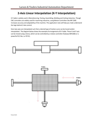
2-Axis Linear Interpolation (X-Y Interpolation)
X-Y table is widely used in Manufacturing, Testing, Assembling, Welding and Cutting industries. Though
CNC controllers are widely used for machining industries, using Motion Controllers like MP 2300
increases accuracy and adaptability of the machine. This application note will help you make understand
the logic behind 2-Axis control.
Here two axes are interpolated such that a desired type of motion curve can be traced and/or
interpolated. The diagram below shows the example of arrangement of X-Y table. These X and Y axis
can be moved using a Servo, which can be controlled by a motion controller (Yaskawa MP2300) or a
powerful PLC like, Lx-70 PLC.

2. Larsen & Toubro Industrial Automation Department
Pranav Parikh
Aim: To trace any type of X-Y curve using X-Y Interpolation.
Given: Given is the set of points which are plotted using excel or other software which is able to
plot graphs
Explanation:
Here the curve is traced by 29 points using desired combination of X and Y coordinates. These X and Y
coordinates are feed to the controller and using the interpolation logic the actual curve can be traced
using servo on the X-Y table. The accuracy of the curve depends upon the accuracy of the servo and the
scan time in the controller.

3. Larsen & Toubro Industrial Automation Department
Pranav Parikh
Logic for the Interpolation:
Steps:-
1. Finding the Angle T as shown in the figure below.
Tan(T)= O/A
= (Opposite Side)/(Adjacent Side).
= 150/100.
= 1.5
T = ArcTan(1.5)
T = 56.30˚
2. Finding the individual speeds of X and Y axis given the average or the resultant speed
between the two points:
Suppose the given average speed is 1000. So using the angle T we have the X axis speed and the
Y-Axis speed as below:
X-Speed= Cos(T)*1000
Y-Speed= Sin(T)*1000

4. Larsen & Toubro Industrial Automation Department
Pranav Parikh
By the above method a set of speeds for different x and y coordinates can be collected and can
be executed by positioning or interpolation or Phase functions in the motion controller. A
significant length of the program can be reduced if a pointer is used instead of individually
calculating the different X and Y speeds of each coordinates.
The graph as shown in the given section above can be easily executed by this method. Also a
number of other complex curves like a Spline, and a circle can be executed by a number of
minute points joined by a line connecting each other.
The results found using Yaskawa Servo and Yaskawa Motion controller were very satisfactory
and accurate.
Example of Calculation:

5. Larsen & Toubro Industrial Automation Department
Pranav Parikh
Conclusion and Proof:
The above figure shows the comparison between the actual graph being traced in MP 2300 and
the given Excel Graph, which are 100% similar. The positioning in servo always starts from Zero
or Home position.
The only thing which has to be considered very important the servo cannot be used at speed
higher than the rated speed for more time. Using servo above the rated speed continuously or
for a short distance will give unsatisfactory results.
Also the servo needs to be tuned properly depending upon the accuracy required.