The merit order is a model used in the electricity industry to determine the optimal sequence in which power plants should generate electricity based on their marginal costs. Power plants with the lowest marginal costs are dispatched first to meet demand while higher cost plants are brought online only when needed. This helps minimize production costs. Electricity prices are determined by the marginal costs of the last power plant needed to meet demand. Increasing renewable energy is shifting the merit order and lowering wholesale prices through the merit order effect. However, the model has limitations and does not reflect all long-term costs and factors influencing prices.

1. What does
MERIT ORDER
Mean
?

2. ◦In the energy industry, the term ‘merit
order’ describes the sequence in which
power plants are designated to deliver
power, with the aim of economically
optimizing the electricity supply.
◦ The merit order is based on the lowest
marginal costs.

3. These are incurred by a power plant and refer to the
cost of producing a single megawatt hour under recent
conditions. The merit order is separate from the fixed
costs associated with a power generation technology.
According to the merit order, power plants that
continuously produce electricity at very low prices are
the first to be called upon to supply power. Power
plants with higher marginal costs are subsequently
added until demand is met.

4. ◦The merit order is just one possible model for
creating a functional electricity market.
◦It assumes that power plant operators are always
trying to cover the cost of the next megawatt
hour produced; they would not produce it
otherwise.

5. Power plants with low marginal costs can
therefore offer a lower price for their electricity,
and they are in turn called upon more often than
power plants with higher marginal costs.
The merit order is designed to shed light on how
pricing works on the electricity market; it is not
a fixed "law" that coordinates the use of power
plants.

6. Electricity Price
On the electricity exchange, supply and demand
determine the prices at auction. The ‘market-clearing
price’ (MCP) is the lowest bid to buy power that is
still accepted in an auction.
The power plant with the most expensive marginal
costs
– the marginal power plant
– determines the price on the exchange for all power
plants involved.

7. The energy industry calls this price formation
mechanism ‘uniform pricing’ since all power plants
receive the same price for their feed-in, even if they
have offered different prices (in contrast to the ‘pay as
bid’ mechanism, which applies to continuous trading).
If a power plant offers a lower price than the marginal
power plant, it can generate a surplus.
This ’contribution margin’ offsets their own fixed costs.

8. Merit order effect (MOE)
Permanently declining electricity production costs – especially in renewable
power production – have caused the merit order sequence to shift, with
conventional power plants taking a position further back. The effect is quite
visible with the increasing feed-in of renewable energies (such as
photovoltaics, wind energy, or biomass).
Fluctuating photovoltaic and wind power plants with marginal costs close to
zero are advancing into the market and pushing conventional power plants
toward the end of the merit order during peak load periods. The energy
industry describes this phenomenon as the Merit Order Effect (MOE) of
renewable energies. Only the residual load – the remaining electricity
demand that renewable energies cannot cover – must be provided by
conventional power plants.

10. Criticism of the Merit Order Model
The merit order model is a static description model that is well suited for representing short-
term electricity price formation. Calculating the long-term development of electricity
prices, however, requires a market model that takes long-term effects into account. Such an
electricity market model would include factors such as operator decisions on deployment,
expansion, and decommissioning as well as fixed operational costs. The latter point is
particularly relevant: no power plant operator will want to build additional plants if selling
electricity only covers marginal costs. For example, the enormously high investment and
dismantling costs of nuclear power plants are not correctly reflected in the merit order
model. The same can be said for the total costs associated with renewable energies.
The model also requires all electricity to be sold on the electricity exchange, which does not
always happen. As an example, some plant operators consume the electricity they produce
without feeding it into the grid. Without taking these factors into account, the merit order
model can overstate the ability of renewable energies to influence prices. Therefore, the
merit order model does not fully reflect reality, leaving the full extent of the merit order
effect up for debate.

11. The Price and Value of Electricity
Electricity prices vary hour-by-hour and the implication this has for the economics of
electricity generators. By watching this video the reader will be able to understand:
•Appreciate that electricity prices may vary significantly over short intervals
•Understand how electricity prices are determined in the wholesale markets
•Get an overview of different models that explain such price setting
•Understand the “market value of electricity” and see how it relates to levelized cost

12. Electricity Price Fluctuations
Let us start with some basic empirical observations of electricity prices in liberalized
wholesale power markets, i.e. markets where generators, retailers and industrial customers
trade electricity with each other. These are the prices that determine revenues and profits of
power plants.
Prices fluctuate. In countries where wholesale markets for electricity exist, a different
electricity price is determined for short intervals of time, such as every hour, every quarter-
hour or even every five minutes. The price of electricity can vary sharply even between two
consecutive five-minute intervals.
Over the course of a week, it is not uncommon to observe intervals with high prices, low
prices, price of zero or even negative prices (which means you get paid for consuming
electricity!). For example, even though the average annual price of electricity in most
countries is somewhere between EUR 30 - 80 per MWh, it is not uncommon to observe
electricity prices above EUR 1000 per MWh during some time intervals and prices below
EUR -100 per MWh during others. This is illustrated in Figure 1, which shows the hour-by-
hour electricity prices on the so-called day-ahead market in Germany over one week.

13. Figure 1. Average hourly wholesale electricity prices in Germany during five days in 2014
Key point: Electricity prices can vary sharply depending on the time of the day/year.

14. Electricity Markets are Unique
The sharp price fluctuations on time scales as short as hours and minutes sets electricity
markets apart from other commodities. Other commodity markets, including crude oil,
natural gas, minerals, agricultural products, steel etc., also exhibit price variation, but to a
much lesser extent. For example, in 2016 the German day-ahead price of electricity was
EUR 29 per MWh on average, with a minimum of EUR -130 per MWh and a maximum of
EUR 105 per MWh.
In other words, the range of prices observed was a factor eight of the mean price. By
contrast natural gas, crude oil and coal, the three most traded energy commodities, do not
show much intra-day price variation. Annual movements in prices are also more gradual and
variations less dramatic. For example, in 2016 the price of coal increased from around USD
50 per MT to USD 100 per MT and remained between USD 75 per MT and USD 100 per
MT throughout 2017.

15. Reasons for Price Fluctuations
What makes power prices fluctuate so much more than prices of other goods? It is the
combination of three characteristics of electricity:
•The supply curve of electricity is upward-sloping
•Demand and/or supply conditions change over time
•Electricity cannot be stored economically in large volumes
It is easy to see that there is nothing special about the first two characteristics. An upward-
sloping supply curve is a feature that electricity shares with most other commodities. The
same is true for time-varying demand a just as demand for electricity is higher during the
day than at night, demand for coffee is higher in the morning hours than at noon. And yet
coffee prices on commodity exchanges do not necessarily increase during the morning
hours, while electricity prices do peak during the evening. It is the third characteristic of
electricity, i.e. non-storability, which sets it apart from other goods. Coffee beans can be
stored over night to satisfy the morning peak demand, but electricity cannot.

16. Predictable Changes:
To be more precise, we can differentiate between predictable and non-predictable prices
changes. Unexpected shocks in demand and supply can affect prices of any commodity, i.e.
the news of a pipeline failure can lead to rapid swings in the crude oil price. Unlike other
commodities, however, electricity prices fluctuate sharply between low and high periods of
demand even when the demand and supply changes predictably.
Implications of Price Fluctuations:
There are at least three important consequences of sharply fluctuating electricity prices:
•Designing electricity markets is more difficult than organizing trade of other goods, because
prices change so quickly.
•The economics of a power plant depends on when it generates electricity. Consider a hypothetical
plant that has zero fixed and zero variable cost (and hence a LCOE of zero) but produces electricity
only when prices in the wholesale markets are negative. Despite being free, no one would install
such a plant.
•Within an electrical system, it is economically efficient to build power plants based on a range of
technologies a some might generate electricity at a low cost all the time (base load plants), while
others may be designed to generate electricity only when electricity demand, and thus prices, are
high (peak load plants).

17. A Short-Run Model: Merit Order Dispatch
Merit Order Dispatch:
It is important to recognize that in the short run, the installed generation capacity in a
system cannot be increased or decreased. An important consequence of this assumption is
that fixed costs do not play any role in the production decision of power plants. Let’s think
about this. Since a given power plant has already been constructed it should be willing to
produce electricity even if the market price is infinitesimally higher than its variable cost of
generation. On the other hand it would not make any sense for the plant to generate
electricity if the market price is below its variable cost, as it would lose money on every
unit of generation. Thus in the short run marginal cost of production of electricity must
equal the variable cost of generation. We can use this idea to derive the supply curve of
electricity. This is done by simply ordering power plants in the system “by merit” i.e. by
increasing variable cost. The resulting short-term supply curve of electricity is called the
merit-order dispatch (curve) in industry parlance. A merit-order based model of electricity
prices. The “merit-order” or “supply stack” model is a helpful tool for explaining the
electricity price determination in a predominantly thermal power (coal, gas, nuclear) based
electrical system in the short run.

18. A fundamental building block of the model is the merit order curve, which serves as the short
run supply curve of electricity. The demand for electricity, in the short-run, is usually assumed
to be perfectly price-inelastic and is therefore represented by a vertical line. The market-
clearing equilibrium price is the point where the merit-order curve intersects the short-run
electricity demand (Figure 2). Why can only this point be the market-clearing price? Let’s
consider a power plant on the merit order curve that is to the left of the intersection point
(“infra-marginal power plants”): this plant earns a positive amount, equal to the difference
between the market clearing price and its own variable cost, and will thus forgo profit by not
generating electricity. Now consider a plant to the right of the market-clearing price (“extra-
marginal plants”): this plant would incur a loss on every unit of generation and thus would not
rationally generate electricity.
The last power plant to generate electricity (“marginal plant”) is the one whose variable cost is
equal to the market-clearing price, and it will generate with-out incurring any profit or loss. In
summary, in the short run it is optimal to “dispatch” all plants to the left of the marginal plant
on the merit order dispatch and keep those to the right out of production, and the only price that
ensures that load is exactly served is the variable cost of the marginal power plant.

19. Figure 2: The merit-order model of price determination in a certain hour
Key point: Prices are determined by the intersection of demand and supply.

20. Fluctuating load. The merit-order model can be used to understand why prices vary. One reason is that
electricity demand varies due human activity and needs. If demand drops, the clearing price is lowered, and
vice versa (Figure 3).
Figure 3: The merit-order model of
price determination with fluctuating load
Key point: Prices vary with change
in electricity demand.

21. How to account for the Renewables?
Wind and solar power have zero variable costs and would always fall at the extreme left of the
supply curve. However, incorporating these renewable energy generators into the merit-order
model is somewhat awkward. This is because, unlike other technologies the availability wind
and solar power varies significantly even in the short run. Given these special characteristics,
there are two options of integrating wind and solar power. The first is to group them with the
thermal generators. This makes sense because that is what they are: suppliers of electricity.
However, because the underlying resource varies, the supply curve would then also shift from
hour to hour, which means we would need to draw a different diagram for every hour. The other
option is to treat wind and solar generation as “negative load” and replace the load curve with
the net (or “residual”) load curve. This allows us to use a supply curve that is stable and a
residual demand curve that varies over time.
Dynamic perspective. Figure 2 shows power plant dispatch and the market-clear pricing for one
specific hour. Figure 4 shows net demand (consumption net of wind and solar generation) as
well as the electricity price for the same five days. It becomes evident how clearly price and
residual demand are correlated.

22. Figure 4: Electricity demand and wholesale price hour-by-hour during one week
Key point: During times of high net demand, prices tend to be high. As a consequence price
fluctuates with demand.

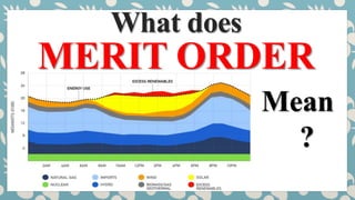
23. Figure 5 shows the generation mix by technology during the same week. During periods with low residual
demand, technologies with low variable costs are dispatched and at times of high residual demand, high-cost
generators also get dispatched.
Figure 5: The electricity generation mix by the hour during five days
Key point: The dispatch of generation technology changes over time.