1. etroleum fuel and petrochemical production from oil refin-
eries in 2006 did not match new demand, causing jumps
in prices for gasoline, jet fuel, diesel, heating oil and petro-
chemicals worldwide. Prudently relaxing refinery constraints is an
effective way to increase production and profit.
Refinery limits are usually quoted as maximum feed rates to
major processes like fluid catalytic cracking (FCC) and catalytic
reforming (CR) for gasoline; hydrocracking (HCU) and delayed
coking (DCU) for jet and diesel; hydrodesulfurization (HDS)
for sulfur removal; and crude distillers (CDUs) for crude oil sep-
aration. But unit feed can always be increased above the name-
plate maximum by reducing operation severity and hence, yield
or quality of valuable products, causing a profit decline. Rather
than a hard feed limit, an economic best feed rate exists. Profit
versus feed rate has a hill or tent shape. Further, the best feed rate
varies with feed composition like density or sulfur content as
well as product–crude price differentials. Real process limits are
determined by mechanical, thermal and chemical phenomena
within specific equipment component bottlenecks throughout
these major refinery processes. Operating setpoints are specified
within these limits to account for transients and risks but their
best-practice determination is empirical and controversial.
Vapor velocity. Many refinery vessels are, or should be, capac-
ity limited by the velocity of vapors within them. As their feed
increases, profit generation increases until the vapor velocity
limit is reached, beyond which detrimental phenomena suddenly
occur, curtailing profit severely. The profit rate versus steady-
state velocity is shaped like an asymmetric tradeoff tent, peak-
ing at the limit and often exhibiting a discontinuous cliff there.
Chemical engineers have good nonlinear empirical models for
the financial credits for approaching limits and for the onset of
the detrimental phenomena behavior, but the latter are not exact
and do not quantify the financial consequences very well when
limits are exceeded. Limit and setpoint setting are controversial
and reviewed by management.
FCC. Well-designed FCCs are usually limited by regenerator
vapor velocity; if excessive, entrained catalyst cannot be returned
through recovery cyclone dip legs and serious losses to atmo-
sphere result, or O2 breakthrough causes harmful afterburning.
Well-designed FCCs run with high catalyst circulation and low
pressure drop (2–4 psi) across a regenerated-catalyst slide valve.
If this SVDP can be reduced, air blower discharge pressure drops
giving it more air capacity, or wet gas compressor suction pressure
increases giving it more capacity; both are economically attractive.
If fluidized catalyst rate is too high the pressure drop goes below
zero and catalyst flow reverses, sending valuable feed to destruc-
tion. In 1996, one 100 kbpd FCC had a credit for reducing SVDP
1 psi of $1 kk/yr, but the loss was $200 k/reversal incident. So
a profit tradeoff tent between production and reversals exists for
catalyst velocity.
CDU. CDUs are crude oil distillation columns contain-
ing upward flowing vapors fractionated by downward flowing
liquids for separating and purifying components. When either
vapor or liquid rates become excessive, flooding ensues and
separation declines rapidly. All distillation columns are capac-
ity limited by flooding and vapor velocity. All processes have
distillation columns. Vacuum units recover valuable gas oil
from residue. They are limited by residue mist contamination
when velocity at their base is excessive at low pressure. Chemical
engineers use Stokes’ Law (friction force on drops overcomes
gravity force) to predict liquid entrainment in up-flowing vapor.
So a profit tradeoff tent between capacity and flooding exists for
distillation vapor velocity.
Vapor-liquid separators. Refineries are full of pipes contain-
ing vapor/liquid mixtures that go to vessels called separators which
reduce velocity, allowing liquid to coalesce and leave at the bottom
and vapor to leave overhead. Downstream pumps require vapor-
free liquid to avoid cavitation and compressors require liquid-free
vapor to avoid piston or blade damage. If either output stream
has much mixture, severe damage results. Each separator has a
vapor velocity limit for proper separation. Stokes’ Law estimates
excessive mist in the vapor exit. So a profit tradeoff tent between
capacity and damage exists for separator velocity.
Reactors. Most refinery reactors—CR, HCU and HDS
among them—are reaction rate limited in fixed-volume catalyst
beds. DCU thermal crackers are limited by drum size. The extent
of conversion to valuable products or sulfur removal declines as
vapor residence time decreases, i.e., at excessive velocity. So a
profit tradeoff tent between capacity and yield exists for reactor
velocity.
Furnaces. Most processes have a furnace to supply needed
Set vapor velocity setpoints profitably
Use Clifftent principles to account for operating limit tradeoffs
and risk to substantially improve financial performance
P. R. LATOUR, CLIFFTENT Inc., Houston, Texas
P
PROCESS CONTROL AND INFORMATION SYSTEMS SPECIALREPORT
October 2006 issue, pgs 51–56
Used with permission.
www.HydrocarbonProcessing.com
Originally appeared in:
Article copyright © 2006 by Gulf Publishing Company. All rights
reserved. Not to be distributed in electronic or printed form, or posted
on a Website, without express written permission of copyright holder.
HYDROCARBON PROCESSING OCTOBER 2006

2. SPECIALREPORT PROCESS CONTROL AND INFORMATION SYSTEMS
heat. As the heat duty of a furnace increases, its burner fuel vapor
velocity increases and firebox flame grows. When the flame begins
to impinge on hydrocarbon-carrying tubes, ruptures eventually
occur. So a profit tradeoff tent between capacity and damage exists
for heater fuel velocity.
Compressors. Most processes have a large compressor. As inlet
vapor velocity increases, the horsepower required to compress to
a fixed discharge pressure increases, leading to overload of the
compressor and its driving motor or turbine. Many olefin plants
are capacity limited by process gas compressors. Many FCCs are
capacity limited by wet gas compressors or air blowers. Many
HCUs are limited by recycle H2 compressors. Many cryogenic
demethanizers in olefin plants and natural gas plants are limited
by refrigeration compressors. So a profit tradeoff tent between
capacity and damage exists for compressor inlet velocity.
Absorbers. Impure gas enters the bottom of these vessels and a
liquid that absorbs some of the impurities enters the top. The gas
is scrubbed of impurities and they leave in the bottom liquid as
the purified gas leaves the top. However, at high velocity, absorb-
ing liquid mist is entrained and exits with the purified vapor, caus-
ing unacceptable results. Stokes’ Law estimates the entrainment
carryover. If the rich absorbent stripper is limited, recovered lean
absorbent retains impurities so its absorbing power declines and
feed or purified gas must be flared.
Amine absorbers are used in all refineries to recover H2S for
sulfur removal. Absorbers are increasingly used to separate meth-
ane from hydrocracker recycle hydrogen;1 methane from high-
nitrogen, low-Btu natural gas;2 and olefins from alkanes.3 CO2
absorbers are needed to purify CO + H2 from Fischer-Tropsch
synthesis gas. One large coal-based refinery/petrochemical com-
plex was limited by its CO2 absorber and throttled its entire coal
conveyor, gasifier and synthesis train to steady vapor velocity
within CO2 absorber limits for maximum production. A control
system designed to reduce vapor velocity variance could allow 3%
higher average production within CO2 absorber limits, worth >$5
kk/year. So a profit tradeoff tent between capacity and flaring
exists for absorber velocity.
CV/KPI. For these reasons, vapor velocities are important con-
trolled variables (CVs) and key performance indicators (KPIs) of
refinery processes. But they are quite variable and not directly
measurable. Remember the perfect gas law, PV = nRT, from
high school chemistry? This means vapor volume or velocity,
V, depends on pressure, P, temperature, T, and composition
molecular weight, n. (R is the universal gas constant.) So velocity
can be held steady near its limit by adjusting either P, n or T in
the face of uncontrolled variations in the other two. Pressure and
temperature are much easier to measure and adjust than velocity.
When composition is known, velocity is inferred by V = nRT/P.
Velocity variations. Since velocity is inherently variable by
the gas law when n, T and P change, and since it is difficult to
measure directly, there is considerable uncertainty about its actual
instantaneous value and its approach to limit. Further, there is
considerable uncertainty in the actual velocity value from chemi-
cal engineering models that signifies the onset of the damaging
behavior.These uncertainties are quantified in the statistical distri-
bution of velocity historic data trends and operator experience.
Setpoint problem. All of this is to explain important ways refin-
eries are run to maximize profit: control vapor velocity tightly and
adjust its average in the neighborhood of real limits, optimally. How-
ever, setting the limits and setpoint tolerance has been an art; there
was no rigorous mathematical procedure for managing the risk to set
them for maximum expected net-present-value profit until 1996.4 If
the penalty of violation is deemed large and variance high, setpoints
are naturally set safely below limits. If the credit for approaching is
deemed large and variance low, setpoints are naturally set tightly near
limits. Not much has been published on modeling the financial con-
sequences of violating equipment limits and quality specs, identified
as the area of Re4, Hazop and abnormal situations. Whenever the
actual economic sensitivities and variance differ from those assumed,
the current setpoint is not optimum, and profit is lost. This is basic
risk management balancing of uncertain tradeoffs that people do
every day, like setting your car speed.
Clifftent analysis4–12 was published in 1996 to determine the
financial merit of reducing CV variance to quantify the value of
improved dynamic performance of process control systems. It
takes the statistical distribution and the steady-state profit tradeoff
tent, integrates them and provides a smooth hill profit function
and top value that accounts for variance uncertainty. It provided
the HPI (and all industry) with the rigorous way to measure value-
added performance of process control and information technology
TABLE 1. Clifftent demo—CO2 absorber load
Problem definition, input:
1. Unit profit function. Below Above
Slope 60.000 –50.000
Curvature –100.000 –100.000
Specification limit 1.050 Type: max.
Unit profit at spec. 3.000 Cliff: –56.000
Production capacity, units/time: 200.0
2. Measured data distributions for time period:
Mean Std. dev.
Base case 0.950 0.060
Improved case — 0.040
Solution, output:
1. Std. dev. = 0.060 Mean Time profit Crude
Base–start 0.950 580.978 181.0
Base–optimum 0.940 581.251 179.0
Change, amount –0.010 0.272 –1.9
Change, pct. –1.101 0.047 –1.1
2. Std. dev. = 0.040
Base–start 0.940 584.972 179.0
Base–optimum 0.967 586.941 184.2
Change, amount 0.027 1.970 5.1
Change, pct. 2.911 0.337 2.9
3. Comparison–dynamics only:
Base–optimum 1 0.940 581.251 179.0
Base–start 2 0.940 584.972 179.0
Change, amount 0.000 3.721 0.0
Change, pct. 0.000 0.640 0.0
4. Comparison–optimums:
Base–optimum 1 0.940 581.251 179.0
Base–optimum 2 0.967 586.941 184.2
Change, amount 0.027 5.691 5.1
Change, pct. 2.911 0.979 2.9
5. Comparison–total:
Base–start 1 0.950 580.978 181.0
Base–optimum 2 0.967 586.941 184.2
Change, amount 0.017 5.963 3.2
Change, pct. 1.777 1.026 1.8
HYDROCARBON PROCESSING OCTOBER 2006

3. SPECIALREPORT PROCESS CONTROL AND INFORMATION SYSTEMS
(IT) investments for computer-integrated manufacturing (CIM)
by converting CVs/KPIs to profit indicators. It also provided the
HPI with the rigorous way to set linear program (LP) constraint
values and operating setpoint tolerances near limits with CV profit
meters. This feature alone generates great value. Clifftent should
be used to frequently determine the best vapor velocity settings for
all important refinery processes. The keys are accurate economics
and short-term variance forecasts.
CO2 absorber load example. A simplified example of a
CO2 absorber limiting capacity of a synthetic crude oil plant is
offered to illustrate the Clifftent method application. There is a
close analogy to amine H2S absorbers in conventional refineries
and the vapor velocity limits in all process equipment.
Suppose the maximum steady-state limit is known to be 1.05
kkncm/day CO2 absorbed by hot potassium carbonate, deter-
mined from feed–lean off-gas, 8.05–7.00. Management has speci-
fied a setpoint target of 1.00, but the typical mean achieved by
operators is only 0.95. The standard deviation, sd, of hourly data
is about 0.006 kkncm/d, rather steady, but the sd of daily/weekly
data is about 0.06 kkncm/d, much more variable. An improved
measurement, modeling, control, risk management, information
system claims to be able to reduce sd by 1/3, from 0.06 to 0.04.
So base case sd = 0.06; improved case sd = 0.04.
Syncrude refinery maximum theoretical capacity at 1.05
absorber load limit = 200 kbpd. Typical capacity at 0.95 is 200
 0.95/1.05 = 181.0 kbpd. Assume refinery unit profit = $3/bbl
crude (this allows graphing but does not affect benefits). So zero
variance maximum profit at 1.05 is 200  3 = $600 k/day.
The Clifftent profit function is set by three numbers: profit
sensitivity slopes on either side of the 1.05 absorber limit and any
penalty cliff at that limit.
For the left side credit slope approaching the limit we increase
crude 0.1% for a 1.0% increase in CO2 absorbed. The profit tent
slope is 0.1  $3 bbl crude  200 kbpd/kkncm/d = $60 k/kkncm
CO2. The right side penalty slope exceeding the limit is found to
be –$50 k/kkncm.
For the cliff, assume an incident when the 1.05 limit is
exceeded; potassium carbonate absorbent is saturated in CO2
because the absorber had been running near its 1.05 maximum.
Normal CO2 breakthrough causes off-gas to flare. The operator
must cut crude 10%  200 kbpd = –20 kbpd, to 180, for 8 to
36 hours, 16 hours typical. An additional penalty arises because
the operator must flare 15% of absorber feed for 16 hours; it
costs $20/kncm. So cliff = –20 kbpd  $3/bbl  16/24 – 0.15
 8 kkncm/d  $20/kncm  16/24 = –40 – 16 = –$56 k/d. We
include some nonlinear model curvature = –$100 k/d/(kkncm/d)2
on both sides. Profit is k$/d. Results are in Table 1.
Start with sd = 0.06 and mean = 0.950; the optimum mean is
found to be 0.940 and the profit gain to move down 0.010 and
drop crude from 181.0 to 179.0 is $272/day. This profit is the net
gain created by setpoint optimization from reduced limit viola-
tions that outweigh losses from lower production.
Next, reduce sd to 0.04 by control investment.The new optimum
mean is 0.967 and corresponding crude is 184.2.There are two profit
gains: $3,721/day from reduced sd at the starting optimum mean
0.940 due to investment, and $1,970/day from moving the mean up
to 0.967 due to setpoint optimization, for a total of $5,691/day when
Clifftent and control/IT systems work together. The first $3,721
gain comes from less low load and low production occurrences and
less excess load flaring.The second $1,970 gain comes from a higher
production credit exceeding a higher flaring penalty.
From the base case 0.950, sd = 0.06, to improved control at
0.967, sd = 0.04, the profit gain is $5,963/day, 3,721/5,963 =
62.4% of which is due to variance reduction by control/IT. Gen-
erally we find it is about 50%; setpoint optimization generates
the other 50%.
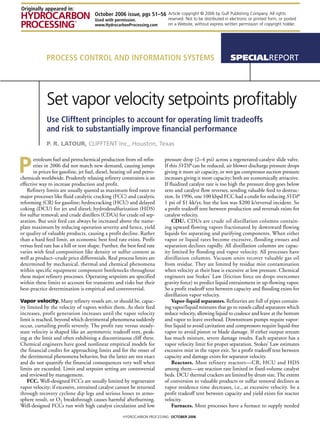
Fig. 1 shows the starting position. The base blue distribution
has mean = 0.95; the improved green distribution has mean = 0.94.
The red profit function is provided. As the blue distribution slides
from left to right, profit changes according to the pink hill with the
top at 0.94. As the green distribution slides from left to right, profit
changes according to the brown hill with the top at 0.967. Fig. 2
shows the same curves with the improved green distribution at its
hill top mean of 0.967. These hills are CV/KPI profit meters.
If perfect control of absorber load, sd = 0, could be achieved for
extended periods, the theoretical optimum mean is 1.05, crude
rate = 200 kbpd and added profit = 600.000 – 586.941 = $13.059
k/day, or 13.059/200 = $0.065/bbl crude. Of course, such per-
fection is infinitely expensive to achieve, hence unattainable. But
the cost and performance claim of other ideas for improvement
to capture some of this potential can be benchmarked for greater
profit generation by rerunning Clifftent.
Suppose the overload can be quickly mitigated by operator
���� ���� ����
�����������������������
���� ���� ����
���
���
���
���
���
���
���
��
��
��
��
��
�
�
���
���
���
���
���
���
���
��
��
��
��
��
�
�
���
���
���
���
���
���
���
Absorber start; move 0.95 to 0.94.FIG. 1
���� ���� ���� ���� ���� ����
���
���
���
���
���
���
���
��
��
��
��
��
�
�
���
���
���
���
���
���
���
��
��
��
��
��
�
�
���
���
���
���
���
���
���
�����������������������
Absorber improved; move 0.94 to 0.967.FIG. 2
HYDROCARBON PROCESSING OCTOBER 2006

4. training or alarm systems, reducing the cliff 50%, from –$56 to
–$28 k/day. The optimum mean is found to be 0.960 and the
profit gain to move up 0.010 and increase crude from 181.0 to
182.9 is $193/day.
Next, reduce sd to 0.04 by better control. The new optimum
mean is 0.981 and corresponding crude is 186.9. There are two
profit gains: $3,620/day from reduced sd at the starting optimum
mean 0.960, and $1,030/day from moving the mean up to 0.981,
for a total of $4,650/day.
From the base case 0.950, sd = 0.06, to the improved control
at 0.981, sd = 0.04, the profit gain is $4,843/day, 3,620/4,843 =
74.7% of which is due to variance reduction by control.
Fig. 3 shows the starting position. The base blue distribution
has mean = 0.95; the improved green distribution has mean
0.96. The red profit function is provided as above. As the blue
distribution slides from left to right, profit changes according
to the pink hill with the top at 0.96. As the green distribution
slides from left to right, profit changes according to the brown
hill with the top at 0.981. Fig. 4 shows the same curves with the
improved green distribution at its hill top mean of 0.981.
Important observations. Several observations can be made.
Reduced variance about the same mean makes money. Modeling
the financial penalty of limit violation is as important as the credit
for approaching the limit. If any input value to proper setpoint set-
ting is incorrect, the plant will be operated suboptimally; money
is lost. If limit violation penalties can be mitigated and setpoints
adjusted accordingly, profit increases. If profit sensitivity slopes
are more horizontal, the KPI is less important and profit increases.
The only thing control/IT operators can do is modify the position
and shape of CV/KPI distributions like vapor velocity. They man-
age risk by proper alignment under the profit Clifftent. Clifftent
graphs are profit meters for each CV/KPI. Other consequences for
plant operation management have been published.4, 5, 10, 11, 15
Significance. Clifftent provides an easy way for refiners who
know their processes, particularly the economic consequences for
violating properly set limits, to set process limits and setpoints
properly. Modern model and IT systems should provide the key
financial sensitivities that constitute the Clifftent profit function
for each CV/KPI. Vapor velocity examples in a host of refinery
processes illustrate the application scope. While not all vapor
velocity or CV/KPI tradeoffs are as sensitive as this syncrude refin-
ery constrained CO2 absorber example, many will provide signifi-
cant profit sources. Product quality specifications are fertile for
Clifftent optimizations too.4, 5, 7
Reducing vapor velocity variance by modern control, modeling
and IT systems generates profit >$1/bbl crude refined for operat-
ing companies that do the CIM business right.6, 8–15 Clifftent is
needed to prove it. Another profit >$1/bbl crude refined is gener-
ated by using Clifftent to set other optimal setpoints.4, 5, 15
Just as one should thoroughly understand scoring before ath-
letic competition, one should never embark on substantial IT
investments without a clear, rigorous performance score keeper;
Clifftent provides that profit measurement. In fact it allows tech-
nology solution providers that know the CV/KPI variance reduc-
tion capability of their systems to license for a fair percentage of
sustainable performance using shared risk-shared reward (SR2)
methods, to mitigate customer investment risk.5, 6, 15 This explains
the demise and key to the rise of process control.15 As the tenth
anniversary of Clifftent’s disclosure approaches,4, 7 the author
has been astonished by the lack of interest from suppliers, plant
managers and academia in measuring control system financial
performance. One would think they would be interested in the
value of their work.
If people adopted Clifftent principles for all significant deci-
sions, the value to humanity would far exceed Einstein’s discovery
of general relativity and E = MC2 because there is no down side.
Civilization progresses by adding value when human intelligence
is deployed to mitigate risk by proper goal setting, analysis, mod-
eling, forecasting, synthesis and execution. Good drivers set their
speed setpoints this way.
Are your refinery vapor velocities tightly controlled at setpoints
accurately reset to maximize expected net-present-value profit?
Regularly? Are you accounting for upcoming uncertainty prop-
erly? Do you know the profit lost if you don’t, and the profit
gained if you do? Are there any better ways to set setpoints? HP
LITERATURE CITED
1 Mehra, Yuv R. and Al-Abdulal, Ali H., “Hydrogen Purification in
Hydroprocessing,” Saudi Aramco Journal of Technology, Fall 2005, pp. 2–8 and
Paper AM-05-31, NPRA Annual Meeting, March 2005. See www.aet.com.
2 Mehra, Yuv R., “Guidelines Offered for Choosing Cryogenics or Absorption
for Gas Processing,” Oil and Gas Journal, March 1, 1999, V97, n99, p. 62.
3 Mehra, Yuv R., “Absorption Process for Recovering Ethylene and Hydrogen
���� ���� ����
�����������������������
���� ���� ����
���
���
���
���
���
���
���
��
��
��
��
��
�
�
���
���
���
���
���
���
���
��
��
��
��
��
�
�
���
���
���
���
���
���
���
Absorber cliff 50% start; move 0.95 to 0.96.FIG. 3
���� ���� ����
�����������������������
���� ���� ����
���
���
���
���
���
���
���
��
��
��
��
��
�
�
���
���
���
���
���
���
���
��
��
��
��
��
�
�
���
���
���
���
���
���
���
Absorber cliff 50% improved; move 0.96 to 0 0.981.FIG. 4
HYDROCARBON PROCESSING OCTOBER 2006

5. SPECIALREPORT PROCESS CONTROL AND INFORMATION SYSTEMS
from Refinery and Petrochemical Plant Off-Gases,” US Patent 5,546,764,
August 20, 1996.
4 Latour, P. R., “Process control: CLIFFTENT shows it’s more profitable than
expected,” Hydrocarbon Processing, V75, n12, December 1996, pp. 75–80.
5 Latour, P. R., “CIMFUELS,” bi-monthly contributing editorial, FUEL
Reformulation, September 1995–February 1998.
6 Latour, P. R., “Does the HPI do its CIM business right?” HPInControl
guest columnist, Hydrocarbon Processing, V76, n7, July 1997, pp. 15–16 and
“Optimize the $19-billion CIMfuels profit split,” V77, n6, June 1998, pp.
17–18.
7 Latour, P. R., “CLIFFTENT: Determining Full Financial Benefit from
Improved Dynamic Performance,” Paper C01,Third International Conference
on Foundations of Computer-Aided Process Operations, Snowbird, Utah,
July 5–10, 1998. Proceedings published in AIChE Symposium Series No.
320, V94, 1998, pp. 297–302.
8 Latour, P. R., “Decisions about risk reduction,” letter to editor, Hydrocarbon
Processing, V80, n6, June 2001, p. 39.
9 Latour, P. R., “Quantifying financial values,” HPInControl guest columnist,
Hydrocarbon Processing, V80, n7, July 2001, pp. 13–14.
10 Latour, P. R., “Why Invest in PROCESS CONTROL?” CONTROL, Vol. XV,
n5, May 2002, pp. 41–46.
11 Latour, P. R., “Why tune control loops? Why make control loops?” editorial,
Hydrocarbon Processing, V81, n9, Sept 2002, pp. 11–12.
12 McMahon, T. K., “CLIFFTENT for Process Optimization,” CONTROL,
V17, n12, Dec 2004, p. 66.
13 Latour, P. R., “Role of RIS/APC for Manufacturing RFG/LSD,” National
Petroleum Refiners Association 1994 Annual Meeting, San Antonio, Texas,
March 21, 1994.
14 Latour, P. R., “Mission: Plan to Use RIS/APC for Manufacturing RFG/LSD,”
Fuel Reformulation, V4, n4, July/August 1994, p. 20.
15 Latour, P. R., “Demise and keys to the rise of process control,” Hydrocarbon
Processing, V85, n3, March 2006, pp. 71–80, and letters to editor, Process
Control, Hydrocarbon Processing, V85, n6, June 2006, p. 42.
Pierre R. Latour is an independent consultant specializing
in measuring financial performance of HPI process control and
information systems (Clifftent) to support shared risk-shared reward
(SR2) licensing of profit sustaining solutions, and is president of
CLIFFTENT Inc. He was a vice president of business development,
marketing, engineering, project implementation and consulting at Aspen Technology,
Dynamic Matrix Control Corporation, Setpoint and Biles & Associates. Dr. Latour was
chairman of Setpoint Japan and cofounded the last four firms. He was an engineer
at Shell Oil and DuPont and served as captain, US Army, NASA, Houston. Dr. Latour
holds a BS degree from Virginia Tech and a PhD degree from Purdue University, both
in chemical engineering. He has worked on contracts for 50 HPI companies world-
wide on most processes like ACU, FCC, HCU, DCU, olefins, aromatics, blending,
gasification, polymers, distillation and utilities. Dr. Latour has authored 65 publica-
tions and was cimfuels editor for Fuels. He is a registered PE in California and can be
contacted at e-mail: clifftent@hotmail.com.
Article copyright © 2006 by Gulf Publishing Company. All rights reserved. Printed in U.S.A.
Not to be distributed in electronic or printed form, or posted on a Website, without express written permission of copyright holder.