J o u r n a l o f
Business FOrecasting
	SOP in the
Service Industry
	 By Patrick Bower
2 0 1 5 | s u m m e r 	 V o l u m e 3 4 | I s s u e 2
292619 Supply-Neutral versus
Unconstrained Demand
By Larry Lapide
SOP:
OrganicValley’s Journey
By Beth Wells
Cleanse Your Historical
Shipment Data? Why?
By Charles W. Chase, Jr.
4
Institute of Business
Forecasting  Planning
Institute of Business
Forecasting  Planning
w/ Leadership Forum  1-Day Forecasting  Planning Tutorial
business
Planning 
Forecasting
B e s t P r a c t i c e s C o n f e r e n c e
tel: +1.516.504.7576 | email: info@ibf.org | web: ibf.org /1510.cfm
REUNION RESORT, A WYNDHAM GRAND RESORT | ORLANDO, FLORIDA  USA | october 18–21, 2015
SILVER
PACKAGE
only $1399(USD)
When you mention this ad
Register
Today!
testimonials
To view Table of conTenTs and purchase
Visit: www.ibf.org/FUNDAMENTALS.CFM
tel: +1.516.504.7576 | email: info@ibf.org | web: www.ibf.org/FUNDAMENTALS.CFM
testimonials
2nd Edition–2015
Michael Wachtel
Vice President
of Supply Chain
l’oreal
“Whether you are just getting
into the vocation or an executive
looking to take your Demand
Planning to the next level,
make sure to pick up this book
to ensure your organization is
heading in the right direction.”
Jay Nearnberg
Director, Global Demand
 SOP Excellence
novarTis
consuMer healTh
“I would recommend the book
to any Demand Planning prac-
titioner as a practical way of
maintaining current know-
ledge in this rapidly changing
field.”
Curtis Brewer
Head of Forecasting–
Environmental
Science USA,
baYer cropscience
“This work is a great foundational
book for anyone working in the
Forecasting and Demand arena.”
Mark Covas
GroupDirector,PlanningCOE
coca-cola
coMpanY
“This is a ‘How to Book’ every
Forecaster and Planner should
have on their desk!”
Todd Gallant
Senior Director,
Timberland Operations
vf corporaTion
“ Leaders will find it perfect to
educate their teams, peers, and
management on critical busi-
ness processes that keep the
supply chain in motion. This
book will be a must read for
members of my team.”
Chaman L. Jain
Editor-in-Chief
Evangelos O. Simos
Editor, International Economic Affairs
U. Rani
Business Manager
Judy Chan
Graphic Designer
Manuscripts Invited
Submit manuscript to:
Dr. Chaman L. Jain
Tobin College of Business
St. John’s University, Jamaica, NY 11439
jainc@stjohns.edu
Subscription Information
Change of address requests
for subscription, and other
correspondence should be
addressed to:
Journal of Business Forecasting
350 Northern Boulevard, Suite 203
Great Neck, New York 11021 USA
Tel:	+1.516.504.7576
email: info@ibf.org
Website: http://www.ibf.org
ID No: 11-263-2688
Published Quarterly
Domestic	$95
Foreign	$120
© Copyright 2015
by Journal of Business Forecasting
ISSN 1930-126X
Editorial Review Board
George C. Wang
Consultant
New York, NY
Mark J. Lawless
Consultant
Braintree, MA
Paul Sheldon Foote
Cal. State University–Fullerton
Fullerton, CA
3 Answers to Your Demand Planning
and Forecasting Questions
4 SOP in the Service Industry
By Patrick Bower
19 Supply-Neutral versus Unconstrained Demand
By Larry Lapide
26 SOP: Organic Valley’s Journey
By Beth Wells
29 Cleanse Your Historical Shipment Data? Why?
By Charles W. Chase, Jr.
34 Will High Risk Events Trigger a Recession?
By Evangelos Otto Simos
40 The U.S. Economy to Bounce Back in
Second Quarter
By Nur Onvural
48 IBF Calendar 2015
J o u r n a l o f
Business ForecastinGV o l u m e 3 4 I s s u e 2 | s u m m e r 2 0 1 5
2	 Copyright © 2015 Journal of Business Forecasting | All Rights Reserved | Summer 2015
[ Q ]	 How do companies arrive at a“forecast that matters?”
[ A ]	 A forecast that matters is the one that gives an error,
which is tolerable. How much error can be tolerated depends
on the company’s ability to adjust to the error and the cost
of error. If the lead time is too long, the company cannot
adjust quickly to the error, particularly, in the case of under-
forecasting. How much the error will cost also matters. The best
thing, therefore, is to generate ex post forecasts for a number
of periods to determine how much error can be expected. Try
to find ways to improve it further if necessary. If not, it has to
be compensated with additional inventory, or customer service
has to be compromised.
[ Q ]	 I am working on a portfolio review of a consumer
products company for the Executive SOP meeting. I want to
know how to go about deciding whether to keep a product or
eliminate it?
[ A ]	 The decision should depend on how much a product is
costing and how much revenue and profit it is generating. If it is
not providing enough profit, you may decide to discontinue it.
Cost comes in terms of holding inventory as well as in producing
it. The production cost usually goes up when products are
produced in smaller quantity. Furthermore, at times, we may
have to go beyond the profit generated by a product. Instead,
go by the profit generated by other products as a result of it.
I have seen cases where a customer places larger orders for a
product year in and year out simply because he/she cannot
get it anywhere else. If you discontinue it, you may lose that
customer too.
[ Q ]	 We are in the fashion industry. Although we operate on
a make-to-order model, we still wind up with huge inventory.
Can you offer a solution?
[ A ]	 There are three things to do, or are worth looking into:
1.	 Seeifthereisanopportunityforproductrationalization.
SKUs that yield little or no profit are good candidates
for elimination. Very often elimination of some SKUs
does not impact much the total revenue or profit.
2.	 Review point-of-sales data weekly. This will help in
determining which SKUs are moving and which ones
Answers toYour Demand Planning
and Forecasting Questions
are not, thereby helping to align better inventory with
demand.
3.	 Buy less raw material, buy more frequently. Doing so
will increase the cost, but it will pay in the long run.
[ Q ]	Where in the organization would you recommend
statistical forecast be prepared and why—at the headquarters
by the central Global Demand team or locally by the market
teams?
[ A ]	 Forecasts should be prepared locally (by each country
or region), and then consolidated by the headquarters. They
should be prepared locally because they know their data and
market better than anyone else. They should be consolidated,
refined, and adjusted by the Global Demand team at the
headquarters, because they would be impartial. They may
detect a bias or issue ignored/overlooked by the local team.
[ Q ]	 In calculating forecast error, should we divide error by
actual or forecast?
[ A ]	 We should divide error by the actual simply because we
want to know how forecast deviated from the actual, not how
actual deviated from the forecast.
[ Q ]	 Do small companies need an SOP process to drive
financial planning/budgeting?
A. The ultimate goal of the SOP process is to drive financial
planning/budgeting, which is needed both for large and
small companies. So, the process is not limited to the size of a
company. It will benefit every company.
[ Q ]	 Is there any special metric for measuring forecast error of
slow moving products?
[ A ]	 I am not aware of any special metric for measuring error
of slow moving products. The only thing is here we should
compute error over a longer period of time.
Happy Forecasting!
Chaman L. Jain, Editor
St. John’s University | Jainc@Stjohns.edu
	 Copyright © 2015 Journal of Business Forecasting | +1.516.504.7576 | www.ibf.org | All Rights Reserved | Summer 2015	 3
SOP in the Service
Industry
By Patrick Bower
E x ecu t i v e S ummar y | Countless manufacturing companies have tackled the challenge of implementing SOP.
Those that have nurtured the process to maturity reap considerable benefit streams. However, service sector companies—
with no products to build, no inventory to ship, and no shelves to stock—have missed out on similar advantages simply
because there’s no unified process model for mirroring the integrated planning strategies of the manufacturing world into
the realm of service.
4	 Copyright © 2015 Journal of Business Forecasting | +1.516.504.7576 | www.ibf.org | All Rights Reserved | Summer 2015
O
ne of the more interesting
informal discussion topics at
business forecasting and supply
chain conferences centers around a
simplequestion:CouldtheSOPprocess
be leveraged in non-product service
industries such as (but not limited
to) municipal government, school
systems, universities, and correctional
institutions, or in non-public service
sector organizations such as consulting,
banking, and financial services? Over
time, these informal debates became
personally intriguing, leaving me
scratching my head and wondering—
could there be a better way to plan the
service sector, and could SOP be the
answer to an unasked question?
With my curiosity aroused, I set
about looking for SOP processes in
the service sector, focusing my personal
lens on examining planning processes
of all sorts and types. After more than
a decade of casual observation, I offer
with certainty that there are forecasting
and planning processes with varying
degrees of maturity and efficacy being
used in most service organizations. I
am also aware that only a handful of
these service-sector planning processes
are as sophisticated as a mature SOP
process, and none these were actually
called SOP. As I prepared for this article,
I deepened my search, and with the
exception of the occasional informal
debate, I found only scant treatment of
service-based SOP in literature such
as technical journals or white papers.
Service-based SOP it seems, is about as
elusive as the Loch Ness Monster.
SOP PROCESS
It may be useful to step back for a
momentanddefinetheSOPprocess.For
the uninitiated, SOP is a rigorous, multi-
step, cross functional, mid- to long-range
planning process model that is heavily
deployed in manufacturing companies.
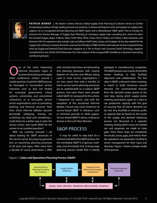
TheSOPprocessusesaseriesofmonthly
review meetings to help facilitate
alignment and collaboration. The first
step in SOP, a demand review meeting,
is meant to build consensus around
demand. The unconstrained forecast
from the demand review passes to the
next step, during which supply review
meeting participants agree on a plan to
use productive capacity with the goal
of assuring that all future demand can
be met. Any shortfalls in revenue, profit,
or capacity that are based on the results
of the supply and demand balancing
process are discussed in a separate
meeting, during which issues are hashed
out and proposals are made to close
gaps. Once these steps are completed,
the results, issues, gaps, and metrics from
the operations are presented monthly to
senior management for their input and
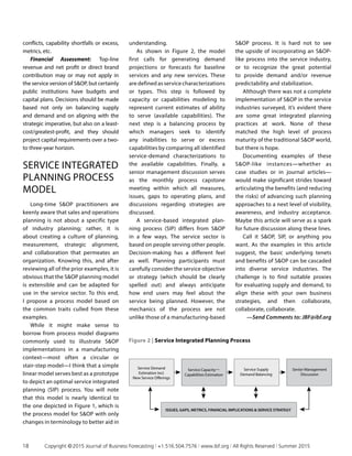
direction. Figure 1 shows a simple model
of the process.
Patrick Bower | Mr. Bower is Senior Director, Global Supply Chain Planning  Customer Service at Combe
Incorporated, producer of high-quality personal care products. A valued and frequent writer and speaker on supply chain
subjects, he is a recognized demand planning and SOP expert and a self-professed “SOP geek.” Prior to Combe, he
served as the Practice Manager of Supply Chain Planning at a boutique supply chain consulting firm, where his client
list included Diageo, Bayer, Unilever, Glaxo Smith Kline, Pfizer, Foster Farms, Farley’s and Sather, Cabot Industries, and
American Girl. His experience also includes roles at Cadbury, Kraft Foods, Unisys, and Snapple. He has also worked for the
supplychainsoftwarecompany,Numetrix,andwasVicePresidentofRDatAtrionInternational.Hewasrecognizedthree
times by Supply and Demand Chain Executive magazine as a “Pro to Know,” and Consumer Goods Technology magazine
considered him one of their 2014 Visionaries. He is the recipient of the inaugural IBF’s Excellence in Business Forecasting
and Planning Award.
Demand Review
(Meeting) Including
New Products
Supply Review
(Meeting)
Supply Demand
Balancing  Exception
Management
Senior Management
Discussion
ISSUES, GAPS, METRICS, FINANCIAL IMPLICATIONS, STRATEGY
Figure 1 | Sales and Operations Planning Process (SOP)
	 Copyright © 2015 Journal of Business Forecasting | +1.516.504.7576 | www.ibf.org | All Rights Reserved | Summer 2015	5
BENEFITS OF SOP
The benefit streams arising from
mature and properly orchestrated
SOP processes are well-documented:
inventory is reduced, capacity
is better utilized, throughput is
increased, revenue streams become
more predictable, new products
are introduced seamlessly, and
companies see improved cash flow
and profitability. Business leaders who
use SOP often feel as if they have a
better handle on—or control over—
their operations. Considering the
known benefit stream of SOP and
what appears to be an unmet need
for a more sophisticated planning
model in service industries, coupled
with a whole heap of presumption
(on my part) that SOP represents
a better solution for the sector, this
article will compare manufacturing’s
version of SOP and some service-
industry planning examples to see if
there is an opportunity to leverage
the conceptual underpinnings of
SOP as a service integrated planning
modality.
WHY NOT SOP
IN THE SERVICE
INDUSTRY?
With considerable SOP imple­
mentation experience, and after
considering all of the potential benefits
of the SOP process model, I have not
been able to grasp why an integrated
planning approach has not emerged
in the service sector. Without doubt,
there are many potential reasons
for this disinterest. Is it possible that
service-related industries might have
simply viewed SOP as a peculiar
manufacturing process that did not
apply to them? Maybe. Is it possible the
very name SOP could be a problem?
Since SOP is an acronym for sales
and operations planning—and if sales
are measured in terms of mortgage
applicants, prisoners, or students, and
there are no real operations to plan—
why would anyone even consider
SOP for the service industry? It
would be like a square peg seeking
out a round hole. Even the sometime
synonym for SOP—IBP (Integrated
Business Planning)—would not work
since many organizations in the service
sector are not businesses. The moniker
SOP could be a small part of the
problem, but surely someone would
be inventive enough to integrate the
underlying concepts of SOP with a
different name?
At some point in my “why not?”
deliberations, I became fixated on
awareness as a potential issue. Maybe
service planners had not heard of
SOP, and perhaps a simple lack of
awareness prevented its application
and proliferation in this sector.
Certainly, during the aforementioned
literature review and Internet searches,
I turned up little in the way of usable
content, postmortems, case studies,
or discussions on a service-based
version of SOP. Research and articles
for any process model offer road maps,
benefit streams, and how-to guides,
and without these it would be hard to
replicate SOP in the service sector.
This was all a bit perplexing for me—
surely somewhere, sometime, a service
industry planner or manager must
have heard of SOP. Heck, the service
industry is full of MBAs, each required
to take an Operations Research class
as part of their core curriculum. They
definitely would have been exposed to
SOP in that course. Why would they
not try to apply some of the concepts
in their organizations? And SOP-
related content has certainly been
disseminated in all kinds of business
literature. Why wouldn’t someone
put thought into adapting the model
to the service sector? After all of
this mental gnashing, I came away
unconvinced that awareness was the
real issue. If anything, SOP has been
as overexposed as the Kardashian
sisters. It just seemed as if there
was something bigger preventing
acceptance of the process in the
service sector.
Having discounted the obvious,
and armed with a dozen examples of
service-based planning approaches
drawn from the real world plus
some experience working in the
service sector myself, I distilled my
observations into three hypotheses
that were not easy to refute:
First, I believe the language of
traditional SOP is not relatable or
accessible to the service sector. As
a planning process, SOP does not
appear to have language generic
enough (as traditionally defined) to be
understood within the service sector.
Second, I suspect that the lack
of homogeneous types of supply
and demand in the service industry
is a significant factor in the lack of
industry acceptance and proliferation.
This lack of similarity—in demand and
supply characteristics, in planning
approaches, and in metrics between
service-sector cohorts—prevents the
process model from broader adoption.
Because of these differences, the
process model cannot be easily copied
between non-similar sub-sectors of
the service industry (correctional
facilities and banking as examples).
Third, without substantive
documentation, case studies, and
examples, and without a clearly
articulated benefit stream, adopting
an SOP process model represents
considerable risk—invoking the classic
6	 Copyright © 2015 Journal of Business Forecasting | +1.516.504.7576 | www.ibf.org | All Rights Reserved | Summer 2015
risk-reward challenge. Presuming high
risk and uncertain rewards, I would not
expect to find many early adopters.
TOWARD A BETTER
UNDERSTANDING
Before delving into the real-
world examples of SOP that I’ve
encountered in the service sector,
it would help to review some of
the process language related to
SOP. An examination of terms like
supply, demand, supply and demand
balancing, strategic alignment, and
portfolio management—within the
context of both manufacturing and
service industries—might go a long
way toward making the concepts less
foreign.
There is no doubt the vernacular of
supply chain professionals can be off-
putting. Even some of the common
terminology that manufacturing uses
to define SOP does not exist in the
service industry. We supply-chainers
certainly like our gobbledygook
words and acronyms. Even simple
words like inventory can create a
disconnect. For example, what is
inventory to a mortgage company
or to a large consulting organization
like PricewaterhouseCoopers? Is it
the paper in the storeroom? What is
demand to a radiology department
or a prison? To SOP practitioners,
demand is a forecast of future sales of
some tangible thing—of soda, candy,
cars, etc. It is an item, a product, or a
SKU. And it is always expressed in terms
of both units and dollars. In the service
sector, the concept of demand is less
uniform, more abstract—it can be
students, prisoners, clients, accounts,
applicants, patients, or prospective
customers. And the methods used
to estimate demand in the service
sector are more likely to be qualitative
assessments of potential outcomes
(probabilityofcompletedsoftwaresale)
or dispositions (criminal sentences).
This is a significant departure from
the math-laden, product-based, time-
series-heavy approaches employed by
manufacturing.
In contrast with the concept
of demand, the notion of supply
is conceptually a bit closer when
comparing the manufacturing vs. service
sectors. To a manufacturing wonk,
supply represents the combination of
both production line capacity (internal
and external) as well as inventory. Within
the service industry, supply has a similar
constraint-based connotation but is less
empirical. In manufacturing, capacity is
more formula-driven: production line
no. 1 is physically capable of producing
1,000 widgets per hour. In the service
world, capacity might be measured
in terms of classroom availability or
qualified teachers, the number of
empty prison beds or qualified loan
processors, the amount of time available
to operate a specific x-ray machine
on a particular day of the week, or the
number of specially skilled consultants
available for assignment to a particular
task for a particular client in a particular
industry. Unlike producing widgets
on a manufacturing line, however, the
utilization of service resources is much
less consistent and far more dependent
on the characterization of specific
service demands. (Do you need to know
the number of empty beds needed to
house criminals at a supermax prison
or at a halfway house? Are your x-ray
patients at a trauma center or at an
outpatient clinic? Are you planning
appropriate staffing levels for students
in a special-needs classroom?) Managers
in both sectors strive to achieve optimal
resource utilization, but the method and
language of estimating and measuring
utilization can vary significantly between
the two realms.
Both sectors are very much alike in
leveraging metrics, yet supply chain
metrics are more uniform and persistent
across different industries within the
sector. Most manufacturing companies
use measures of forecast accuracy—
perfect order fill rates, production
attainment, and utilization—while the
metrics used in the service sector can
vary widely (the number of satisfied
customers, claims or applications
processed in a specific time period, hotel
occupancy rates, even the hold time of
potential customers on the phone).
The service sector is more capabilities
focused vs. the capacity orientation of
the manufacturing domain. So while
the notion of supply is similar in both
sectors, it’s not exactly on the mark.
BALANCING ACT
In the manufacturing world there
is sometimes a sense that supply and
demand are acting out a Mothra vs.
Godzilla death match. Manufacturing
blames stock outages on bad
forecasts, and demand planners blame
manufacturing for failure to make
enough of what was needed. SOP
was devised to end such disputes. In
mature SOP processes, internal silos
are bridged via a collaborative exercise
that involves sales and marketing,
finance, and the operational aspects of
the organization.
Supply and demand balancing is a
key concept in SOP. It encompasses
the hard work of comparing and
balancing anticipated supply and
demand over an 18- to 24-month
forward-looking horizon. If there
are mismatches that arise from
the analysis, they are discussed
collaboratively so that disputes may
be resolved before they happen. In a
simple scenario, a manufacturer would
	 Copyright © 2015 Journal of Business Forecasting | +1.516.504.7576 | www.ibf.org | All Rights Reserved | Summer 2015	 7
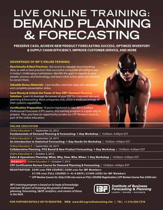
LIVE ONLINE TRAINING:
DEMAND PLANNING
 FORECASTING
PRESERVE CASH, ACHIEVE NEW PRODUCT FORECASTING SUCCESS, OPTIMIZE INVENTORY
 SUPPLY CHAIN EFFICIENCY, IMPROVE CUSTOMER SERVICE, AND MORE
IBF’s training program is based on its body of knowledge
and over 30 years of fostering the growth of demand
planning, forecasting, SOP, analytics, and careers of those
in the field.
For further details or to register: Web: www.ibf.org/onlinetraining.cfm | Tel: +1.516.504.7576
	 Advantages of IBF’s Online Training:
· 	 Benchmarks  Best Practices: Get access to valuable benchmarking
data, as well as best practices that successful companies are using to win
in today’s challenging marketplace. Identify the gaps in regards to your
people, process, and technology, and learn what action plans are required
to correct them.
· 	Valuable Bonus Materials: Case studies, exercises, data-sets, templates,
and complete presentation slides.
· 	Save Money  Unlock the Power of Your ERP / Demand Planning
Solution: Learn to leverage the power of your ERP for improved demand
planning  forecasting. Most companies only utilize a small percentage of
their system’s capabilities.
· 	Certification Preparation: If you’re registered to take IBF’s Certified
Professional Forecaster (CPF) exams, this training program is a great way to
prepare. Plus, you have an opportunity to take our CPF Review Course as
part of the online education.
ONLINE EDUCATION
Online Education 1	 | 	September 22, 2015
	Fundamentals of Demand Planning  Forecasting: 1-Day Workshop | 10:00am–4:00pm EST
Online Education 2	 |	 September 24, 2015
	An Introduction to Statistical Forecasting: 1-Day Hands-On Workshop | 10:00am–4:00pm EST
Online Education 3	 |	 September 30, 2015
	Collaborative Planning, POS Based  New Product Forecasting: 1-Day Workshop | 10:00am–4:00pm EST
Online Education 4 	|	 October 2, 2015
	Sales  Operations Planning: What, Why, How, Who, When: 1-Day Workshop | 10:00am–3:00pm EST
BONUS!** Online Education 5 | October 7, 2015
	CPF Certification Review Course for Demand Planning  Forecasting | 10:00am–4:00pm EST
REGISTRATION: $349 (USD) PER COURSE | $299 (USD) for IBF Members
$1199 (USD) FULL COURSE (1–4) 4 DAYS | $1099 (USD) for IBF Members
CPF Review Course (5), Only $100 (USD) more w/ FULL COURSE Registration | CPF Review Course Fee: $349 (USD)**
compare forecasts with production
line throughput rates to understand
future capacity requirements. For
example, “My forecast is a stable
500 widgets per month, and my
production capacity is capable of
consistently making 600 widgets
per month.” While this example of a
matching process is straightforward,
the important effort in the balancing
process is to project the demand and
supply requirements into the future,
to try to determine the point at
which demand will exceed supply (or
opportunistically find buyers for the
100 extra widgets of your available
supply).
Supply and demand balancing can
be much more complex, particularly
when different products compete for
or share production line time. When
I worked at Snapple, the forecasted
demand for 16-oz. glass bottles of
Snapple Lemon Tea was translated
into a product family called “16ozTea.”
This equated to a supply characteristic
of 0.025 minutes per unit on a 16-oz.
hot-fill production line, one of many
such 16-oz. hot-fill lines. Demand for
all Snapple 16-oz. tea flavor offerings,
including peach, lemon, mint, and half-
and-half, were aggregated into this
16ozTea product family. This product
family view enabled planners to easily
assess the entire capacity network and
to assure our ability to manufacture
product against the forecast over
time. Adding another level of
difficulty to the balancing process
was the inclusion of similar products
competing for the same production
line time. As you might expect, we
had multiple product families such as
16ozJuice and 20ozTea. The 16ozJuice
product family competed directly
with the 16ozTea family for available
production capacity, yet the product
ran slower, was much less seasonal,
and the product had shorter expiry
times, thereby preventing any pre-
building of inventory. Consequently,
the resulting supply and demand
balancing process was much more
intricate than one might expect, with
a lot of conflicting goals—maximize
production utilization, pre-build only
what was needed, manage expiry, use
the least amount of contracted supply,
all while meeting all demand in all time
periods. As I noted, it was challenging
work.
Working through the complexity
of the balancing process yielded a
number of visualization benefits,
including the ability to make decisions
on pre-building inventory in advance
of need (when the production would
not keep up with demand—usually
in the summer months) and when we
needed to add additional capacity
to the supply network via external
contractors. In addition, product
families were also leveraged to
summarize revenue streams. Each
unit of 16ozTea was valued at $0.23,
making it easy to calculate top-line
revenue estimates.
The tangible benefits of this
product family-based supply and
demand balancing act were realized
immediately.Productfamiliesprovided
both a common language and a point
of connection around which personnel
from supply, demand, and finance
could all rally. Forecasters, marketers,
salespeople, and operations personnel
were able to sit around a table and
communicate easily, as the product
family designation became something
of a pivot point for planning purposes.
The results: operations leveraged
working capital much more effectively
and inventory was reduced by
manufacturing products just ahead of
need without extensive pre-building
while also limiting the need for
contracted (expensive) manufacturing
resources.
This use of product families is
commonplace in manufacturing. In
fact, it is a core expectation in SOP;
and on observation, service industries
have a very similar (compared to
manufacturing companies) notion
of product families and supply
and demand balancing. These
organizations seek to balance their
available resources to meet the inflow
of demand for their services, but that
demand needs to be defined. Often,
managers in service industries seek to
control the demand inflow (or outflow)
by matching their estimates of demand
to the capabilities of their ability to
serve. Sometimes they’ll do this to
manage processing costs, other times
to manage the amount of workflow
through available resources, and
other times to orchestrate a desired
outcome. In all of my observations, the
end goal of such processes has always
been to seek balance. Service leaders
achieve this using a matching process
by which they align a service demand
characteristic to a service family;
this translates into service capacity.
It is manufacturing’s product family
concept revisited in the service sector.
It is:
Service Demand ➔  
Service Demand Characteristic ➔  
Service Family ➔ Service Capabilities
To be clear, in all of my observations
of SOP-like planning processes
deployed in service organizations, not
a single one referred to it as a service
family, and no one mapped out a data
translation flow like the one shown
here. This is merely an interpretation
of how they mimicked the concept
of product family in their planning
processes. Almost every observed
	 Copyright © 2015 Journal of Business Forecasting | +1.516.504.7576 | www.ibf.org | All Rights Reserved | Summer 2015	 9
organization had distinct classes of
services provided to different types of
customers, and these different service
classes consumed the organization’s
resources differently. As consumers
of services in everyday life, we see
this dynamic happening all the time,
but we rarely examine the planning
model behind it. Every time we hop
on a plane, we are aware of coach,
business, and first-class seating. These
are different classes of service, each
with somewhat predictable demand
and finite capacity. It is not enough,
however, for airline schedulers to
know the total number of passengers
booked on a plane; they need to
estimate how many in each class or
family of service. From a planning
perspective, the demand for the
different service offerings should be
aligned with the capabilities to deliver
the service. This may seem as simple as
filling seats, but the real opportunity
is knowing how many people want
each class of service so the airline can
adjust the equipment used (either
the number of planes or the seating
configurations for each class) to
match the unconstrained demand
for premium service, and thereby
maximize revenue.
In another seemingly straight­forward
example, consider the challenges of
trying to understand how to staff a loan
processing department in the mortgage
industry. You would need to plan
based on some historical reference for
demand—maybe a monthly tally of all
applicants over the last couple of years.
And in determining service capabilities,
a manager would need to understand
vacations, holidays, and work schedules
of existing employees, and then roughly
the processing time per mortgage, and
estimate—very roughly—the resource
requirements by month. This is an
effective planning process but one likely
to have considerable variances in the
estimates of both supply and demand
because of its relative simplicity.
Of course, this is an example that
screams for more data. A planner would
need to know not only the gross number
of mortgage applicants but also the
number of different types of mortgage
applicants: how many jumbo mortgage
applicants are processed in a month?
How many mid-tier mortgages, condo
or co-op mortgages, refinances, etc., are
normally processed? At most banks, a
potential customer applying for a jumbo
mortgage receives much more personal
attention, more hand-holding—a
premium level of service—compared
with an applicant for a comparatively
smaller mortgage. Applicants for jumbo
mortgages consume more of the service
capacity—the time—of mortgage pro­
cessing agents, they require more follow-
up attention. Thus, the most senior loan
processors are typically engaged to
work with them. Borrowers applying for
jumbo mortgages are treated with more
of a “private banker” service model. It is
worth it because they represent a more
profitable service line. For applicants
seeking mortgages for condos or co-op
apartments, banks must understand the
variouscovenantsandbylawsattachedto
the property, which require a significant
amount of loan processing resources.
Conversely, mid-tier applicants—those
shopping for discounted closing costs
and the lowest interest rates—are
fairly straightforward to manage and
are easy on the resources, but they’re
not as profitable as others. Forecasting
service demand for clients in this
scenario requires enough granularity to
project their loan processing resources.
Jumbo, condo/co-op, and mid-tier
would seem to be perfect descriptors
for these various service families, each
requiring differing amounts of service
time. And being able to project the
average number of requests for each
type of loan application per month
would dramatically help staff the loan
processing department at appropriate
levels. All of these factors are important
elements to consider in achieving a
supply (service) and demand balance.
Two other important characteristics
that are representative of traditional
SOP are product portfolio manage­
ment and strategic alignment. In manu­
facturing terms, product portfolio
managementisthereviewofallproducts
(the portfolio), each month, throughout
their different product life stages. As
consumers of manufactured goods,
we are all aware of products going
through life cycle evolutions. We see
new products on the shelf, we see new
packaging or formulae (“improved”),
and we all have had a favorite product
or two discontinued. In some more
advanced SOP processes, portfolio
management is actually a “review”
meeting by itself, during which all issues
relating to product management are
discussed once a month. In the service
industry this is no different.
According to Dr. Chaman Jain,
a professor at St. John’s University,
“Managing product portfolio and
product mix are equally important
in the service industry, but the way
they view it or call it may be different.
Universities are constantly reviewing
their portfolio of services and eli­
minating the departments/areas that
are least profitable and adding ones
that are most profitable. In recent
years, a number of schools have added
programs of supply chain, predictive
analytics, and big data, to name the few.
They are also changing the service mix
by offering more and more programs
online. Portfolio management in the
service industry represents the shifting
of service offerings toward the direction
of demand. It is not much different than
10	 Copyright © 2015 Journal of Business Forecasting | +1.516.504.7576 | www.ibf.org | All Rights Reserved | Summer 2015
yourgardenvarietyconsumer-packaged
goods company.”
Finally, traditional SOP requires
a monthly revisiting of the strategic
imperativesofthebusiness.Thegoalisto
maintain alignment between demand,
supply, new products, and the strategy
of the organization. In manufacturing,
this may mean focusing limited capacity
on the products with the most strategic
importance or profitability. In the
service sector, I’ve observed a consistent
alignment to the strategic goals of the
organization in concert with a strong
attachment to metrics. Most of the
time, strategic goals were expressed
in terms of how customers were to be
served or markets to be developed.
A mortgage company wanted to be
“easy to do business with” and to “get
to money” quickly. They measure
customer satisfaction from surveys,
but they also measure time spent at
each process step, since customers
consider speed the most important
factor in overall satisfaction. In contrast,
a corrections department considers low
recidivism rates and taxpayer safety, as
measured by survey responses, to be
key elements of their strategic vision.
Such goals have a role in dictating the
type of services provided to inmates in
the correctional system. I have always
believed that SOP is easily replicatable
in the manufacturing sector because the
planning processes are similar in theory,
analytics, and language—despite cross-
industry differences in methods of sales
or modeling of capacity. In as much as
the manufacturing and service sectors
are very different, many of the planning
approaches I observed in service organ­
izations were surprisingly similar to
those used in manufacturing-centered
SOP processes. Some of the examples
that follow are amazing in their depth
and level of integration, tooling, and
metrics,whileotherswerecomparatively
small and narrow, yet no less effective—
limited service planning models that
are mostly simple forecasting. What
gave me great hope of an adaptable
service-industry version of SOP is that
many of the processes overcame the
limitations of extremely divergent views
of supply, demand, and metrics, while
still retaining the core SOP tenets of
collaboration, continuous improvement,
and strategic alignment around a mid-
to long-term plan. You will see plenty of
such similarities as well as some of the
differences outlined in these examples.
Sometimes a single example can save
10,000 words of copy, with that in mind.
I offer six real-life observations.
CONSULTING SOP
EXAMPLES
A decade ago, I spent three years
at a boutique supply chain consulting
company where we had our own,
albeit limited, proxy for an SOP
process. We had a weekly pipeline
call, based on a detailed spreadsheet
of active and potential engagements
(with consulting assignments) and
the expected availability dates of all
the consulting talent. The pipeline call
was essentially a consensus meeting
during which sales and consulting
managers discussed future demand
and consultant availability. They
also sought agreement about the
assignment of consultants to future
engagements. If we needed a specific
skill set to close a deal—someone with
SAP APO expertise, for example, we
knew to project (and source) the talent
we needed as well.
This process was not perfect. It
was not a classic SOP model, and we
certainly did not call it SOP, but it
functioned very similarly. We balanced
supply and demand in both the long
and short terms. We had known orders
(existing ongoing engagements), a
forecast (the sales pipeline), inventory
(the consultants themselves), lead
time (the timing of the availability
of consulting resources), and new
product (new hires). All of these would
go into the aforementioned supply-
and-demand balancing process. Our
goals were to maximize revenue
and minimize consultant downtime
by matching the supply of talent
to the demands of the consulting
engagements. We also sought to direct
our talent strategically by pursuing
engagements that posed the highest
long-term value add.
In support of this process, we
coordinated input from our creative,
marketing, and human resources
groups, and we worked to maintain
alignment on strategic direction. We
created white papers, held seminars,
participated at conferences, leveraged
social media and email blasts, and
hosted webinars to shape demand
toward practice areas we wanted to
emphasize. All of these elements were
discussed as part of the pipeline call.
The process was very SOP-like, sans
the moniker.
SOFTWARE COMPANY
EXAMPLES
I observed a similar demand-
side process when I worked at
two different software companies.
Both companies had sales pipeline
discussions like the one I observed
at the consulting company. They had
numerous prospects representing
future demand and marked each
with a different level of progression
or maturation as it advanced through
the sales cycle. Included in these
pipeline spreadsheets were account-
by-account reviews, with an estimate
of revenue and a probability of closing
	 Copyright © 2015 Journal of Business Forecasting | +1.516.504.7576 | www.ibf.org | All Rights Reserved | Summer 2015	 11
the deal.
Both software companies had
great urgency to predict future service
needs, specifically the availability of
implementation consultants, since the
company’s revenue recognition was
based on fully implemented software.
The pipeline call was a weekly effort
to understand future revenue streams
and to gain alignment between the
sales (demand) and consulting (supply)
organizations, which was necessary
to ensure the timely installation of the
software for clients. When there was
an imbalance between the availability
of internal service talent and the need
to sell the software as well as complete
implementation services, then the
overflow service requirement had to be
outsourced to certified partners.
In these meetings, we tracked
pipeline progress and estimated timing,
closure rates, consultant utilization,
consulting profit as a percentage of
revenue, and even training-class fill
rates. We measured our ability to predict
future demand and the utilization of
resources. And if a prospect needed a
specific feature added to the software,
we engaged RD in a discussion about
projected timing and complexity. In
hindsight, this all seemed to be very
SOP like.There were robust discussions
of demand (projected software sales)
and supply constraints (consultants),
understanding of future revenue
streams,engagementbetweensalesand
RD, and external communication with
key stakeholders (certified partners).
It was not SOP (odd, considering it
was supply chain software), but it was
a detailed, collaborative, short- to mid-
range (1-year+) planning process.
CORRECTIONAL
FACILITIES
Sometimes you get lucky, and
such was the case when I attended
an Institute of Business Forecasting
conference, and randomly walked into
a seminar that described a forecasting
process for a state prison system. In
some states, a prison system can be a
fairly big industry, one that needs to
be managed and balanced with the
needs of public safety in mind. So, how
do you forecast prison usage? It starts
with the court docket. A docket is a
listing of criminal charges against an
individual. In most instances, criminal
cases flow through the justice system
at a rather consistently timed, and
predictable pace, with sentences—in
the event of guilty plea or conviction
fairly easy to estimate. In this example,
projection is based on a rather narrow
set of likely outcomes. A first-time
offender found guilty of first-degree
larceny faces a sentence likely ranging
anywhere from six months to three
years. According to the presenter, the
average court case takes about six
months to be resolved, either by plea
or by trial; and once charges are filed,
conviction rates are very high—more
than 90%—which makes predicting
the timing and sentence duration
of new convicts relatively easy. By
analyzing the historical progression
and timing of yet-to-be-sentenced
offenders as their cases progress
through the criminal justice system,
a planner may reasonably forecast
future demand (prisoners) relative to
the supply (prison capacity) simply by
leveraging the criminal court docket.
Adding a wrinkle to the prison
planning process is that different types
of crime dictate the specific types of
capacity required. Each pre-sentenced
offender is classified in advance.
Violent criminals, for example, warrant
a higher level of security in terms
of capacity (e.g., supermax prisons)
while individuals charged with lesser
offenses, like white-collar crimes or
simple DWIs, require housing in less
secure facilities or perhaps even in
alternative prison programs, such as
home detention or halfway houses.
When capacity in a prison system
reaches its maximum, information
on the prisoner population is passed
to the parole board and to judges.
Capacity actually is part of a judge’s
decision tree when sentencing. It is
also used by parole boards to help
determine whether or not to grant
early parole. There is even a long tail
in prison systems—offenders nearing
the ends of their sentences are often
opportunistically moved to lower-
security facilities or even granted early
release to help free up prison capacity.
The presenter explained how this
specific prison system used an SOP-
like planning process to forecast long-
term capacity requirements while
also balancing supply and demand
with utmost attention on the strategic
imperative of public safety. Dangerous
convicts are held for the duration of
their sentences while lower classification
offenders are released opportunisitically
to make space. The presentation also
helped me to clearly understand pitfalls
unique to poor planning in the service
sector; prison overcrowding.
At the time of presentation, the
actress Lindsey Lohan was released
from custody after serving just a few
hours of a 90-day sentence because
correctional authorities failed to plan
for an adequate number of prison
beds. Needless to say, the presentation
proved to be a fascinating discussion
topic, and in the end it all came down
to how you visualize supply and
demand. I left thinking how clever
the presenter was for creating this
sophisticated SOP-like process with
elegant feedback loops to support the
criminal justice system.
12	 Copyright © 2015 Journal of Business Forecasting | +1.516.504.7576 | www.ibf.org | All Rights Reserved | Summer 2015
SCHOOL SYSTEMS
I have observed the same approach
extended into education—a local
school district that uses statistical
models to predict the need for schools
(opening/closing/mothballing) based
on population statistics. Many districts
are closing or mothballing schools
as children of the baby boomers (the
echo boom) are now getting older and
the student population is temporarily
lower. Keeping schools open and hiring
or laying off teachers are significant
strategic moves that are best made
with a deep, accurate understanding
of the supply and demand balance of
students, teachers, and facilities. In
this model, schools and teachers are
the capacity, while projected student
population represents the demand.
Is this traditional SOP? No. But are
district leaders striving to balance
capacity with future demand? Yes.
In fact, this service-based planning
process is so essential that it is revisited
quarterly, as population estimates
fluctuate. This is clearly a smaller,
limited example of an SOP-like
process, because it has all the critical
elements. Satisfaction is measured in
terms of class sizes, standardized test
scores, and effective use of taxpayer
dollars.
One key factor that points to a
unique urgency for advanced planning
within school systems is the population
of students requiring extra care. This
may range from paraprofessionals
assistingdisabledchildrentoproviding
focused education for learning-
impaired students. There is not one
single type of student, but many. And
these differing types, whether based
on physical or cognitive need, must
be by law served with specific types
of services mandated to educate all
children.
SOP, not exactly. Long range
integrated planning—absolutely.
HEALTH CARE
During an Ops Research class, a
classmate once spoke about a supply
and demand planning process in an
atypical service application. He ran
the radiology unit for a large health
care system in the New York City area.
He was in charge of a wide range of
very expensive equipment, from x-ray
machines to MRI equipment, all of
which needed to be kept fully utilized
to help offset the investment in such
resources.
Obviously patients served by this
equipment arrived with different
levels of prioritization—from critical
care (a head MRI after a car crash) to
less time-critical usage (a knee MRI
prior to meniscus surgery). Scheduling
and allocating the equipment to the
highest-priority needs—as well as
predicting the future utilization and
capital requirements—were all vital
aspects of my classmate’s job.
Like most supply chain managers,
his challenge was to manage the
steady workflow of everyday, low-
priority volume but also to plan in
advance to expedite the unpredictable
demand of critical care patients. He
even employed classic notions from
the manufacturing sector, like buffer
time—periods when the machines
were intentionally planned to be
left idle (i.e., in reserve) even during
times of peak routine demand, to
accommodate the uncertainty of
critical demand—and deferrals,
periods of time when hospital patients
would have radiological procedures
performed overnight, on occasions
when the machines were overbooked
during daylight or evening shifts.
During the daytime and evening, he
would flex-fill this intentional slack
capacity at his discretion, assigning
readily available individuals such as
early outpatient arrivals and hospital
patients so that he was always pushing
any slack time to the back of the shift.
He also devised weekly and
monthly meetings to review forecasts
of loading, segmented by average
demand according to patient type (i.e.,
routine vs. critical care), and medical
department. His consensus group
gathered information from each health
care discipline to get a handle on near-
term needs like scheduled surgeries
and employee work schedules. He
was even able to project long-term
capital expenditure requirements by
determining when utilization was
routinely planned to exceed 80%.
His group used a modified version of
a finite scheduling tool to plan and
balance near- and long-term loading.
This approach was definitely not
full-blown SOP, but my classmate
used many supply chain planning
concepts and tools. He forecasted;
planned using a finite capacity tool;
incorporated effective concepts of
planning for uncertainty; buffered his
inventory of machine time by deferring
lower-priority procedures; pulled
forward demand opportunistically to
fill slack time; developed a balancing
process that matched the resources’
availability to the needs of the patients
over both long- and short-term
horizons; and collected, analyzed, and
incorporated numerous performance
metrics into his overall planning
strategy. He even projected future
needs. He used all of these methods
to gain maximum control over his
service-oriented business operation
because the implications of misusing
the capacity, or underestimating
loading, could result in delivering
potentially life-threatening levels of
	 Copyright © 2015 Journal of Business Forecasting | +1.516.504.7576 | www.ibf.org | All Rights Reserved | Summer 2015	 13
customer service or, alternatively,
wasting incredibly valuable capital if it
were underutilized.
MORTGAGE
INDUSTRY
This final example comes from a
recent discussion with a friend who
runs the mortgage business for a
major bank. He told me of a planning
process similar to SOP that the bank
uses to plan its mortgage business.
He estimates demand for mortgage
applications over both short and
long horizons by looking at historical
ebbs and flows in interest rates,
housing starts, and general economic
bellwethers. Even so, his forecast
is intentionally conservative, to
hedge against downside risk such as
unexpected local economic changes,
like a large layoff by a significant
employer.
The company’s capacity is defined
by its capability to manage customers
(applicants) through the process of
mortgage application, risk assessment,
and closing. The entirety of the
process is measurable in terms of time,
mistakes, and customer satisfaction.
Throughput capacity is a function
of trained, well-qualified back-office
loan processers. The more and better
trained the people are, the greater the
throughput will be.
Thecompanykeepsaclosewatchon
its performance metrics—expected vs.
actual close rates, quality of applicants,
cycle time, step times—that we in the
traditional supply chain world might
view as forecast accuracy, attainment,
or cash-to-cash cycles. The marketing
arm of the bank even tries to shape
demand when mortgage application
rates dip below forecasted thresholds,
soliciting existing mortgage holders
to consider refinancing. The bank has
the advantage of knowing both the
existing and the potential mortgage
rates of its existing customers, and
thus the financial opportunity they’re
being offered.
Monthly planning meetings
focusing on demand and resourcing
are held at a corporate office, while
local offices hold similar meetings that
focus on the front end of the process.
If planners foresee shortfalls in their
projections—gaps in their forecast—
they can respond proactively by
offering teaser rates or discounted
points, typical levers to stimulate or
shape demand for mortgage inquiries.
Again, all of this activity seems a
lot like SOP, including coordination
between sales and marketing and
what most banks call their back-
office or operations group, but no
one calls it SOP. The benefits of
providing exemplary service based
on effective planning, however, help
validate the solid brand identity of this
organization—a bank that is easy to
do business with!
WHAT DO THESE
EXAMPLES
DEMONSTRATE?
From all of these examples, it is
obvious that integrated planning
exists in the service sector, and at
times it is rich, elegant, and robust. It
is not called SOP, nor by any other
related name. It is often shortsighted,
missing some integration points in the
SOP model that would make it better.
My friend in the radiology department,
for example, never shared his results
with his peers. So while he was busy
optimizing his own department, he
may have quite possibly been wreaking
havoc on others. The school system
that I mentioned failed to engage the
local community in its estimates while
pushing for renovations and build outs
of some of its schools. Collaboration
was a point of failure. And although
the corrections department example
was the most complete of all, in terms
of approximating true SOP, its leaders
did not carefully assess the financial
impacts of their decisions, and thus
missed out in meeting their operating
budget.
I did observe similarities in some
planning approaches within the
service sector. The consulting and the
software company examples were very
close in terms of planning tools and
concepts. It was almost as if they were
channeling a professional services
version of service-centered integrated
planning. The correctional and school
system examples were also very similar.
Both had issues relating to capacity
(beds/classrooms and teachers), and
the challenge of effectively classifying
their demand (inmates and students),
an important element in the supply-
and-demand balancing process. This
suggests the potential for a public
services iteration of SOP. I also found
the mortgage company example to
be similar to the operations of an
insurance company I once assessed,
and the radiology equipment example
had remarkably similar parallels to a
transit system with which I am familiar.
I was delighted to observe similarities
within these service segments, the
realization of which led me to believe
that, with the right implementation,
SOP could possibly spread within the
service sector.
When I began seriously considering
the viability of SOP for the service
sector, one of my hypotheses centered
on whether there was potential for
a well-articulated benefit stream.
During my review and assessment of
the various examples detailed here, I
14	 Copyright © 2015 Journal of Business Forecasting | +1.516.504.7576 | www.ibf.org | All Rights Reserved | Summer 2015
recognized tremendous commonality
in the benefit streams of each of
the integrated planning examples I
observed. And although there were no
inventory reductions or improvement
in working capital utilization, the
remaining benefits were mostly
consistent with those typically
resulting from SOP processes
effectively deployed within the
manufacturing sector. These include:
Better Control of the Organization:
The process of actively and frequently
viewing the inflow of demand, as well
as the use of capacity and capabilities,
gives leadership a better feel for the
planning process. The examples that
had an executive review meeting
seemed to have the most overall
satisfaction.
Improvement in Forecasting: Every
organization claimed this benefit and
it seemed to have the most uniform
downstream effect, since it tended
to lead to better utilization of service
capabilities and yield with more
predictable results/revenues. Further,
those organizations that measured
their forecast accuracy seemed to have
the most overall satisfaction with their
planning process.
Demand and Service Shaping:
Several of the organizations were able
to shape their demand stream around
service constraints. The mortgage
company sought to move both
existing customers and new customers
toward refinancing (via incentives)
during the non-peak season, to help
level the load of resources in the loan
processing department. Similarly,
planners in the corrections department
regularly offloaded capacity based on
projected demand. And the radiology
department worked opportunistically
at a tactical/execution level by shift­
ing demand to fill vacancies in the
schedule.
Long-Term Gap Detection/Capital
Outlays: The school system and
corrections department were both
skilled at determining long-term
capital needs and even shorter-term
capacity requirements. The corrections
department had on-site trailers to
use as alternate capacity to provide
housing for lower-level offenders if
they hit overflow. The school system
was excellent at planning in relation
to long-term cyclical trends based
on projected population expansion
and contraction. And the radiological
group assessed its own machine
loading statistics, and looked at
changes in diagnostics methods to
help determine both what type of
equipment to buy, and when, to best
supplement its existing inventory of
x-ray and MRI equipment.
Integrated Service Offering: The
mortgage company was very smart
in terms of integrating services.
Managers required mortgage holders
to have a (free) checking account with
the bank. As an added incentive, they
offered customers a small cash-back
percentage at the end of each year,
based on the value of transactions
processed through their checking
accounts, and thereby raising their
total cash balances. They provided
mortgage holders with premium
discounts on related property
insurance services, and offered highly
competitive rates on other products
such as auto loans.
Measurement Driving Improve­
ment: In their metrics-heavy examples,
the leadership teams felt that regular
and public measurement of results
were a positive force for change and
led to improved revenues, lower costs,
or better utilization.
New Service Creation or Inte­
gration: In many of the commercial
examples, especially those with senior-
level review meetings, managers were
able to readily identify and integrate
new service offerings.The expansion of
the mortgage platform and improved
planning enabled the bank to buy a
failing insurance brokerage. And cross-
marketing efforts between the two
groups helped increase the fortunes
of the insurance company. The
radiological practice partnered with
an outsourced group of radiologists
that afforded the capability to view
scans around the clock and was more
affordable than staffing up by hiring
additional internal resources.
More Consistent Revenue: This was
of great importance to the commercial
service providers, which was a­­ch­
ieved by a better understanding of
demand. Demand shaping based on
the constraints enabled managers
to focus on new—or otherwise
missed—opportunities to serve. The
mortgage company reaped the largest
improvement in benefit streams, while
the software companies and, to a
lesser extent, the consulting company
also saw markedly improved revenues.
A MODEL FOR GOING
FORWARD
Each of the examples described
here provides broad insight into
very different types of demand and
capacity as they are embodied in
different service industries. However,
by looking at the processes used
across all of the organizations, one can
find similarities in the ways supply and
demand are processed and balanced,
as well as how service offerings are
aligned to the strategies of the various
organizations. While no one entity
represents a perfect adaptation of the
SOP conceptual model, compiling a
composite best-of-show, across all of
the examples, suggests there are eight
	 Copyright © 2015 Journal of Business Forecasting | +1.516.504.7576 | www.ibf.org | All Rights Reserved | Summer 2015	 15
core elements that would best enable
SOP for the service sector. These are:
A Notion of Demand: Projections
of the service demanded should occur
formally in a consensus meeting based
on collaboration and inputs from both
internal (statistics and history) and
external sources (such as collaboration
with service partners). All service
estimates should be measured using
a proxy for forecast error (deals
converted, for example, or revenue
projected vs. actuals, etc.). Accurate
projections of service demand will
likely be more difficult to ascertain
than traditional forecasts compiled
in a manufacturing realm. And they
will vary in calculation, in context,
and in the manner by which such
forecasts are presented by company
and industry. Some of these forecasts
will be less like firm projections and
more like an expression of subjective
probabilities. For example, a software
deal with a revenue expectation of
$100,000 and a 90% closure potential
is not as firm as a production forecast
for 100,000 widgets. However, this
inherent uncertainty should not
be an impediment to developing a
forecasting process with an 18- to
24-month horizon. The quality of such
projections should be part of your
discussion in a demand consensus
meeting.
Projected Supply: The service
capabilities/utilization of the organ­
ization should be projected into the
future. Depending on the industry, of
course,thisconceptmaybeexpressedas
the number of available machine hours,
for example, or a projection of future
capabilities, like the number of SAP APO
consultants expected to be available
to work by June of the following year.
Manufacturing companies understand
their process capabilities (We can
make 1,000 widgets per hour). Service
industries need to similarly model such
service constraints around their own
unique demand characteristics. For
example, by analyzing factors like the
average number of critical care patients/
time-in-machine versus the number
of non-critical care patients/time-in-
machine. And as in manufacturing,
service industries should seek to identify
any significant constraints relative to
the throughput of their service delivery,
in an effort to optimize their ability to
serve.
Supply and Demand Balancing:
Projections of demand, expressed in
terms of service families, is matched
against service capability (i.e., I have 100
mortgage applicants estimated for each
of the next 12 months. Can I meet that
demand?), and mismatches are elevated
to a senior-level meeting. As previously
noted, mismatches may actually
indicate opportunities to process more
applicants and identify more available
prison beds than expected, or perhaps
identify other mismatches such as an
MRI machine being overcommitted two
months out. Either way, mismatches
should be escalated to a management
review meeting with a goal of evaluating
the situation—as well as any potential
tradeoffs relative to decision making,
one way or the other—based on the
strategic imperative of the service
entity and understanding of all relevant
financial implications.
New Products: New service offerings
should be part of any discussion
relating to demand. This could be a
new MRI machine, new online classes,
completely new service offerings, or
even an extension of current services.
A bank with a mortgage company
might acquire an insurance company to
develop a suite of services to market to
new homeowners. This suite approach
might (should) change the revenue
potential. It will also likely impact other
operational factors, such as potential
back-office throughput and human
resources requirements. Their impact
on revenue and throughput should be
carefully considered and discussed in
the senior-level discussion.
Strategic Alignment: Strategic goals
and imperatives should drive demand,
supply, or decisions made in relation
to the balancing process. In addition,
metrics should be aligned toward the
achievement of strategic objectives,
which are normally expressed as some
level of quality service expectation.
Deviations and departures from strategy
are topics for discussion at the senior
management review meeting.
Metrics: Measures of the process,
cycle times, costs-to-serve, and utiliza­
tion should be part of a regular review.
Satisfaction—whether it is expressed
in terms of mortgage applicants or the
taxpayer’s sense of security—should be
tracked along the customer experience
curve. Similar to the manufacturing
version of SOP, service-related SOP
should review metrics—particularly any
variations from expected results—at a
senior management review discussion.
Meetings: The planning process
should have a regular rhythm or cycle
to it. Weekly, monthly, or quarterly,
meetings should be part of the process
and modeled in such a way as to foster
collaboration and focus on service-
related demand, capabilities, new
services, and measures. Each of these
steps should incorporate a regular
review component that is designed
to obtain alignment with appropriate
cross-functional teams. As in traditional
SOP, the notion of collaboration—
whether in pursuit of the smartest, or the
most profitable, or the least expensive
solution—is paramount. And a meeting
involving senior leadership should occur
monthly, to inform them of the latest
demand estimates, problems, issues,
16	 Copyright © 2015 Journal of Business Forecasting | +1.516.504.7576 | www.ibf.org | All Rights Reserved | Summer 2015
Demand Planning
 Forecasting
Boot Camp
New York City USA | DECember 16 –18, 2015
CPF Exam Date | December 19, 2015
tel: +1.516.504.7576 | email: info@ibf.org | www.ibf.org /1512.cfm
Institute of Business
Forecasting  Planning
“ This is a great use of money. This is my third
workshop with Dr. Keating, and it gets better every
year. I also continue to learn new things as I grow in
my company. New things I learn here take on new
meaning and become far more applicable.”
	 S. Grabhorn, Director of Mktg Sales /Product Forecasting
	TUPPERWARE
“ I could not possibly offer any suggestions for
improvement. This was such a great workshop!”
	 T. Hatfield, Manager of Planning
	 TOYOTA
super Early Bird
Special!
$1199
* (USD)
WHEN YOU REGISTER
BY SEPT. 30TH
*IBF Members receive an additional $100 off
w/PredictiveAnalyticsandtheUseofBigDataWorkshop
Understanding Forecasting Software and Big Data From the Ground Up
conflicts, capability shortfalls or excess,
metrics, etc.
Financial Assessment: Top-line
revenue and net profit or direct brand
contribution may or may not apply in
the service version of SOP, but certainly
public institutions have budgets and
capital plans. Decisions should be made
based not only on balancing supply
and demand and on aligning with the
strategic imperative, but also on a least-
cost/greatest-profit, and they should
project capital requirements over a two-
to three-year horizon.
SERVICE INTEGRATED
PLANNING PROCESS
MODEL
Long-time SOP practitioners are
keenly aware that sales and operations
planning is not about a specific type
of industry planning; rather, it is
about creating a culture of planning,
measurement, strategic alignment,
and collaboration that permeates an
organization. Knowing this, and after
reviewing all of the prior examples, it is
obvious that the SOP planning model
is extensible and can be adapted for
use in the service sector. To this end,
I propose a process model based on
the common traits culled from these
examples.
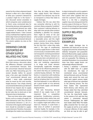
While it might make sense to
borrow from process model diagrams
commonly used to illustrate SOP
implementations in a manufacturing
context—most often a circular or
stair-step model—I think that a simple
linear model serves best as a prototype
to depict an optimal service integrated
planning (SIP) process. You will note
that this model is nearly identical to
the one depicted in Figure 1, which is
the process model for SOP with only
changes in terminology to better aid in
understanding.
As shown in Figure 2, the model
first calls for generating demand
projections or forecasts for baseline
services and any new services. These
are defined as service characterizations
or types. This step is followed by
capacity or capabilities modeling to
represent current estimates of ability
to serve (available capabilities). The
next step is a balancing process by
which managers seek to identify
any inabilities to serve or excess
capabilities by comparing all identified
service-demand characterizations to
the available capabilities. Finally, a
senior management discussion serves
as the monthly process capstone
meeting within which all measures,
issues, gaps to operating plans, and
discussions regarding strategies are
discussed.
A service-based integrated plan­
ning process (SIP) differs from SOP
in a few ways. The service sector is
based on people serving other people.
Decision-making has a different feel
as well. Planning participants must
carefully consider the service objective
or strategy (which should be clearly
spelled out) and always anticipate
how end users may feel about the
service being planned. However, the
mechanics of the process are not
unlike those of a manufacturing-based
SOP process. It is hard not to see
the upside of incorporating an SOP-
like process into the service industry,
or to recognize the great potential
to provide demand and/or revenue
predictability and stabilization.
Although there was not a complete
implementation of SOP in the service
industries surveyed, it’s evident there
are some great integrated planning
practices at work. None of these
matched the high level of process
maturity of the traditional SOP world,
but there is hope.
Documenting examples of these
SOP-like instances—whether as
case studies or in journal articles—
would make significant strides toward
articulating the benefits (and reducing
the risks) of advancing such planning
approaches to a next level of visibility,
awareness, and industry acceptance.
Maybe this article will serve as a spark
for future discussion along these lines.
Call it SOP, SIP, or anything you
want. As the examples in this article
suggest, the basic underlying tenets
and benefits of SOP can be cascaded
into diverse service industries. The
challenge is to find suitable proxies
for evaluating supply and demand, to
align these with your own business
strategies, and then collaborate,
collaborate, collaborate.
—Send Comments to: JBF@ibf.org
.
Figure 2 | Service Integrated Planning Process
Demand Review
(Meeting) Including
New Products
Supply Review
(Meeting)
Supply Demand
Balancing  Exception
Management
Senior Management
Discussion
ISSUES, GAPS, METRICS, FINANCIAL IMPLICATIONS, STRATEGY
ISSUES, GAPS, METRICS, FINANCIAL IMPLICATIONS  SERVICE STRATEGY
Service Demand
Estimation Incl.
New Service Offerings
Service Capacity一
Capabilities Estimation
Service Supply
Demand Balancing
Senior Management
Discussion
18	 Copyright © 2015 Journal of Business Forecasting | +1.516.504.7576 | www.ibf.org | All Rights Reserved | Summer 2015
E x ecu t i v e S ummar y | This column discusses what is commonly known as unconstrained demand, which
represents customer demand devoid of any impacts due to supply limitations. It recommends extending the concept to
focusing on “supply-neutral” demand that also reflects demand devoid of distortions due to supply surpluses and other
supply-related factors. Over time, forecasting demand that is not supply-neutral can “condition” customers to demand
product based on available supply rather than on true demand needs. Several examples of these distortions in real-world
settings are discussed and forecast data cleansing methods are recommended to estimate true demand from the data.
Larry Lapide | Dr. Lapide is a Lecturer at the University of Massachusetts, Boston and an MIT Research
Affiliate. He has extensive experience in industry, consulting, business research, and academia as well as a broad
range of forecasting, planning, and supply chain experiences. He was an industry forecaster for many years, led
supply chain consulting projects for clients across a variety of industries, and has researched supply chain and
forecasting software as an analyst. He is the recipient of the 2012 inaugural Lifetime Achievement in Business
Forecasting  Planning Award from the IBF. He welcomes comments on his columns at llapide@mit.edu.
(This is an ongoing column in the Journal, which is intended to give a brief view on a potential topic of interest to practitioners
of business forecasting. Suggestions on topics that you would like to see covered should be sent via e-mail to llapide@mit.edu.)
Supply-Neutral versus
Unconstrained Demand
By Larry Lapide
I
recently attended an interesting
IBF Boston chapter meeting
hosted by forecast managers at
a Stonyfield Farm Yogurt plant in
New Hampshire. The meeting started
with a plant tour and snacks, and
was followed by a presentation by
its forecasting team. The managers
discussed how forecasting is done
there, a lot of questions were asked,
and discussions ensued to make it a
learning experience for everyone.
After the meeting, I noted to
the leader of the team that I was
impressed by the fact that the
managers had mentioned several
times that they had implemented
forecast methods aimed specifically
at generating “unconstrained” de­
mand forecasts. Most forecasters
recognize that a forecast organization
is ultimately responsible for providing
planners (such as in a Sales and
Operations Planning [SOP] team)
with “unconstrained” forecasts rather
than ones “constrained” in any way by
limited supply. These are essentially
projected business that would be
generated if a company had an infinite
and immediate supply to fill customer
demand—when, where, how, and in
what quantities demanded. Some
forecast organizations, however, don’t
recognize or realize the need, nor do
some take the effort to go far enough
in this regard. Yet from a competitive
perspective, they should, despite the
fact that it is often easier said than
done.
In my Journal of Business Forecasting
(JBF) column, “Forecast Demand or
Shipments?” (Spring 1998), I stated
that “forecasters out there that are
currently using a product’s historical
shipment (or sales) data to forecast
customer demand should take heed.
Use of this data may be dangerous to
your demand forecasts! The primary
	 Copyright © 2015 Journal of Business Forecasting | +1.516.504.7576 | www.ibf.org | All Rights Reserved | Summer 2015	 19
reason for this is that a shipment-based
forecast is often not a clear indicator
of what your customer’s demand for
a product might be in the future.” I
also discussed several anecdotes in
which companies were (unbeknownst
to them) using constrained data for
forecasting, because what appeared to
be unconstrained demand was really
constrained or influenced by other
supply-related factors. I then covered
various methods that might be used to
better align historical shipment data to
better reflect unconstrained demand.
This column updates my view on the
subject.
DEMAND CAN BE
DISTORTED BY
OTHER SUPPLY-
RELATED FACTORS
I recall a comment made by the late
Dick Clark during a discussion about
the difference between constrained
and unconstrained forecasts. Dick,
the consummate industrial forecaster
(who was PG’s forecasting guru for
several decades before he passed
away a few years ago) doubted that
“true” unconstrained demand even
existed. I never really understood
what he meant by this until recently,
largely because I was simply viewing
unconstrained demand as just demand
devoid of any impacts due to supply
shortages—such as distortions caused
by lost sales due to stock-outs or late
shipments due to backorders.
There are times when other supply
factors, such as a surplus of supply, can
affect demand as well. Thus, the term
unconstrained demand is a bit of a
misnomerinthisregard,andtheproper
term should be extended to supply-
neutral demand. Therefore, forecasters
should give the matter more attention
than they do today, because these
other supply factors, that influence
and distort true demand, may not be
as transparent as those that relate to
supply shortages.
I believe that this was what Dick
was somewhat referring to with his
comment. Many companies“condition”
their customers’ ordering behavior to
align with time periods when product
availability is plentiful. For example,
there might be times of the year
when product availability is scarce (at
a reasonable price), and this might
foster customers to avoid buying the
product during these times, despite
the fact that that is when they really
need it. This type of conditioning
caused by supply factors is often done
unconsciously, is not planned for, and is
not transparent. Certainly promotional
activities that influence demand are
consciously done and planned out in
great detail, because the main job of
sales and marketing organizations
is to shape and create demand.
Conceptually, supply-side managers
should not be influencing demand to
the extent that they are conditioning
customer-buying behavior. Yet these
factors, in conjunction with marketing
and sales demand-shaping activities,
lead me to believe that it is no wonder
that Dick believed it is very difficult to
get a good handle on true demand,
devoid of both supply- and demand-
shaping factors.
That said, forecasting demand
devoid of any supply issues is still
important from a competitive
perspective. Conditioning customers
to buy product when, where, how, and
in what quantities it is most convenient
for a supplier might well suffice in the
short-run. However, it could foster a
false sense of comfort in perceived
customer loyalty. For example, in the
short run a customer might be willing
to align its demand to suit its supplier’s
product availability, possibly because
there aren’t other suppliers that can
meet the customer’s needs. However,
there is a risk that a competing
supplier may come along and steal the
business away in the long run. There is
no such thing as long-term guaranteed
business in a competitive free market!
SUPPLY-RELATED
DEMAND
DISTORTION
EXAMPLES
While supply shortages due to
backorders and stock-outs are not easy
to gauge and correct for, at least they are
relatively transparent and purposeful.
Demand influenced by supply surpluses
and other factors is often inconspicuous
and not purposeful. The following six
anecdotal illustrations I’ve encountered
show how these supply factors can
unknowingly influence demand.
1.	 During a workshop I conducted
with the SOP team of a global
tire manufacturer, the topic of
constrained versus unconstrained
demand forecasts came up. The team
leader went around the room and
asked each region’s process leader
what type of forecast was submitted
to the planning process. The first
three leaders that represented
North America, Latin America, and
Europe stated that they submitted
unconstrained demand forecasts.
The last, the Asian-Pacific leader,
to the surprise of all, said that they
submit a constrained demand
forecast. Flabbergasted, the SOP
team leader asked: Why? The leader
glibly answered that “we never get
the supply we ask for, so we submit
a forecast reflective of what supply
we think we may be able to get.”
20	 Copyright © 2015 Journal of Business Forecasting | +1.516.504.7576 | www.ibf.org | All Rights Reserved | Summer 2015
Thus this leader was essentially
distorting true demand and likely
hampering the growth of the region
by submitting demand forecasts that
were not supply-neutral.
2.	 Anewstoremanagerwasresponsible
for ordering inventory for each
week’s promoted sale items. She did
this by reviewing reports showing
each item’s sales performance during
prior promotions. Her predecessor
was conservative in nature, so he
always under-ordered promoted
items to insure none would be left
after the promotion was over. His
store frequently ran out of promoted
items by Friday, despite the fact that
promotions went through Saturday.
Was the new store manager looking
at true demand in reviewing the past
performance of an item? Obviously
not. If she uses this data, her store
will tend to run out early, and leave
little or no inventory for customers
who come in for promoted items on
Saturday. The reports she looks at
represent supply-influenced demand
or demand distorted from the loss of
business from an untold number of
Saturday shoppers—and due to the
conservative nature of the prior store
manager.
3.	 Every August a company shuts down
its plants for summer vacation.
Thus, historically shipments in
August are extremely low, while
shipments in July and September
are extraordinarily high. This is due
to customers ordering earlier than
they wanted, ordering later than they
might like, or just being backordered
because the plants are shut down.
While customers have potentially
gotten used to this over the years, it
is likely that this conditioning might
not bode well for the company in the
long run.
4.	 Corporate buyers for an apparel
retailer always send a mix of sizes to a
store based on the store’s prior sales,
which are similar to the mix of the
average store. The store, however,
is in an ethnic Asian neighborhood
where the population is somewhat
smaller than that of the average store.
Every season the store’s manager has
to drastically mark down the larger
sizes because few people need them.
When she finally marks them down
to below cost, they eventually sell
out. Since all sizes eventually sell,
this indicates to the corporate buyers
that the store’s size mix forecast was
accurate because every size sold
out. The drastic markdowns are not
visible to the corporate buyers, so
they continue to send the store the
same mix of sizes year after year;
and the store manager continues to
mark down the prices of larger sizes
to clear up the surplus stocks. In this
case, the corporate buyers are not
using true demand to allocate sizes.
They are using shipments and sales
that are distorted by a surplus of the
larger sizes that has to be drastically
marked down every year. Obviously,
while there are markdown sales of
the larger sizes in this store, there
really is little true supply-neutral
demand for them.
5.	 A distribution center (DC) in Boston is
frequently out of stock of a particular
item because the manager thinks
the item is too cumbersome, takes
up too much space in his DC, and
consumes too many labor hours to
handle. Whenever a local customer
orders it, the manager often gets the
item shipped to the customer from a
Hartford DC. Corporate distribution
planners that use DC shipments to
determine how much inventory to
deploy, see little being shipped from
Boston; thus they deploy very little
inventory there. Meanwhile, they
deploy a lot in the Hartford DC. It
is no wonder that Boston is always
out of stock and Hartford always has
a surplus. Since Boston customers
typically have to wait longer for their
deliveries coming from Hartford, they
have been conditioned over time to
accept later deliveries, or possibly
gave up and starting ordering from
a competitor. Thus, true demand has
been distorted by the whims of the
Boston DC manager.
6.	 The last situation involved a grocery
storechainthatdidbusinessinPuerto
Rico (PR). Each week, the stores
ordered goods from a warehouse in
Florida where the goods were loaded
in a container for shipment. Often,
after all the ordered goods were
loaded, there would be a lot of extra
space left in the container. So to save
transportation costs, workers filled
in the extra space with paper-goods.
When a store manager in PR got
the extra paper goods and realized
that there was a surplus, he would
conduct a sale to get rid of them.
Over time, the store managers were
running weekly sales—that is, until it
was discovered what the warehouse
workers were doing. In effect, to
reduce transportation costs, the
warehouse workers invariably forced
store managers to heavily discount
paper goods and conditioned
consumers to buy on promotion.This
definitely distorted true demand,
all by creating unnecessary supply
surpluses.
Ineachillustrationabove,shipments
and sales do not reflect supply-neutral
demand for reasons other than just
supply shortages. These include
distortions resulting from supply-
chain manager behaviors/whims,
SOP planner miscommunication, ad
hoc distribution execution, and an
overreliance on shipment/sale data to
22	 Copyright © 2015 Journal of Business Forecasting | +1.516.504.7576 | www.ibf.org | All Rights Reserved | Summer 2015
forecast demand. In all the cases, the
supply-related distortions were not
transparent to demand forecasters. In
addition, it took a lot of investigation
and analysis to assess if true demand
was being distorted by supply, as
well as to identify the specific supply-
related causes.
SUPPLY-NEUTRAL
DEMAND DATA
CLEANSING
A demand forecasting organi­
zation’s primary role is to provide SOP
planners with a demand forecast that
incorporates the impacts of all future
demand-shaping activities planned by
the sales and marketing organizations.
It should not, however, include impacts
due to supply-related factors. This is
what is often termed the unconstrained
demand forecast, though it should be
better extended to a supply-neutral
forecast, devoid of any distortions due
to supply-related factors.
While that sounds reasonable, how
should one develop these forecasts
from historical sales, shipment, and
booking data that include distortions
to true demand caused by both
demand and supply-related factors?
Basically the historical data must first
be cleansed of these distortions before
using it to forecast true demand.
Typically forecasters start with the “de-
promotioning” or demand-cleansing
of the data, which involves sifting
out the effects of sales and marketing
promotional activities aimed at
demand-shaping. Methods for this are
not discussed in this column.
Next the demand-cleansed data
needs to be cleansed of supply-
related distortions to true demand.
While this is normally done today for
supply-shortage distortions to true
demand, this also needs to include the
cleansing-out of other supply-related
distortions. Two general approaches
to cleansing are described below.
The first approach is to try to
capture data at the time of orders that
better reflect supply-neutral demand.
These include:
•	 Capture the date a customer really
wanted the product instead of the
negotiated due-date between the
customer and the company’s sales/
customer service representative.
•	 Capture “lost sales” by keeping track
of orders that were not placed due to
a lack of product availability.
•	 Capture the date of the order, rather
than the date of its shipment.
•	 Capture shipments based on
customer ship-to locations instead
of a company’s ship-from locations.
Ship-to locations would be used
in historical shipments to get
geographical demand profiles. (This
method would have been useful for
the Boston DC example described
above.)
The second approach is to adjust history
to more closely reflect true demand
such as by adjusting shipment and sales
data prior to using it to forecast. Some of
these adjustment methods include:
•	 Capture out-of-stock information
and adjust the shipment/sales data
during out-of-stock periods. For
example, estimate lost sales that
occurred during out-of-stock periods
and add them to shipments in these
periods. (This method would be
useful for the retail store example
described above. That is, estimate
what an item’s promotional sales
would have been on Saturday if the
product were in stock. Then add
the estimate to actual historical
sales from Sunday through Friday.
This would give an estimate of true
demand for the promoted item for a
whole week.)
•	 Capture information on backorders,
as well as order, manufacturing, and
distribution processing delays. Use
the information to adjust historical
order shipment dates.
•	 Capture pricing information and use
it to reduce sales data during periods
where prices were marked down to
“bargain basement prices” to “dump”
unwanted merchandise. (This would
be relevant for the apparel size mix
example described above.)
In addition to these general
approaches, there are also a variety of
ad hoc corrections that will depend
on the nature of the supply-related
distortions. For example, in the case
in which the Asian Pacific SOP leader
was submitting constrained demand
forecasts, this was easily rectified at the
meeting once he realized it should have
been unconstrained demand forecasts.
In the case of the DC workers stuffing
extra paper goods on to unfilled trucks,
this was solved by setting a policy to
stop doing it. A detailed analysis would
have to be conducted in the case of the
Augustplantshutdownstoestimatehow
much business was lost, and how much
product was bought earlier or later than
when customers really wanted it. These
estimates would be used to correct the
supply-distorted shipment data.
In summary, forecasting managers
should evaluate if there are any
demand signals being used that are
distorted by supply-related factors.
Their job is to provide (for example)
SOP planners with a supply-neutral
demand forecast rather than just an
unconstrained one. Failure to do so
might work in the short-term, but does
leave open the risk that a customer
might get tired of being conditioned
by supply-related factors and move on
to a competitor in the long run.
—Send Comments to: IBF@ibf.org
	 Copyright © 2015 Journal of Business Forecasting | +1.516.504.7576 | www.ibf.org | All Rights Reserved | Summer 2015	 23
tel: +1.516.504.7576 | email: info@ibf.org | web: ibf.org /1511.cfm
DoubleTree Hilton Amsterdam | Amsterdam Netherlands
Supply Chain
Forecasting
 P l a n n i n g
Conference
SILVER
PACKAGE
only 1199 EUR |
$1299 (USD)
When you mention this ad
Register
Today!
1 8   –   2 0 N o v e m b e r 2 0 1 5 E U R O P E
w / 1 - D ay P l a n n i n g  F o r e c a s t i n g A n a ly t i c s T u to r i a l
Institute of Business
Forecasting  Planning
Green Valley Ranch Resort, Henderson Nevada USA
Business
Forecasting
 Planning
Academy
( L a s V e g a s A r e a )
August17–18, 2015
•	 	Achieve superior new product
launches and be confident
with your innovation plans
•	 Understand your planning/
forecasting software from the
ground up
•	 Manage big data and leverage
the full potential of demand
signals for better decision
making
•	 Significantly reduce inventory,
improve customer service, and
increase profitability
•	 	Become demand-driven
 learn how to perform
predictive business analytics
•	 Improve SOP  build
credibility for your forecasts
•	 And much more!
SILVER
PACKAGE
only $1299(USD)
When you mention this ad
Register
Today!
tel: +1.516.504.7576 | email: info@ibf.org | web: ibf.org /1508.cfm
Institute of Business
Forecasting  Planning
SOP:
OrganicValley’s Journey
By BethWells
Beth Wells | Ms. Wells is an experienced demand manager with 10 years of experience in forecasting,
economic analysis, and related fields. She has worked at Organic Valley for over seven years in demand planning
and production departments, where her responsibilities have included forecasting, demand planning process
improvement, supply chain analysis, and SOP. Her extensive experience in agriculture and food production
has given her unique insight into the challenges and opportunities of demand planning in these industries. She
holds a Master of Science in Agricultural Economics from Kansas State University, and is a Certified Professional
Forecaster (CPF).
A
s I began to write this article,
a Mark Twain quote came to
mind. It may be an unlikely
pairing, a literary giant and the
discipline of forecasting. However, if
I have learned one thing in my early
career as a forecaster, it is to open
your mind to all the possibilities and
connections, not just the ones that
are obvious. So, as Twain once stated,
“The secret of getting ahead is getting
started.” This can be applied to life in
general, but I would like to take the
liberty of applying it to the discipline
of forecasting. This is the lens I am
choosing to describe a journey we
took at Organic Valley, resulting in a
successful demand planning software
implementation, process maturation,
and lessons learned.
Organic Valley is a farmer-owned
organic cooperative, headquartered
in scenic, southwestern Wisconsin.
In the past 25 years, Organic Valley
has grown from a small, local co­
operative of a dozen members to a
global supplier of organic consumer
packaged goods, and 1,800 farmer
members strong. Incepted as a farmer
marketing cooperative, Organic Valley
is owned by the farmer members
who supply raw materials that are
produced, distributed, and, ultimately,
purchased by consumers in grocery
stores throughout the United States
and in Asia.
In the spring of 2013, Organic
Valley’s Sales Planning-Demand
Management department (a part of
the Sales organization), engaged in a
project to purchase and implement
a new demand planning software.
Our goal in implementing a new
system was to support the needs of
a collaborative, promotionally driven
forecast in a centralized planning
system. The goal of this project was
not only to implement new software,
but to mature planning processes and
forecast performance by improving:
item level accuracy when using top-
down forecast adjustments, access
to statistical analysis, short life cycle
planning, and promotional planning.
E x ecu t i v e S ummar y | Inanefforttosupporttheneedsofacollaborative,promotionallydrivenforecast,Organic
Valley designed and implemented a project to improve the company’s demand planning system and related processes. This
project resulted in a journey that led to successful software implementation, process maturation, and lessons learned. The
experience fostered growth in the business’s understanding of forecasting, and the value it provides.
26	 Copyright © 2015 Journal of Business Forecasting | +1.516.504.7576 | www.ibf.org | All Rights Reserved | Summer 2015
We were also aiming to gain process
efficiencies including improving data
confidence, streamlining data and
system integrations, providing ex­
ception management, and enhancing
data visualization. The technical
challenges we were facing in meeting
this goal included no dedicated
demand planning software, extensive
use of MSExcel for forecasting, and
building a tiered sales and operations
planning process into a functional
demand forecasting software. To
address this goal and the associated
challenges, we identified the fol­
lowing project objectives: increase
process efficiency, increase forecasted
item level accuracy, increase process
flexibility and incorporate advanced
planning functionality.
To achieve our goal, address the
challenges, and fulfill our objectives,
we engaged a cross departmental team
including core team members as well as
business stakeholders. The core team
of seven included a business lead, two
subject matter experts in forecasting
and reporting, IT business intelligence,
integrationanddatabasespecialists,and
aprojectmanager.Theextendedteamof
business stakeholders included subject
matter experts throughout the supply
chain. After several demonstrations of
demand planning software, we selected
a vendor. We worked through planning,
design, and testing. We went live with
the new software in November 2013.
In Twain’s words, this was the “getting
started.” Which leads to the question,
“How have we gotten ahead?”
Primarily, we were successful in
implementing a functional demand
planning software. We were able
to increase efficiency with the im­
plementation of the new software.
One metric we used to measure this
was reducing employee hours spent
on plan maintenance (outside of
forecasting). Prior to implementation
of a dedicated demand planning
software, 30 hours per week were spent
“fixing” the forecast, but not adding
value. We now spend 10 hours per
week on data maintenance, a 67%
reduction in non-value added fore­
casting work. We also increased
flexibility in our data integration
processes. We are now able to pass
a portion of the intended plan
to downstream applications, which
allows us to send updated forecasts on
isolatedproductswith­outcompromising
the integrity of the aggregate demand
plan. It has im­proved our response time
in updating our signal to the production
line. Functionally, a dedicated demand
planning software provided us with the
ability to refine and revise the demand
plan within the software system,
eliminating the extraction of data into
MSExcel for analysis. We now do our
work in the forecasting system instead
of in MSExcel. Our extraction rate went
from 90% pre-implementation to 5%
post-implementation. This has also
improved work productivity and process
efficiency.
Additionally, our process matured
with the implementation of a dedi­
cated system. We successfully de­
signed a tiered planning process.
This process not only included all
elements of demand planning, but
also included our sales and operations
planning (SOP) responsibilities. It
allows us to take a deliberate and
consistent approach to forecasting,
while continuing to serve the need
of our one number SOP culture.
This tiered approach is conducive
to incorporating the art and science
of forecasting. We not only have the
ability to consider judgment and
collaborative inputs, but can build
these inputs on a statistically driven
base. We have a design that allows the
forecaster to build consensus to a one
number SOP. Figure 1 represents the
Detail Stat.
Forecast
Aggregate
Stat. Forecast
Customer
Forecast
Market
Intelligence
New
Business
Total Stat. Base
(user control on
driver 1,2 or 3)
Lost
Business
Demand
Override
Demand Plan
The
Forecaster’s
Plan
Consensus
Override
Consensus
Demand Plan
Influenced by
Sales and Marketing
Judgement
Supply and
Production Capacity
Constrained
SOP
Override
SOP Plan
Figure 1 | Process Design
	 Copyright © 2015 Journal of Business Forecasting | +1.516.504.7576 | www.ibf.org | All Rights Reserved | Summer 2015	 27
process design at a high level.
Finally, we learned lessons along the
way. To reference Twain for a final time,
maybe “the secret of getting ahead is
not only getting started, but learning
along the journey.” Ours was most
certainly a learning journey. The lessons
we learned were not always easy or
profound, but they are important and,
maybe, some benefit can be gained
from sharing them. There is not a magic
number of lessons or an inclusive
list. Instead, they are insights for
consideration and further application.
•	 Strive for forecasting results, not
forecasting rigidity. The most com­
plicated and theoretically correct
approach to forecasting does not
always yield the most beneficial result
to the business.
•	 Build flexibility into your systems and
processes.This will serve you not only
today, but into the future.
•	 Forecast accuracy is important, but
focus on process improvement. It will
get you further.
•	 Strive for positivity and changes that
helpyounotonlygrowasaforecaster,
but also benefit the greater good—
business success.
•	 Before undertaking a major system
implementation, have a clear goal
and purpose. Then, stay committed
to that purpose and advocate for
achieving the goal. Business priorities
change, continue to promote the
value of your project to remain
relevant.
•	 Promote understanding. Translate the
language of forecasting, so that others
can understand what your needs are,
as well as the service you can provide.
•	 Build strong alignment with IT and
other business units. It will help
translatethelanguageandcontribute
to successful implementation as well
as ongoing support.
•	 Use your software implementation
to grow awareness within your
company of what forecasting is and
why it is valuable.
In summary, our goal in im­
plementing a new system was to
support the needs of a collaborative,
promotionally driven forecast in a
centralized planning system. We did
this by implementing a dedicated
demand planning system and through-
process maturation. It has allowed
Organic Valley to move forward in our
understanding of forecasting and the
value it can add to business success.
 ­—Send Comments to: JBF@ibf.org
28	 Copyright © 2015 Journal of Business Forecasting | +1.516.504.7576 | www.ibf.org | All Rights Reserved | Summer 2015
E x ecu t i v e S ummar y | Almost all demand forecasting and planning systems use some form of statistical
forecasting methods that require historical demand data. The closest data to consumer demand is POS and/or syndicated
scanner data. Although, many companies collect and store POS and syndicated scanner data, less than 40% of companies
use POS data for demand forecasting, and less than 10% use syndicated scanner data. Many companies continue to manually
cleanse their historical demand data as a prerequisite for forecasting and planning of their products. Manually cleansing data
is an intensive process that tends to add virtually no value. The primary reason for cleansing data is that traditional demand
forecasting and planning systems are unable to predict sales promotions and correct for outliers. This is a result of the
statistical methods being deployed in the technology—mainly exponential smoothing methods—which are not capable of
measuring and predicting sales promotions or automatically correct for shortages and outliers.
Charles W. Chase, Jr. | Mr. Chase is the Advisory Industry Consultant and Team Lead for the Retail/CPG
Global Practice at SAS Institute, Inc. He is also the principal solutions architect and thought leader for delivering
demand planning and forecasting solutions to improve SAS customers’supply chain efficiencies. Prior to that, he
worked for various companies, including the Mennen Company, Johnson  Johnson, Consumer Products Inc.,
Reckitt Benckiser PLC, Polaroid Corporation, Coca Cola, Wyeth-Ayerst Pharmaceuticals, and Heineken USA. He has
more than 20 years of experience in the consumer packaged goods industry, and is an expert in sales forecasting,
market response modeling, econometrics, and supply chain management. He is the author of the book,
Demand-Driven Forecasting: A Structured Approach to Forecasting, and co-author of Bricks Matter: The Role of Supply
Chains in Building Market-Driven Differentiation. He is also the second recipient of the IBF Lifetime Achievement
Award. (This is an ongoing column in the Journal on innovation in business forecasting.)
CleanseYour Historical
Shipment Data?Why?
By CharlesW. Chase, Jr.
M
ost demand forecasting
and planning initiatives are
abandoned or considered
failures due in part to data quality
challenges. The right data input to
the demand forecasting and planning
processhasseveralimportantdimensions
that need to be considered for success of
any process. Harnessing the right data
for demand forecasting and planning
always appears to be straightforward and
relatively simple. However, bad data, or
use of the wrong data, often is the real
reason behind a demand forecasting and
planning process failure.
	 Copyright © 2015 Journal of Business Forecasting | +1.516.504.7576 | www.ibf.org | All Rights Reserved | Summer 2015	 29
WHAT HISTORICAL
DEMAND DATA
SHOULD COMPANIES
USE?
Almost all demand forecasting
and planning systems use some form
of statistical forecasting methods
that require historical demand data.
In most cases, companies choose to
use product shipment data or sales
orders data to predict the future, as
both are readily available and best
understood by demand planners
who are responsible for the demand
planning process. According to a 2014
Industry Week Research Report, 70%
to 80% of companies still use either
shipment or customer order data for
demand forecasting and planning (see
Figure 1).
Unfortunately, both product ship­
ment data and sales orders contain
several undesirable components such
as incomplete or partial order fills,
delivery delays, and load effects due
to promotions, which represent supply
chaininefficiencies,supplypoliciesthat
do not always reflect true demand, and
sales/marketing strategies designed to
increase consumer demand (e.g., sales
promotions).Shipmentdatarepresents
how operations planning responded
to customer demand, not consumer
demand itself. Demand forecasting
and planning systems must build plans
off a forecast and use shipment data as
a measure of effectiveness in meeting
those plans. Product order data less
any customer returns are the next best
data representing customer product
demand, but not necessarily the best
demand data input for the statistical
forecasting process. The data that
is closest to consumer demand is
POS and/or syndicated scanner data.
Although, many companies collect
and store POS and syndicated scanner
data, less than 40% of companies use
POS data for demand forecasting, and
less than 10% use syndicated scanner
data according to a 2014 Industry
Week Research Report. Everyone
agrees that POS and Syndicated
Scanner data are the closest data to
true consumer demand, yet both these
data streams are among the most
underutilized for demand forecasting
and planning. Furthermore, roughly
70% of companies are using historical
sales (shipments) “adjusted” for trend
and seasonality, and cleansed of
promotions and outliers separating
the historical baseline volume from
Figure 1 | Demand Information Currently Used for Forecasting and Planning
30	 Copyright © 2015 Journal of Business Forecasting | +1.516.504.7576 | www.ibf.org | All Rights Reserved | Summer 2015
the promoted volume.
MANUALLY
CLEANSING
(ADJUSTING)
DEMAND HISTORY
IS A BAD PRACTICE
It is a mystery to me why anyone
would manually cleanse the actual
demand history given all the ad­
vancements in data collection, storage,
processing, and predictive analytics. In
my experience, whenever a company
separated historical baseline volume
from promoted volume, and then
added them back together using
judgment (also known as layering), 1
+ 1 tended to equal 5, instead of 2. The
process of cleansing historical data is a
manual intensive and non-productive
process in my opinion.
The actual history is what happened
unless it was entered into your data
warehouse incorrectly. In fact, in all
my years doing demand forecasting,
the only time historical demand
data were changed (corrected) was
if the data had been entered into the
data warehouse incorrectly, or if the
historical data needed to be restated
due to distribution warehouse
consolidation. Many companies
continue to manually cleanse their
historicaldemanddataasaprerequisite
for forecasting and planning of their
products. It is a manually intensive
process that takes up, in many cases,
80% of a demand planner’s time. I
would only cleanse the data if they
were entered incorrectly into the data
warehouse, or if the organization was
being realigned. There are only a few
reasons to realign historical demand
data. Those reasons are:
•	 Warehouse consolidation and
realignment
•	 Geographic consolidation or
realignment
•	 Acquisitions and realignment
of products
Many companies believe cleansing
historical demand data (shipments) is
a prerequisite when using a statistical
forecasting solution. The true reason
is traditional demand forecasting
and planning solutions are unable
to predict sales promotions or
correct the data automatically for
shortages or outliers. To address this
shortcoming, companies embedded
a cleansing process of adjusting
the demand history for shortages,
outliers, and sales promotional
(incremental) volumes by separating
them into baseline and promoted
volumes. The cleansing process has
become an accepted activity when
a company is using a statistical
forecasting solution to model and
predict future demand. In theory,
manually adjusting (cleansing) demand
history by removing promotional spikes
and outliers improves the forecast
results. Furthermore, it is believed that
cleansing the actual history will produce
a true historical baseline. On the
contrary, it actually makes the forecast
less accurate. This is primarily a result of
the statistical methods being deployed
in the technology—mainly exponential
smoothing methods, which are not
capable of measuring and predicting
sales promotions or automatically
correct for shortages and outliers.
The definition of baseline history
of a product is its normal historical
demand without promotion, external
incentive, or any other abnormal
situation that may be caused by
outliers. An outlier is a too-high or
too-low sales figure in a product’s
history that may occur under special
or abnormal conditions. Promotional
volume is the incremental volume a
company sold due to sales promotions
and trade merchandising. Based on
these definitions, how would anyone
know by how much to raise or lower
the data to create the baseline
volume? Furthermore, are they actually
removing the correct amount of the
sales promotion, or are they removing
seasonality as well?
In many cases sales promotions
are executed around annual seasonal
holidays. This is another reason why
traditional demand forecasting and
planning systems tend to auto select
non-seasonal models because the
seasonality has been removed along
with the sales promotion volume
during the cleansing process. In fact,
they would have been able to use more
sophisticated exponential smoothing
methods like Winters, which is one
of the best methods for measuring
seasonality and predicting it into the
future. Recently, we conducted a test
with a large CPG company where they
ran their normal demand forecasting
process with baseline and promoted
volumes, and a parallel test modeling
all the data holistically (not cleansing
the data). The results were astounding
showing a 5%-10% improvement in
forecast accuracy by modeling the total
un-cleansed demand history. What
we noticed is that the auto select was
choosing only non-seasonal exponential
smoothing methods (moving average)
for the cleansed baseline, rather than the
seasonalexponentialsmoothingmodels.
With the raw historical shipments data
the auto select was selecting Winters
(additive or multiplicative) exponential
smoothing models over 80% of the time.
The result, on average, was a 5%-10%
improvement in forecast accuracy. So, is
cleansing the data and separating it into
baseline and promoted volume really
worth the effort?
	 Copyright © 2015 Journal of Business Forecasting | +1.516.504.7576 | www.ibf.org | All Rights Reserved | Summer 2015	 31
DOES DEMAND
HISTORY REALLY
NEED TO BE
CLEANSED?
Many companies feel data cleansing
and transformation is required to
facilitate the demand forecasting
process.Thismanualprocessisbothtime
consuming and impractical requiring
various rules that use estimates and
experimental tests to assess the results
of cleansed data. The cleansing process
is usually completed for all historical data
during the implementation process, but
the rules developed must be applied in
real time as historical data are generated
over time. Beyond cleansing, a trans­
formation process is often applied to
normalize the input data for units of
measure or changes in product sourcing
locations in the future. Additionally, for
new products that are merely product
line extensions, a transformation process
is used to fabricate historical data that
will provide the necessary inputs for
the statistical forecasting engine. This
new product transformation can now be
done using a new technology capability
called“Product Chaining”and“Life Cycle
Management,” requiring no manual or
rules based transformation.
Data cleansing supposedly re­
moves inaccuracies or noise from
the input to the forecasting system.
In fact, this so-called normalization
tends to create a smoothed baseline
that replicates a moving average.
Operations planning prefers a moving
average forecast for easier planning
and scheduling for manufacturing
and replenishment purposes. Events
such as sales promotions or anomalies
are described as unforecastable, and
normally turned over to the commercial
team to be handled separately using
judgment. By removing and separating
these events during the forecasting
process it is believed to ensure accurate
prediction of the impact of future
occurrences. These events are also used
to assess the lift of a sales promotion
that occurred in the past, helping to
plan for future promotions. Although,
more sophisticated forecasting systems
can detect outliers and corrected for
their impact on the future forecast,
companies still manually remove
(cleanse) them from the historical data
based on rules and past experience. In
my experience, any manual adjustments
to the historical data or to the future
forecast tends to make the forecast less
accurate due to personal bias, whether
intended or non-intended.
Furthermore, exponential smooth­
ing methods can only measure
trend, seasonality, and level (moving
average). As a result, the related sales
promotional data needed to be stripped
away (cleansed) from the demand
history, as well as the demand history
adjusted for shortages and outliers.
After cleansing the demand history the
baseline volume tends to replicate a
predictable smoothed trend and with
little seasonality, which is essentially
simulating a moving average ideal for
non-seasonal exponential smooth­
ing methods. The sales promotion
volume lifts are then layered back
using judgment. Smoothed trend and
seasonal baseline historical data can
be easily forecast with a high degree of
accuracy using exponential smoothing
methods. It’s much more difficult to
forecast the sales promotional lifts that
occur on a regular basis, but may not
always happen in the same time frames,
(i.e., in the same weeks or month into the
future) as they did in the past. Also, the
durations for such sales promotions may
change, or can be different (i.e., 4 weeks,
6 weeks, and overlapping). Exponential
smoothing methods are traditionally
deployed in over 90% of demand
forecasting and planning solutions
makingitdifficulttomeasureandpredict
sales promotions, or adjust for shortages
and outliers. Once the demand history is
cleansed, the demand planner forecasts
the baseline history (also known as the
baseline forecast). Upon completion
of the baseline forecast, the demand
planner manually layers in the future
sales promotion volumes created by
the commercial teams (sales/marketing)
using judgment, as well as other events
to the baseline forecast to create the
final demand forecast.
Today, new demand forecasting
and planning solutions can holistically
model trend, seasonality, sales
promotions, price, and other related
factors that influence demand using
predictive analytics. In addition, these
same models can automatically correct
for shortages and outliers without
cleansing the actual demand history.
Methods such as ARIMA, ARIMAX, and
dynamic regression models can be
deployed up and down a company’s
business hierarchy to holistically model
trend, seasonality, sales promotion lifts,
price, in-store merchandizing, economic
factors, and more. Intervention variables
(dummy variables) can be used to
automatically adjust the demand history
for shortages and outliers. There is no
longer the need to cleanse the demand
history for shortages, outliers, and sales
promotional spikes. In fact, these same
predictive methods can measure the
impact of sales promotions—calculate
the lift volumes and predict the future
lifts in different time intervals based
on marketing event calendars. In
addition, the commercial teams (sales
and marketing) can spend more time
running “What If” scenarios with
precision, rather than judgmentally
layering back the sales promotional
32	 Copyright © 2015 Journal of Business Forecasting | +1.516.504.7576 | www.ibf.org | All Rights Reserved | Summer 2015
volumes to the baseline volume.
Figure 2 illustrates how a holistic
model captures the baseline (trend
and seasonality) along with sales
promotions while correcting for
shortages and outliers.
HOW MUCH DATA
SHOULD BE USED?
An accurate statistically generated
forecast has several elements in­
cluding trend, seasonality, holidays,
sales promotions, marketing events,
and other related causal factors. There
must be sufficient demand history in
order to statistically model the patterns
associated with these elements to
produce an accurate forecast for future
periods. In most cases, this means a
minimumofthreeyearsofhistoricaldata,
and ideally three or more would be best.
Just to capture the effects of seasonality
there must be three years of historical
demand whether weekly or monthly.
Most demand forecasting and planning
systems use monthly summaries of
Figure 2 | Holistic Model Using an ARIMAX Model
product demand separated either by the
manufacturing source or the distribution
point. In other words, the data must also
reflect the business hierarchy with the
same periodicity (historical time horizon)
including geography, market, channel,
brand, product group, product, SKU, UPC,
and customer/demand point. Although
less data can be utilized in one to two
years, the results may not completely
reflect the true nature of demand,
particularly in regards to seasonality,
holidays, and promotional effects.
SUMMARY
In 2015, demand planners are
still spending over 80% of their time
cleansing, managing, and disseminated
data and information across the
organization, rather than using the
data and information to improve
forecast accuracy. They are merely
managers of data and information.
As “Big” data continues to grow in
volume, velocity, and variability, and,
with more pressure to drive revenue
growth, demand planners will be asked
to not only improve forecast accuracy,
but also find new insights that are
actionable to proactively drive profit.
As such, companies need to invest in
new technology, predictive analytics,
and skills. Demand planners will need
to transition from managers of data
and information to demand analysts
with a focus on predictive analytics
driving revenue growth and profitability.
Recent research indicates that improved
forecast accuracy can add as much as
ten percent to revenue and profitability.
“Manually cleansing historical demand?
Let’s make that history. ”
—Send Comments to: JBF@ibf.org
REFERENCES
1. 	2014 Industry Week. SAS Demand-
Driven Forecasting and Planning Report,
pp. 1-14.
2.	Chase Jr., Charles W. Demand-Driven
Forecasting: A Structured Approach to
Forecasting. New York: Wiley  Sons, 2nd
Edition. 2013.
	 Copyright © 2015 Journal of Business Forecasting | +1.516.504.7576 | www.ibf.org | All Rights Reserved | Summer 2015	 33
worldwide merchandize exports, clearly point out an
undergoing global slowdown contradicting the media-
created myth of transitory snowstorms in New England as
the cause of an economic downswing in the United States
in the first quarter of this year. In March of this year, global
exports, on a year-to-year basis, declined by 12.4%, the
sixth consecutive monthly decline in a row following an
expansion since October 2014. On a quarterly basis, in the
first quarter of 2015 global exports dropped 10.2% from a
year ago to $3.7 trillion, following a 2.6% decline in the last
quarter of 2014. A major trigger for such dramatic changes
in each county’s business cycle has been the “burst” of the
oil-price bubble coupled with currency realignments from
INTERNATIONAL
ECONOMIC
OUTLOOK
Dr. Simos is Director of Forecasting and Predictive Analytics at e-forecasting.com, a division of Infometrica’s Data Center, 65
Newmarket Road, Durham, NH 03824, U.S.A. and professor of economics at Paul College, University of New Hampshire,
www.infometrica.com, eosimos@e-forecasting.com. This report does not purport to be a complete description of global
economic conditions and financial markets. Neither the Journal nor Infometrica, Inc. guarantee the accuracy of the projections,
nor do they warrant in any way that the use of information or data appearing herein will enhance operational or investment
performance of individuals or companies who use it. The views presented here are those of the author, and in no way represent
the views, analysis, or models of Infometrica, Inc. and any organization that the author may be associated with.
In the first quarter of 2015, economic growth in the major
countries, which maintain quarterly national accounts,
was weaker than in any quarter since the end of the great
recession. Revised and more complete estimates of real GDP
show negative growth rates in the United States and Canada
and anemic growth rates in most of the other countries.
In the worldwide business cycle, the group of the English-
speaking countries has led historically global economic
activity. Monthly predictive analytics signal an underlying
weakness for several months in the English-speaking
countries, which have posted negative or steadily declining
growth rates in their leading indicators.
Globally, trade predictive analytics, which summarize
I. Global Assessment and Outlook
Will High Risk
Events Trigger a
Recession?
By Evangelos Otto Simos, Ph.D.
34	 Copyright © 2015 Journal of Business Forecasting | +1.516.504.7576 | www.ibf.org | All Rights Reserved | Summer 2015
The baseline forecast incorporates major findings of the
World Economic Survey conducted in the second quarter of
2015 by the Center for Economic Studies (CES) at the Ludwig
Maximilian University and the German Ifo Institute. About
1,100 executives from 115 countries have indicated that the
world’s economic climate edged up for a second quarter in
a row after “tumbling” in the last quarter of 2014. The major
findings of the second quarter’s survey are as follows:
•	 Worldwide, executives evaluated the current economic
situation, second quarter of 2015, to be slightly above
satisfactory levels, led by an improvement in consumer
expenditures while capital expenditures remain below
satisfactory levels. They found economic activity in their
countries in the second quarter of 2015 to be better than
in the second quarter of 2014. Most important, regarding
the future, executives are optimistic expecting economic
conditions in the last two quarters of 2015 to be above
those prevailing in the second quarter of this year.
•	 On a regional basis, North American executives assessed
the current economic situation to be above satisfactory
levels and better than a year ago. Looking forward,
business experts from the United States and Canada expect
economic conditions to get better in the next six months. In
Asia, executives appraised the current economic situation
to be below satisfactory levels and worse than a year ago;
they were optimistic about the future, expecting economic
activity in the next six months to be better than in the
second quarter of 2015. In Western Europe, executives’
appraisals of current conditions were above satisfactory
levels and above economic levels that they experienced
in the second quarter of 2014; expectations of European
business executives for the rest of 2015 indicate a level of
optimism supporting the view that Europe will remain on it
recovery path.
•	 With respect to prices, survey participants expect average
worldwide inflation over the next two quarters to be above
current levels.
•	 Looking at world trade, the business executives’ combined
expectations predict the volume of both exports and
imports to improve modestly in the last two quarters of this
year compared to present trade flows in the second quarter
of 2015.
•	 Regarding financial markets, survey participants expect
short-term rates to slightly edge up over the next two
quarters; long-term interest rates are expected to rise from
current levels.
Using the “soft data” findings of the World Economic
Survey, a 115-country composite global predictive analytic is
constructed by e-forecasting.com to evaluate and forecast
the short-term worldwide business cycle. A reading of 50,
II. Short-Term Indicators and Forecasts
the strengthening of the U.S. dollar as well as a slowdown in
the growth in emerging economies.
In addition to geopolitical risks related to the Middle
East and Eastern Europe, there is high probability of one
or more policy-created bubbles bursting this year. A hard
landing in China from housing prices and/or stock market
corrections; disintegration of the Euro Area; high debt-
to-income ratios—both private and public—in several
countries; and the timing of an exit from an ill-conceived
and permanent-perceived monetary policy of zero interest
rates in the United States. Any of these events may trigger
a significant correction in stock markets leading to another
major recession with no tools left for economic policy.
Assigning a 40% probability that any of these events will
come suddenly into play this year and thus the risks will be
gradually and orderly managed over the long run, we consider
the current global economic slowdown to be a “soft patch,”
which will maintain over the forecast horizon the ongoing
moderatesix-year-oldpathofrecovery.Undertheseconditions,
the baseline forecast predicts worldwide output to increase by
just 2.7% in 2015, which is 0.5% below the moderate growth
of 3.3% in 2014. Under this scenario, global economic growth
is expected to stay on the existing trajectory for the rest of
the decade with low investment, slowing productivity, lack of
job creation, declining real wages, and halving of the growth
in international trade from its established long-term trend for
decades before the great recession.
In the inflation front, the effect of lower energy prices
has evaporated as oil prices quickly ended their free
fall. It is expected over the forecast horizon oil prices will
fluctuate around one-half of their latest peak. Inflationary
expectations have begun to build up again driven by rising
labor costs from social pressures in a climate of declining or
stalling productivity.
	 Copyright © 2015 Journal of Business Forecasting | +1.516.504.7576 | www.ibf.org | All Rights Reserved | Summer 2015	 35
Table 1 | Global Economic Growth and Inflation
REGION
Market Size
2014 GDP
$PPP Billion
Economic Growth
percent change in real GDP
Inflation
percent change in consumer prices
2014 2015 2016 2017 2014 2015 2016 2017
WORLD 98,320 3.3 2.7 3.2 3.4 3.5 3.9 4.2 3.9
EUROPEAN UNION (28) 18,526 1.4 1.6 1.8 1.9 0.5 0.5 1.2 1.5
	Euro Area (19) 13,155 0.9 1.4 1.6 1.6 0.4 0.4 1.0 1.2
	Austria 395 0.3 0.8 1.3 1.4 1.5 1.0 1.5 1.6
	Belgium 481 1.0 0.9 1.5 1.5 0.5 0.4 0.9 1.1
	Cyprus 27 -2.3 -0.6 1.2 2.0 -0.3 0.2 0.9 1.3
	Estonia 36 2.1 2.2 2.7 3.4 0.5 1.2 1.7 2.0
	Finland 221 -0.1 0.2 1.0 1.5 1.2 0.7 1.6 1.7
	France 2,581 0.4 0.9 1.4 1.7 0.6 0.4 0.8 1.1
	Germany 3,722 1.6 1.7 1.8 1.5 0.8 0.5 1.3 1.5
	Greece 284 0.8 0.4 2.0 3.2 -1.4 -0.9 0.3 0.8
	Ireland 227 4.8 3.1 3.0 2.8 0.3 0.5 1.5 1.6
	Italy 2,128 -0.4 0.6 0.9 1.1 0.2 0.4 0.8 1.0
	 Latvia 48 2.4 2.2 2.8 3.7 0.7 0.9 1.7 2.3
	 Lithuania 80 2.9 2.6 3.0 3.4 0.2 0.7 2.0 2.2
	Luxembourg 51 3.1 2.6 2.5 2.3 0.7 1.1 1.6 1.7
	Malta 14 3.5 3.1 2.8 2.6 0.8 1.2 1.4 1.6
	Netherlands 799 0.9 1.4 1.6 1.7 0.3 0.4 0.9 1.1
	Portugal 280 0.9 1.4 1.7 1.4 -0.2 0.4 1.3 1.5
	 Slovak Republic 153 2.4 2.6 3.0 3.2 -0.1 0.6 1.4 1.7
	 Slovenia 61 2.6 2.0 1.9 1.8 0.2 0.9 0.7 1.5
	Spain 1,566 1.4 2.3 1.9 1.8 -0.2 0.2 0.7 0.8
	 Non-Euro Area (9) 5,372 2.7 2.2 2.3 2.6 0.7 0.7 1.7 2.0
	 Bulgaria 129 1.7 0.9 1.1 1.8 -1.6 0.4 0.6 1.2
	Croatia 88 -0.4 0.1 0.8 1.4 -0.2 0.2 0.9 1.4
	 Czech Republic 315 2.0 2.2 2.4 2.5 0.4 0.4 1.3 2.0
	Denmark 250 1.1 1.5 1.9 2.1 0.6 0.9 1.6 2.0
	Hungary 246 3.6 2.4 2.1 2.2 -0.3 1.0 2.3 2.9
	Poland 954 3.4 3.0 3.2 3.6 0.0 0.3 1.2 1.7
	 Romania 393 2.8 2.5 3.0 3.4 1.1 0.9 2.4 2.5
	Sweden 448 2.1 2.2 2.5 2.7 -0.2 1.1 1.5 1.9
	 United Kingdom 2,549 2.8 2.1 2.0 2.2 1.5 0.8 1.9 2.0
OTHER EUROPE 6,261 0.9 -1.0 1.7 2.0 7.4 11.8 7.8 5.7
Norway 345 2.2 0.8 1.5 1.8 2.0 1.8 2.3 2.3
Russia 3,565 0.6 -2.5 1.3 1.4 7.8 15.0 9.8 6.5
Switzerland 473 2.0 0.9 1.4 1.5 0.0 -0.5 -0.4 0.4
Turkey 1,508 2.9 2.4 3.0 3.6 8.9 7.0 6.5 6.0
Ukraine 371 -6.8 -6.0 1.0 2.0 12.1 28.0 10.6 8.0
NORTH AMERICA 21,151 2.4 1.7 2.1 2.3 1.9 1.5 2.3 3.1
Canada 1,592 2.5 1.4 2.0 2.0 1.9 1.2 2.2 2.5
Mexico 2,141 2.1 2.2 2.7 3.1 4.0 3.0 3.5 4.0
United States 17,419 2.4 1.7 2.0 2.2 1.6 1.4 2.2 3.0
SOUTH AMERICA 6,241 0.6 -0.6 1.2 2.1 12.8 18.9 17.8 13.6
Argentina 948 0.5 -0.9 -0.5 0.3 21.4 17.0 30.0 23.6
Brazil 3,264 0.1 -1.5 1.3 2.3 6.3 8.5 6.2 5.0
Chile 409 1.8 2.8 2.7 3.6 4.4 3.6 3.2 3.0
Colombia 640 4.6 2.1 3.7 4.0 2.9 4.5 3.8 3.9
Peru 371 2.4 2.8 3.5 5.5 3.2 3.2 3.0 2.5
Uruguay 70 3.3 2.6 2.8 3.0 8.9 8.0 7.5 7.1
Venezuela 539 -3.9 -4.0 -3.2 -2.5 62.2 135.0 120.0 90.0
ASIA  PACIFIC INDUSTRIAL 7,784 1.2 1.4 1.8 2.0 2.3 1.3 2.0 2.1
Australia 1,095 2.7 2.1 2.6 3.1 2.5 2.1 3.0 2.4
Japan 4,751 -0.1 0.7 1.1 1.0 2.7 1.1 1.5 1.8
Korea 1,779 3.3 2.8 3.0 3.7 1.3 1.5 2.5 3.0
New Zealand 159 3.2 2.6 2.9 2.5 1.2 1.5 2.1 2.0
EMERGING ASIA 32,900 6.5 5.7 5.6 5.5 3.5 3.1 3.8 3.7
China 17,617 7.4 6.0 5.8 5.5 2.0 1.8 3.0 2.9
Hong Kong 398 2.3 2.1 2.7 3.4 4.4 3.6 4.0 3.5
India 7,376 7.2 6.5 6.2 6.0 6.0 5.4 5.7 5.6
Indonesia 2,676 5.0 4.8 5.2 5.8 6.4 6.6 5.0 4.8
Malaysia 746 6.0 4.5 4.9 5.0 3.1 2.6 2.7 2.5
Pakistan 882 4.1 4.0 4.1 4.8 8.6 5.1 5.0 5.0
Philippines 692 6.1 5.8 6.1 6.0 4.2 2.6 3.4 3.8
Singapore 453 2.9 2.4 2.7 3.2 1.0 0.5 2.0 1.9
Taiwan 1,075 3.7 3.3 3.6 4.1 1.2 0.8 1.8 1.5
Thailand 986 0.7 3.0 3.5 4.1 1.9 1.3 2.4 2.2
MIDDLE EAST  AFRICA 5,456 2.5 1.9 2.1 2.6 7.4 8.2 7.8 7.6
Egypt 943 2.2 2.9 3.2 4.5 10.1 12.0 9.8 9.7
Iran 1,334 3.0 1.0 1.3 1.5 15.5 18.0 17.0 17.0
Israel 268 2.8 3.0 3.1 3.0 0.5 0.5 1.5 2.1
Saudi Arabia 1,606 3.6 2.4 2.6 3.1 2.7 3.0 3.2 2.8
South Africa 705 1.5 1.7 2.0 2.4 6.1 5.0 6.1 5.5
United Arab Emirates 600 3.6 2.8 3.0 3.4 2.3 2.4 2.3 2.5
The 63 countries in this table account for 92% of world’s estimated GDP expressed in PPPs in 2014. 	
Source: www.e-forecasting.com
36	 Copyright © 2015 Journal of Business Forecasting | +1.516.504.7576 | www.ibf.org | All Rights Reserved | Summer 2015
the flatline, is used as reference in evaluating the wave of
alternating booms and busts that mark the global economy.
In the second quarter of 2015, our global business predictive
analytic registered a reading of 56.7 from 54.4 in the first
quarter, which indicates that worldwide economic activity,
is back on its recovery path.
e-forecasting.com’s global business predictive analytic
of business activity tracks quarterly and in a timely way
economic conditions around the world. Its historical
behavior is consistent with the index of industrial production
for a group of 23 advanced economies, so-called industrial
countries, constructed by “hard data”and maintained by the
International Monetary Fund (IMF). However, IMF’s industrial
production index lags our predictive analytic diffusion
indicator in terms of timeliness by one to two quarters. The
e-forecasting.com global business activity index is a “real
time”predictive analytic providing readings at the end of the
last month of the reference quarter as well as predictions for
two quarters ahead.
Historically, changes in our global activity index mirror
the year-to-year growth rate of worldwide industrial
production (see Chart 1). In the fourth quarter of 2014, the
last available reading of the production index (hard data),
industrial production in the advanced economies rose after
three consecutive quarterly declines in 2014. Based on the
real time behavior of our business predictive analytic, year-
to-year growth in industrial activity in the world’s advanced
economies is estimated to have been almost nil in the first
quarter of 2015 and moderately positive in the second
quarter.
By modeling business executives’ two-quarter-ahead
expectations into a dynamic high frequency forecast, our
global predictive analytic anticipates a recovery in the
growth of global business activity in 2015. Looking forward,
based on the path of the global business predictive analytic,
industrial production in the advanced economies is forecast
to continue advancing in the last two quarters of 2015.
Our composite predictive analytic of global business
activity also serves as a gauge of worldwide demand and,
consequently, its change from a year ago mirrors the year-
to-year growth rate in the demand for internationally traded
goods. Derived from the opinions of about 1,100 business
experts from 115 countries, e-forecasting.com’s predictive
analytic of global business activity has shown a strong
performance record in tracking the volume of international
trade, measured by the dollar value of global exports
adjusted for price changes (see Chart 2).
In 2014, the volume of international trade, measured by
real merchandise exports, averaged 2.6%. The predictive
power of our global business activity index suggests that
the volume of world trade has stalled in the first quarter
of 2015 and has modestly increased in the second quarter.
Based on the executives’ anticipations on the future path of
global business activity, the volume of international trade
is forecast to continue increasing in the last two quarters of
this year.
III. REGIONAL CONTRIBUTIONS TO GLOBAL GROWTH
In our baseline annual forecast, global output—a
worldwide composite of 60 countries that account for 92%
of the world’s GDP using as weights each country’s relative
GDP converted to international dollars at purchasing-power-
parity (PPP)—is estimated to have advanced by 3.3% in 2014
and is expected to grow by 2.7% in 2015. Growth in global
output is forecast to slightly accelerate to 3.2% in 2016 and
3.4% in 2017.
Given the relative economic size and expected output
growth in each of the major regional blocs, the contribution
of each region to global economic growth is computed so
that we may identify the distribution of worldwide growth
and, consequently, the allocation of global demand among
geographic areas along with its changing pattern over the
forecast horizon.
The baseline forecast calls for output in the countries of
the North American region (NAFTA) to advance by 1.7% in
2015 and 2.1% in 2016. Thus, NAFTA will contribute 13% in
2015 and 14% in 2016 to the growth of global demand as
measured by worldwide GDP.
In the Euro Area, the combined real GDP of the 19
members of the European Union (EU) that use the euro
as common currency, GDP is forecast to edge up 1.4%
in 2015 and increase 1.6% in 2016. As a result, the Euro
Area will be a positive contributor to global growth
providing 7% in both 2015 and 2016 to the growth of
worldwide demand.
In the Emerging Asia region—which includes the two
38	 Copyright © 2015 Journal of Business Forecasting | +1.516.504.7576 | www.ibf.org | All Rights Reserved | Summer 2015
Table 2 | Contribution of Regions to Global Growth
Region
Percentage Points Contribution Relative Contribution, Percent
2014 2015 2016 2017 2014 2015 2016 2017
EUROPEAN UNION (EU27) 0.28 0.30 0.34 0.35 8.3 11.0 10.5 10.4
Euro Area (euro17) 0.13 0.18 0.21 0.21 3.8 6.6 6.6 6.2
Non-Euro Members (10) 0.15 0.12 0.13 0.14 4.5 4.4 3.9 4.1
OTHER EUROPE 0.06 -0.06 0.11 0.12 1.8 -2.3 3.3 3.6
NORTH AMERICA 0.51 0.37 0.44 0.49 15.5 13.5 14.0 14.4
United States 0.43 0.30 0.35 0.39 12.9 11.0 11.1 11.5
SOUTH AMERICA 0.04 -0.04 0.07 0.13 1.1 -1.4 2.3 3.8
ASIA  PACIFIC INDUSTRIAL 0.09 0.11 0.14 0.15 2.8 4.1 4.4 4.5
EMERGING ASIA 2.12 1.89 1.92 1.94 64.0 68.9 60.3 57.7
China  India 1.79 1.56 1.56 1.53 53.8 56.8 48.9 45.6
MIDDLE EAST  AFRICA 0.14 0.10 0.12 0.14 4.3 3.8 3.6 4.2
WORLD GROWTH1
3.3 2.7 3.2 3.4 100.0 100.0 100.0 100.0
1
Sum of Regional Contributions Source: www.e-forecasting.com
most populous and fastest growing countries, China and
India—growth in output is forecast to average 5.7% in 2015
and 5.6% in 2016, faster than any other economic bloc.
Accordingly, the Emerging Asia region will contribute 69%
in 2015 and 60% in 2016 to the growth of global GDP.
In the industrial bloc of Asia and Pacific region—which
includes Japan, Korea, Australia, and New Zealand—growth
in output is forecast to average 1.4% in 2015 and 1.8% in
2016. Consequently, the Asia and Pacific industrial club will
contribute about 4% in both 2015 and 2016 to the growth of
global demand as measured by worldwide GDP.
Real GDP in the major countries in South America is
forecast to decline by 0.6% in 2015 and then increase by
1.2% in 2016. As a result, South America is expected to
have a 2% contribution to the growth of gobal demand
in 2016. 	 —Send Comments to: JBF@ibf.org
Powerful,Affordable Forecasting
and Forecast Management
• Proven forecasting methods
• Flexible forecast adjustments
• Multiple conversions  hierarchies
• Flexible reporting options
• Accuracy tracking
• Exception reporting
• Team forecasting
• Customizable forecast worksheets
• And so much more!
www.forecastpro.com
See for yourself! Visit our site to
✔watch quick tour ✔download demo ✔schedule WebEx demo
Forecast Pro TRAC includes:
	 Copyright © 2015 Journal of Business Forecasting | +1.516.504.7576 | www.ibf.org | All Rights Reserved | Summer 2015	 39
Dr. Onvural is an Associate Professor of Economics and Finance at Pfeiffer University’s School of Business, teaching online and
face-to-face Business Economics, Health Economics, Health Care Financial Management, and Managerial Finance courses to
the MBA and MHA students.
C
onsensus expects the country’s GDP growth rate to
remain in the neighborhood of 2.3% well into the second
quarter of 2016 even though real GDP declined (now at
a negative 0.2%) in the first quarter of 2015. Specifically, Rajeev
Dhawan of the Economic Forecasting Center at Georgia State
University’s J. Mack Robinson College of Business expects the
U.S. economy to bounce back in second quarter because of
WOW.“The three components of WOW shaved off close to 2.5%
ofU.S. growth in thefirstquarter,”Dhawansaid.(WOWstandsfor
weather, oil, and the world economy.) The GDP report showed
clear damage from these three factors.
Dhawan mentioned further in his report that unusually cold
weather in the Northeast during the first quarter resulted in a
reduction of nondurable consumption goods (to a negative
0.3%), spending on utilities (heating) increased, and overall
gasoline savings were wiped away. “We’ve almost reached
the bottom, with oil rig counts having dropped sharply with
only a little bit to go,” wrote Dhawan.“ But prices will not reach
the heights of $120 a barrel anytime soon. I expect oil to start
creeping up to $70/barrel by year’s end and stay in that range
for the coming year,”he added. Finally, the world economy factor
influenced the real GDP due to the dragging recovery of China
(now at 7%, down from double digits) and the European Central
Bank’s bond-buying program. Chinese economy’s slow-paced
recovery affects the emerging markets because of supply chain
connections. Eurozone’s challenge is related to a potential Greek
rescue operation and the trillion-dollar liquidity injection (bond
buying program) by the European Central Bank, which results in
negative government bond yields. Consequently, these factors
led to a decline in exports (now at a 2.3% decline).
The U.S. Economy to
Bounce Back
in Second Quarter
By Nur Onvural, Ph.D.
Participants | Beacon Economics = Los Angeles, California; Conf. Board = Conference Board, New York, New York; Fannie Mae = Fannie Mae,
Washington, D.C.; IHS = IHS Global Insight, Eddystone, Pennsylvania; GSU – EFC = Georgia State University, Economic Forecasting Center, Atlanta,
Georgia; Moody’s Economy = Moody’s Economy.com, Westchester, Pennsylvania; Mortgage = Mortgage Bankers Association, Washington, D.C.; NAM
= National Association of Manufacturers, Washington, D.C.; Northern Tr = Northern Trust Company, Chicago, Illinois; Perryman Gp = The Perryman
Group, Waco, Texas; Royal Bank of Canada, Toronto, Ontario, Canada; SP = Standard  Poor’s, New York, New York; UBS = UBS Bank, Salt Lake City,
Utah; US Bank = U.S. Bank, Minneapolis, Minnesota; US Chamber = U.S. Chamber of Commerce, Washington, D.C.; Wells Fargo = Wells Fargo Bank,
San Francisco, California.
40	 Copyright © 2015 Journal of Business Forecasting | +1.516.504.7576 | www.ibf.org | All Rights Reserved | Summer 2015
Demand Planning,
Forecasting,
 SOP
Companies that have participated in
IBF’s In-House Training include (partial list):
Bayer
Bombardier
Boston Scientific
Briggs  Stratton
Cadbury
Caterpillar
Coleman
Coty
Cummins
Del Monte
Dupont
GAP
Genentech
GlaxoSmithKline
Heinz
Hillshire Brands
Johnson  Johnson
Kellogg’s
Call +1.516.504.7576 or email us at info@ibf.org
to schedule your In-House Corporate Training!
Contact IBF for Details
A D V A N T A G E S :
•	 Benchmarks  Best Practices: Gain access to valuable benchmarking data, as well as best
practices that successful companies are using to win in today’s marketplace. Identify the gaps in staff skills,
processes, and technology and correct them through hands-on learning.
•	 Time and Location Flexibility: Workshops can be held at your office, or any location in the world
at any time with adequate notice.
•	 Unlock the Power of your ERP / Demand Planning System: Learn to leverage the power of
your ERP for improved demand planning  forecasting. Most companies only utilize a small percentage of
their system’s features. Let us teach you how to take advantage of its capabilities.
•	 Valuable Bonus Materials: Case studies, exercises, data-sets, templates, and complete
presentation slides.
•	 Certification Preparation: IBF’s training program prepares participants for the IBF’s Certified
Professional Forecaster (CPF) and Advanced Certified Professional Forecaster (ACPF) exams. You have the
option to combine the training with IBF’s certification exams.
•	 Demand Planning  Forecasting Audit Option: Let the experts at IBF review your
processes, data, and people as compared to Best Practices and quickly identify the opportunities to
preserve cash.
•	 Customization  Consultation Option: Our experts can customize our training material to
include your data and specific challenges. We will guide you through the change management process,
and help support any senior executive engagement.
Mattel
McCormick
Merck
Molson
Motorola
Nestle/Gerber
Nike
Pfizer/ Wyeth
Philip Morris/Altria
Rolls Royce
SABIC
Sanford Brands
San Miguel Foods
Saudi Aramco
SC Johnson
Trek Bikes
Vietnam Breweries
Whirlpool
I n - H ouse
tel: +1.516.504.7576 | email: info@ibf.org | web: www.ibf.org
T raining
“ The workshop was very thorough and introduced valuable
forecasting concepts. It also stimulated discussion on our
business process relating to forecasting.”
	 — C. Eland, Demand Management, SC JOHNSON
“ More than the enjoyment, I learned so much from the real
life examples and exercises. The speaker was extremely
accommodating of questions.”
	 — Elizabeth Tambongco, Business Planning Manager,
THE PUREFOODS - HORMEL CO
“ Instructor was able to show how to apply topics to
real events.”
	 —P. Schroeder, Demand Management, ROLLS-ROYCE
“ I loved it! The structure was outstanding. The instructor
was confident. He knew the topic extremely well.”
	 — Sameera Al-Masool, Corporate Planning,
SAUDI ARAMCO
Participants GROSS DOMESTIC PRODUCT (GDP)
Bill. of Chained 2009 Dollars | Level
PERSONAL DISPOSABLE INCOME
Based on GDP Concept | Curr. Bil. of $, Level (SAAR)
Quarter 15-3 15-4 16-1 16-2 15-3 15-4 16-1 16-2
Beacon Economics | Christopher Thornberg 16630.09 16771.97 16935.15 17085.87 13625.95 13829.35 13953.06 14090.60
Conf. Board | Ken Goldstein 16495.30 16595.65 16696.70 16797.17 NA NA NA NA
Fannie Mae | Doug Duncan 16541.74 16665.49 16777.93 16884.04 13519.11 13649.17 13759.71 13889.95
IHS | Doug Handler 16507.04 16612.55 16734.02 16855.02 13508.05 13609.22 13761.66 13899.84
GSU-EFC | Rajeev Dhawan 16557.33 16659.02 16780.67 16899.15 13476.29 13582.96 13740.90 13884.17
Moody's Economy | Mark Zandi 16570.87 16735.81 16882.26 17016.68 NA NA NA NA
Mortgage | Mike Fratantoni 16524.63 16644.60 16751.95 16852.78 13548.50 13675.36 13810.73 13937.94
NAM | Chad Moutray 16560.00 16715.00 16830.00 16920.00 13610.00 13815.00 14015.00 14195.00
Northern Tr | Paul Kasriel NA NA NA NA NA NA NA NA
Perryman Gp | Ray Perryman 16624.67 16840.69 16998.72 17182.96 13663.55 13817.29 13992.26 14142.37
Royal Bank of Canada | Craig Wright 16521.30 16638.80 16762.80 16879.50 13605.10 13778.90 13946.20 14093.50
S  P | Beth Ann Bovino NA NA NA NA 13472.00 13652.00 13780.00 13932.00
UBS | Maury Harris 16508.10 16626.70 16743.00 16857.40 13528.20 13655.80 13792.10 13929.10
US Bank | Keith Hembre 16515.00 16625.00 16730.00 16840.00 13518.00 13619.00 13721.00 13824.00
US Chamber | Martin Regalia 16489.71 16611.95 16735.57 16866.19 NA NA NA NA
Wells Fargo | John Silvia 16486.90 16631.50 16751.10 16869.80 NA NA NA NA
Consensus 16538.05 16669.62 16793.56 16914.75 13552.25 13698.55 13842.97 13983.50
Participants PERSONAL CONSUMPTION EXPENDITURE
Based on GDP Concept | Curr. Bil. of $ | Level (SAAR)
CONSUMER PRICE INDEX
1982-1984=100 | LEVEL
Quarter 15-3 15-4 16-1 16-2 15-3 15-4 16-1 16-2
Beacon Economics | Christopher Thornberg 12476.29 12645.38 12757.51 12882.62 237.32 238.03 238.77 239.67
Conf. Board | Ken Goldstein NA NA NA NA 237.27 238.43 239.59 240.76
Fannie Mae | Doug Duncan 12455.02 12606.32 12763.22 12918.38 238.78 240.02 241.30 242.63
IHS | Doug Handler 12378.74 12506.15 12635.75 12797.63 236.69 237.38 238.34 240.07
GSU-EFC | Rajeev Dhawan 12355.50 12518.70 12646.84 12796.60 236.05 237.77 238.74 240.37
Moody's Economy | Mark Zandi NA NA NA NA 238.15 240.14 241.56 243.06
Mortgage | Mike Fratantoni 12446.99 12601.34 12754.34 12911.81 239.91 240.95 241.61 242.93
NAM | Chad Moutray NA NA NA NA 238.15 240.14 241.56 243.06
Northern Tr | Paul Kasriel NA NA NA NA NA NA NA NA
Perryman Gp | Ray Perryman 12505.59 12688.04 12842.48 13011.39 236.18 237.17 238.23 239.20
Royal Bank of Canada | Craig Wright 12394.50 12553.40 12708.50 12842.30 238.60 239.00 241.30 243.70
S  P | Beth Ann Bovino 12392.91 12565.09 12714.03 12846.60 237.34 238.65 240.05 241.47
UBS | Maury Harris NA NA NA NA 237.42 239.01 240.37 241.49
US Bank | Keith Hembre NA NA NA NA 237.56 238.75 239.94 241.14
US Chamber | Martin Regalia NA NA NA NA 236.43 237.55 238.72 239.79
Wells Fargo | John Silvia NA NA NA NA 238.20 239.50 240.70 242.00
Consensus 12425.69 12585.55 12727.83 12875.92 237.60 238.83 240.05 241.42
42	 Copyright © 2015 Journal of Business Forecasting | +1.516.504.7576 | www.ibf.org | All Rights Reserved | Summer 2015
UNEMPLOYMENT
Civilian % (SAAR)
NON-RESIDENTIAL FIXED INVESTMENT
(Bil. of Chained 2009 Dollars)
15-3 15-4 16-1 16-2 15-3 15-4 16-1 16-2
5.42 5.38 5.37 5.36 2202.10 2230.43 2261.87 2295.55
5.23 5.07 4.93 4.77 2189.26 2214.96 2236.05 2255.43
5.26 5.21 5.11 5.05 2180.66 2210.60 2240.04 2266.52
5.34 5.28 5.18 5.10 2191.13 2226.03 2267.40 2303.61
5.43 5.37 5.29 5.23 2194.83 2226.22 2258.72 2293.78
5.32 5.27 5.20 5.12 2200.80 2237.69 2274.42 2307.10
5.30 5.20 5.20 5.10 2175.54 2197.74 2217.59 2237.64
5.30 5.10 5.00 5.00 2200.00 2235.00 2265.00 2290.00
NA NA NA NA NA NA NA NA
5.50 5.40 5.30 5.20 2228.12 2275.13 2315.82 2355.03
5.40 5.30 5.30 5.30 2230.70 2264.40 2297.00 2329.30
5.22 5.07 4.99 4.96 NA NA NA NA
5.40 5.30 5.20 5.10 2178.50 2207.80 2250.50 2294.20
5.20 5.00 5.00 4.90 2175.00 2205.00 2230.00 2255.00
5.30 5.20 5.10 5.00 2206.18 2238.23 2272.79 2305.16
5.30 5.20 5.10 5.00 2737.70 2788.70 2831.60 2878.30
5.33 5.22 5.15 5.08 2235.04 2268.42 2301.34 2333.33
INDUSTRIAL CAPACITY UTILIZATION
(SAAR)
MONEY SUPPLY M2, BIL. OF $
Bil. of $, Level (SAAR)
PRIVATE HOUSING START TOTAL
Mil. of Units (SAAR)
15-3 15-4 16-1 16-2 15-3 15-4 16-1 16-2 15-3 15-4 16-1 16-2
NA NA NA NA NA NA NA NA 1.21 1.23 1.26 1.31
NA NA NA NA NA NA NA NA 1.13 1.19 1.23 1.27
NA NA NA NA NA NA NA NA 1.17 1.23 1.25 1.32
77.02 77.14 77.45 77.75 12046 12095 12166 12239 1.13 1.18 1.23 1.27
77.13 76.99 77.10 77.19 11980 12039 12109 12173 1.15 1.18 1.20 1.18
77.68 77.58 77.52 77.43 12121 12277 12489 12660 1.30 1.51 1.68 1.81
77.56 77.64 77.57 77.40 NA NA NA NA 1.20 1.15 1.17 1.20
NA NA NA NA 12115 12265 12460 12610 1.13 1.17 1.21 1.24
NA NA NA NA NA NA NA NA NA NA NA NA
79.60 79.90 80.20 80.40 12167 12384 12582 12769 1.05 1.10 1.20 1.27
NA NA NA NA NA NA NA NA 1.24 1.29 1.32 1.35
79.95 80.89 81.80 82.38 12074 12177 12262 12318 1.19 1.24 1.30 1.36
78.70 78.80 78.90 78.90 NA NA NA NA 1.27 1.31 1.31 1.31
79.70 80.00 80.20 80.30 11830 11950 12070 12190 1.08 1.12 1.12 1.20
NA NA NA NA NA NA NA NA 1.11 1.13 1.18 1.23
NA NA NA NA 12050 12100 12150 12250 1.21 1.24 1.20 1.23
78.42 78.62 78.84 78.97 12048 12161 12286 12401 1.17 1.22 1.26 1.30
Journal of Business Forecasting
350 Northern Blvd.
Great Neck, NY 11021
+1.516.504.7576
email info@ibf.org | web www.ibf.org
•	 Quarterly, read jargon-free articles
on how to obtain, recognize, and
use good forecasts
•	 Consensus Forecasts of 13 key
business and economic indicators
plus a consensus
•	 International Economic Outlook
gives one-year ahead forecasts of
real GNP/GDP growth rate of 70
countries
Subscription
(Published four times a year)
Hard copy:
$95 Domestic
$120 International
(Outside USA)
J o u r n a l o f
Business Forecasting
	 Copyright © 2015 Journal of Business Forecasting | +1.516.504.7576 | www.ibf.org | All Rights Reserved | Summer 2015	 43
A Tried and Proven Tool
To Find Your Way
Supplychainforecastingisthestartingpointforalleffortstomanagevitalmaufacturing
resources. It provides direction in what to produce, how to package it, and how to
move it to market. It helps to optimize inventory and manage raw materials. When
finding your way through the supply chain wilderness, a good software tool for
planning and forecasting is like a great compass.
To learn more, visit us at www.arkieva.com
Use Statistical Models
Apply Events and Promotions
Plan New Product Introductions
Plan Product Retirements
Decide on Level of Hierarchy
Capture Sales Feedback
Use Statistical Models
Apply Events and Promotions
Plan New Product Introductions
Plan Product Retirements
Decide on Level of Hierarchy
Capture Sales Feedback
Build Base Line Forecast
Recommended Orders
Determine Replenishment
Calculate Safety Stock
Set service levels, reorder points,
period coverage and lead times
Recommended Orders
Determine Replenishment
Calculate Safety Stock
Set service levels, reorder points,
period coverage and lead times
Optimize Inventory
Release Purchase Order
Set manufacturing release based
on revenue, cost or margin
Release Purchase Order
Set manufacturing release based
on revenue, cost or margin
Create Purchase Order
Atlas Planning Suite™
Integrate
your Inventory
and Demand Plan
17 N State Street, Suite 1890 • Chicago, IL 60602 • Phone: 312-701-9026 • Fax: 312-701-9033The Forecast Xperts®
The Forecast Xperts®Now with Event Profitability
 Lifecycle Forecasting
Participants TOTAL LIGHT VEHICLE SALES
FOR  DOM. | Mil. of Units (SAAR)
CHAINED PRICE INDEX
2000 | Level
Quarter 15-3 15-4 16-1 16-2 15-3 15-4 16-1 16-2
Beacon Economics | Christopher Thornberg NA NA NA NA NA NA NA NA
Conf. Board | Ken Goldstein 16.50 16.50 NA 16.37 109.53 110.03 110.54 111.06
Fannie Mae | Doug Duncan 16.89 16.84 16.85 16.85 109.63 110.08 110.57 111.11
IHS | Doug Handler 17.02 17.08 17.11 17.22 109.08 109.38 109.74 110.34
GSU-EFC | Rajeev Dhawan 16.78 17.05 16.97 16.92 109.60 110.01 110.46 110.93
Moody's Economy | Mark Zandi 16.98 17.05 16.88 16.66 109.01 109.34 109.85 110.45
Mortgage | Mike Fratantoni 16.93 16.85 16.82 16.84 109.68 110.12 110.58 111.10
NAM | Chad Moutray 16.90 16.90 16.60 16.20 NA NA NA NA
Northern Tr | Paul Kasriel NA NA NA NA NA NA NA NA
Perryman Gp | Ray Perryman 16.90 17.10 17.30 17.40 109.37 109.88 110.35 110.93
Royal Bank of Canada | Craig Wright 17.00 17.00 17.20 17.40 NA NA NA NA
S  P | Beth Ann Bovino 16.89 16.96 17.01 17.03 NA NA NA NA
UBS | Maury Harris NA NA NA NA 109.70 110.40 111.00 111.60
US Bank | Keith Hembre 16.70 16.80 16.90 17.00 108.80 109.20 109.70 110.30
US Chamber | Martin Regalia NA NA NA NA 109.26 109.70 110.11 110.60
Wells Fargo | John Silvia 17.20 17.30 17.20 17.10 109.70 110.20 110.80 111.30
Consensus 16.89 16.95 16.99 16.92 109.40 109.85 110.34 110.88
Participants FEDERAL FUNDS RATE
%
AAA CORPORATE BOND RATE
%
Quarter 15-3 15-4 16-1 16-2 15-3 15-4 16-1 16-2
Beacon Economics | Christopher Thornberg NA NA NA NA 4.00 4.26 4.59 4.92
Conf. Board | Ken Goldstein 0.13 0.13 0.38 0.38 4.03 4.08 4.13 4.38
Fannie Mae | Doug Duncan 0.16 0.26 0.41 0.57 NA NA NA NA
IHS | Doug Handler 0.25 0.50 0.75 1.00 3.88 4.05 4.28 4.48
GSU-EFC | Rajeev Dhawan 0.13 0.20 0.66 1.21 3.83 3.89 4.28 4.69
Moody's Economy | Mark Zandi 0.19 0.55 1.01 1.55 4.10 4.05 4.39 4.66
Mortgage | Mike Fratantoni 0.30 0.90 1.00 1.40 NA NA NA NA
NAM | Chad Moutray 0.18 0.53 0.94 1.40 4.10 4.05 4.38 4.63
Northern Tr | Paul Kasriel NA NA NA NA NA NA NA NA
Perryman Gp | Ray Perryman 0.19 0.32 0.48 0.68 3.98 4.32 4.51 4.76
Royal Bank of Canada | Craig Wright NA NA NA NA NA NA NA NA
S  P | Beth Ann Bovino 0.16 0.62 0.88 1.38 3.11 3.30 3.61 4.00
UBS | Maury Harris 0.38 0.63 0.88 1.13 NA NA NA NA
US Bank | Keith Hembre 0.25 0.25 0.25 0.50 3.45 3.48 3.58 3.73
US Chamber | Martin Regalia 0.50 0.75 1.00 1.25 NA NA NA NA
Wells Fargo | John Silvia 0.50 0.75 1.25 1.75 3.90 4.00 4.00 4.20
Consensus 0.25 0.49 0.76 1.09 3.84 3.95 4.17 4.44
46	 Copyright © 2015 Journal of Business Forecasting | +1.516.504.7576 | www.ibf.org | All Rights Reserved | Summer 2015
CONSUMERS
Theimprovementsinemploymentandincreasesinconsumers’
personal disposable income positively affect consumption and,
subsequently, growth in the economy. However, as Dhawan
pointed out, the weather factor, although a temporary one,
played significant impact along with the changes in crude oil
prices (now, at US$59/barrel).
Consumers continue to save, as can be observed by the ratio
of Personal Consumption Expenditures over Personal Disposable
Income remaining steady at 92%. The expected increase in
Personal Disposable Income is at 3.2% from third quarter of 2015
to the second quarter of 2016, while the increase in Personal
Consumption Expenditures is at 3.6%.
Chained Price Index growth is at 1.4%, compared with the
ConsumerPriceindexesgrowthof1.6%fortheConsensusperiod.
This indicates that consumer behavior toward more expensive
goods and services is still at a slow pace.
FIRMS
The unemployment rate (now, at 5.5%) is expected to be
even lower at 5.08% by the second quarter of 2016. Light vehicle
sales are expected to stay right under 17 million in 2015, and are
expectedtoremainat16.92millioninthesecondquarterof2016.
This substantiates that consumers stay cautious about their big-
ticket purchase items despite the lower unemployment rates.
Industrial Capacity Utilization is likely to stay right under 79%
well into the second quarter of 2016. Non-Residential Fixed
Investment is projected to grow by 4.44% from the third quarter
of 2015 into the second quarter of 2016. The Private Housing
Start is expected to grow from 1.17 million units to 1.30 million
units during the consensus period, which corresponds to an
11.3% growth. Although, production has steadily improved and
firms have added to their payroll, consumers’lagging behavior of
spending result in a sluggish growth. Moreover, issues in China
and Euro Zone shrink exports.
INTEREST, CREDIT, AND THE FED
“Oil, the global economy and investment should have
stabilized by the end of October,” Dhawan wrote. “This means
that December is the earliest the Fed can raise rates.” The
Federal Funds Rate (now, at 0.25%), which is the interest rate
at which depository institutions lend balances to each other
overnight,isexpectedtoincreasefrom0.25%inthethirdquarter
of 2015 to 1.09% in the second quarter of 2016 according to
Consensus. That is about a quarter point increase for each
quarter. According to Consensus, the triple“A”quality corporate
bond rate (now, at 3.98%) is going to be around 3.95% in the last
quarter of 2015, and rise to 4.44% in the second quarter of 2016.
Tosumup,theeconomywillimprovebeginninginthesecond
quarter with consumers increasing their nondurable purchases.
Promising solutions to Eurozone issues will boost exports. Lastly,
gradual interest rate hikes by the Fed would steadily improve
U.S. growth.	 —Send Comments to: JBF@ibf.org
www.logility.com Worldwide Headquarters: 800-762-5207
EMEA Headquarters: +44 (0) 121 629 7866
If you aim to be a top competitor, an optimized supply
chain is a mandate.
Logility Voyager Solutions™ can help you leave the
competition behind. Logility’s proven three-pronged
strategy, OUTPLAN, OUTPACE, OUTPERFORM.
Protably satisfy customer demand and stay in the
winner’s circle by getting the right products at the right
cost to the right place at the right time.
the Collaboration to
OUTPLAN
OUTPACE
OUTPERFORM
the Visibility to
the Velocity to
	 Copyright © 2015 Journal of Business Forecasting | +1.516.504.7576 | www.ibf.org | All Rights Reserved | Summer 2015	 47
Ongoing IBF LIVE WEBINARS
Please check www.ibf.org for the latest Live Webinars (FREE) taking place in
Demand Planning, Predictive Business Analytics, Forecasting, SOP, and Supply Chain
Ongoing IBF CHAPTER MEETINGS (Global)
Please check www.ibf.org for the latest Chapter Meetings (FREE) taking place across
the globe covering Demand Planning, Predictive Business Analytics, Forecasting,
SOP, and Supply Chain
August 17 – 18 Business Forecasting  Planning Academy IBF’s Premiere Training Event of the Year!
Green Valley Ranch Resort  Spa
Henderson (Las Vegas), Nevada USA
September 22 Supply Chain Forecasting  Planning Forum: Latin American Experiences
(Language: Spanish)
Sheraton Maria Isabel Hotel  Towers | Mexico City, Mexico
September/October Online Education Series
SOP, Demand Planning, Forecasting,  Predictive Business Analytics
w/ IBF Certification Review Course
October 19 LEADERSHIP | Business Planning  Forecasting Forum
Reunion Resort, A Wyndham Grant Resort
Orlando, Florida USA
October 18 – 21 Business Planning  Forecasting: Best Practices Conference
w/ 1-Day Forecasting  Planning Tutorial
IBF’s Flagship  Biggest Event of the Year!
Reunion Resort, A Wyndham Grant Resort
Orlando, Florida USA
November 18 – 20 Supply Chain Forecasting  Planning Conference: Europe
w/ 1-Day Planning  Forecasting Analytics Tutorial
Doubletree by Hilton Amsterdam Centraal Station
Amsterdam, Netherlands
December 16 – 18 Demand Planning  Forecasting Boot Camp
w/ Predictive Business Analytics  Use of Big Data Workshop
New York City, New York USA
2016
February 21 – 23 Supply Chain Forecasting  Planning Conference
w/ 1-Day Demand Planning  Forecasting Tutorial
DoubleTree Resort by Hilton Hotel Paradise Valley | Scottsdale Arizona USA
March 28 – 29 Supply Chain Forecasting  Planning Conference
w/ 1-Day Forecasting Analytics Tutorial	
Radisson Royal Hotel | Dubai, UAE
*	IBF events are updated regularly. Please check www.ibf.org for the most up-to-date schedule
**	IBF CPF  ACPF certification exams are given the day after most IBF events. Register Today!
IBF Calendar 2015*
SAS and all other SAS Institute Inc. product or service names are registered trademarks or trademarks of SAS Institute Inc. in the USA and other countries. ® indicates USA registration. Other brand and product names are trademarks of their respective companies. © 2011 SAS Institute Inc.All rights reserved. S72398US.0511
ANALYTICSAvoid wasting time and money.
SAS
®
Forecasting software helps your business optimize process automation and efficiency, so you can
diagnose the past, test scenarios for the present, and plan effectively for the future. Decide with confidence.
sas.com/forecast
for a free book
ANALYTICS
PRSRTSTD
U.S. Postage
PAID
Birmingham, AL
Permit No. 394
J o u r n a l o f
Business Forecasting
350 Northern Blvd. | Suite 203
Great Neck NY 11021 USA
Phone: +1.516.504.7576
Email: info@ibf.org
Web: ibf.org
POSTMASTER:
PLEASE RUSH! CONTAINS DATED MATERIAL
3 Types of IBF Certification
Certified Professional Forecaster (CPF)
Advanced Certified Professional Forecaster (ACPF)
Certified Professional Forecasting Candidate (CPFC) | For Students  New Practitioners
FOR FURTHER INFORMATION  EXAM DATES VISIT: www.ibf.org/certification.cfm OR CALL US: +1.516.504.7576
DemandPlanning,Forecasting, SOP
Certification Program
Become a CPF Certified
Professional Forecaster
“ The reason I wanted IBF certification was to give
me more knowledge about the forecasting area... It
has helped me tremendously, not only with just being
knowledgeable about the forecasting  planning
area and best practices, but it also helped show other
people that I am knowledgeable about what I am
doing... It helped me not only to land the job, but get the
compensation that I was looking for. Estee Lauder felt,
given the fact I took the time to study and get certified
meant that I really knew what I was doing. That made
me more confident to take on a role and it made me feel
I was working for a company that really understood
what forecasting was all about.”
– Keyamma Garnes
Director of Demand Planning, ESTEE LAUDER
•	Master Demand Planning,
Forecasting, and SOP
•	Prepare for Today’s Rapidly
Changing Marketplace
•	Expand Your Career Opportunities
•	Improve Your Leadership
Opportunities  Job Security
•	Build Credibility for Your
Forecasting  Planning Organization
•	Become a Catalyst for Change
•	Update Your Supply Chain
Education  Certifications with IBF
Companies with CPF or ACPF (partial list):
3M
Alberto Culver
Altria/ Phillip
Morris
AOL
Apple
AstraZeneca
Aveda
BASF
Baxter
Healthcare
Bayer
Behr
Best Buy
Boeing
Bosch
Brown Forman
Carhartt
Caterpillar
Chevron
Cisco Systems
Coca-Cola
Continental Tire
Corning
Coty, Inc.
Cummins
Dealer Tire
Delta
Disney
Rubbermaid
Dow Corning
Dr. Pepper Snapple
DuPont
E  J Gallo Winery
FedEx
Fruit of the Loom
Fuji Film
Gap
GE
General Mills
Georgia Pacific
GlaxoSmithKline
Goodyear
Hanes Brands
Harley-Davidson
Motor Company
Heineken
Heinz
Hewlett Packard
Hollister
Ingersoll-Rand
Company
Intuit
John Deere
Johnson 
Johnson
Komatsu
Lilly
McCormick  Co
Mead Johnson
Merrill Lynch
Michelin
Microsoft
Monster Cable
Corporation
Motorola Mobility/
Google
Navistar Parts
Neiman Marcus
Nestle
Nike
Novartis
OnStar
Oracle Corporation
Panasonic
Pepsi

S&OP in Service

  • 1.
    J o ur n a l o f Business FOrecasting SOP in the Service Industry By Patrick Bower 2 0 1 5 | s u m m e r V o l u m e 3 4 | I s s u e 2 292619 Supply-Neutral versus Unconstrained Demand By Larry Lapide SOP: OrganicValley’s Journey By Beth Wells Cleanse Your Historical Shipment Data? Why? By Charles W. Chase, Jr. 4 Institute of Business Forecasting Planning Institute of Business Forecasting Planning
  • 2.
    w/ Leadership Forum 1-Day Forecasting Planning Tutorial business Planning Forecasting B e s t P r a c t i c e s C o n f e r e n c e tel: +1.516.504.7576 | email: info@ibf.org | web: ibf.org /1510.cfm REUNION RESORT, A WYNDHAM GRAND RESORT | ORLANDO, FLORIDA  USA | october 18–21, 2015 SILVER PACKAGE only $1399(USD) When you mention this ad Register Today!
  • 3.
    testimonials To view Tableof conTenTs and purchase Visit: www.ibf.org/FUNDAMENTALS.CFM tel: +1.516.504.7576 | email: info@ibf.org | web: www.ibf.org/FUNDAMENTALS.CFM testimonials 2nd Edition–2015 Michael Wachtel Vice President of Supply Chain l’oreal “Whether you are just getting into the vocation or an executive looking to take your Demand Planning to the next level, make sure to pick up this book to ensure your organization is heading in the right direction.” Jay Nearnberg Director, Global Demand SOP Excellence novarTis consuMer healTh “I would recommend the book to any Demand Planning prac- titioner as a practical way of maintaining current know- ledge in this rapidly changing field.” Curtis Brewer Head of Forecasting– Environmental Science USA, baYer cropscience “This work is a great foundational book for anyone working in the Forecasting and Demand arena.” Mark Covas GroupDirector,PlanningCOE coca-cola coMpanY “This is a ‘How to Book’ every Forecaster and Planner should have on their desk!” Todd Gallant Senior Director, Timberland Operations vf corporaTion “ Leaders will find it perfect to educate their teams, peers, and management on critical busi- ness processes that keep the supply chain in motion. This book will be a must read for members of my team.”
  • 4.
    Chaman L. Jain Editor-in-Chief EvangelosO. Simos Editor, International Economic Affairs U. Rani Business Manager Judy Chan Graphic Designer Manuscripts Invited Submit manuscript to: Dr. Chaman L. Jain Tobin College of Business St. John’s University, Jamaica, NY 11439 jainc@stjohns.edu Subscription Information Change of address requests for subscription, and other correspondence should be addressed to: Journal of Business Forecasting 350 Northern Boulevard, Suite 203 Great Neck, New York 11021 USA Tel: +1.516.504.7576 email: info@ibf.org Website: http://www.ibf.org ID No: 11-263-2688 Published Quarterly Domestic $95 Foreign $120 © Copyright 2015 by Journal of Business Forecasting ISSN 1930-126X Editorial Review Board George C. Wang Consultant New York, NY Mark J. Lawless Consultant Braintree, MA Paul Sheldon Foote Cal. State University–Fullerton Fullerton, CA 3 Answers to Your Demand Planning and Forecasting Questions 4 SOP in the Service Industry By Patrick Bower 19 Supply-Neutral versus Unconstrained Demand By Larry Lapide 26 SOP: Organic Valley’s Journey By Beth Wells 29 Cleanse Your Historical Shipment Data? Why? By Charles W. Chase, Jr. 34 Will High Risk Events Trigger a Recession? By Evangelos Otto Simos 40 The U.S. Economy to Bounce Back in Second Quarter By Nur Onvural 48 IBF Calendar 2015 J o u r n a l o f Business ForecastinGV o l u m e 3 4 I s s u e 2 | s u m m e r 2 0 1 5 2 Copyright © 2015 Journal of Business Forecasting | All Rights Reserved | Summer 2015
  • 5.
    [ Q ] How docompanies arrive at a“forecast that matters?” [ A ] A forecast that matters is the one that gives an error, which is tolerable. How much error can be tolerated depends on the company’s ability to adjust to the error and the cost of error. If the lead time is too long, the company cannot adjust quickly to the error, particularly, in the case of under- forecasting. How much the error will cost also matters. The best thing, therefore, is to generate ex post forecasts for a number of periods to determine how much error can be expected. Try to find ways to improve it further if necessary. If not, it has to be compensated with additional inventory, or customer service has to be compromised. [ Q ] I am working on a portfolio review of a consumer products company for the Executive SOP meeting. I want to know how to go about deciding whether to keep a product or eliminate it? [ A ] The decision should depend on how much a product is costing and how much revenue and profit it is generating. If it is not providing enough profit, you may decide to discontinue it. Cost comes in terms of holding inventory as well as in producing it. The production cost usually goes up when products are produced in smaller quantity. Furthermore, at times, we may have to go beyond the profit generated by a product. Instead, go by the profit generated by other products as a result of it. I have seen cases where a customer places larger orders for a product year in and year out simply because he/she cannot get it anywhere else. If you discontinue it, you may lose that customer too. [ Q ] We are in the fashion industry. Although we operate on a make-to-order model, we still wind up with huge inventory. Can you offer a solution? [ A ] There are three things to do, or are worth looking into: 1. Seeifthereisanopportunityforproductrationalization. SKUs that yield little or no profit are good candidates for elimination. Very often elimination of some SKUs does not impact much the total revenue or profit. 2. Review point-of-sales data weekly. This will help in determining which SKUs are moving and which ones Answers toYour Demand Planning and Forecasting Questions are not, thereby helping to align better inventory with demand. 3. Buy less raw material, buy more frequently. Doing so will increase the cost, but it will pay in the long run. [ Q ] Where in the organization would you recommend statistical forecast be prepared and why—at the headquarters by the central Global Demand team or locally by the market teams? [ A ] Forecasts should be prepared locally (by each country or region), and then consolidated by the headquarters. They should be prepared locally because they know their data and market better than anyone else. They should be consolidated, refined, and adjusted by the Global Demand team at the headquarters, because they would be impartial. They may detect a bias or issue ignored/overlooked by the local team. [ Q ] In calculating forecast error, should we divide error by actual or forecast? [ A ] We should divide error by the actual simply because we want to know how forecast deviated from the actual, not how actual deviated from the forecast. [ Q ] Do small companies need an SOP process to drive financial planning/budgeting? A. The ultimate goal of the SOP process is to drive financial planning/budgeting, which is needed both for large and small companies. So, the process is not limited to the size of a company. It will benefit every company. [ Q ] Is there any special metric for measuring forecast error of slow moving products? [ A ] I am not aware of any special metric for measuring error of slow moving products. The only thing is here we should compute error over a longer period of time. Happy Forecasting! Chaman L. Jain, Editor St. John’s University | Jainc@Stjohns.edu Copyright © 2015 Journal of Business Forecasting | +1.516.504.7576 | www.ibf.org | All Rights Reserved | Summer 2015 3
  • 6.
    SOP in theService Industry By Patrick Bower E x ecu t i v e S ummar y | Countless manufacturing companies have tackled the challenge of implementing SOP. Those that have nurtured the process to maturity reap considerable benefit streams. However, service sector companies— with no products to build, no inventory to ship, and no shelves to stock—have missed out on similar advantages simply because there’s no unified process model for mirroring the integrated planning strategies of the manufacturing world into the realm of service. 4 Copyright © 2015 Journal of Business Forecasting | +1.516.504.7576 | www.ibf.org | All Rights Reserved | Summer 2015
  • 7.
    O ne of themore interesting informal discussion topics at business forecasting and supply chain conferences centers around a simplequestion:CouldtheSOPprocess be leveraged in non-product service industries such as (but not limited to) municipal government, school systems, universities, and correctional institutions, or in non-public service sector organizations such as consulting, banking, and financial services? Over time, these informal debates became personally intriguing, leaving me scratching my head and wondering— could there be a better way to plan the service sector, and could SOP be the answer to an unasked question? With my curiosity aroused, I set about looking for SOP processes in the service sector, focusing my personal lens on examining planning processes of all sorts and types. After more than a decade of casual observation, I offer with certainty that there are forecasting and planning processes with varying degrees of maturity and efficacy being used in most service organizations. I am also aware that only a handful of these service-sector planning processes are as sophisticated as a mature SOP process, and none these were actually called SOP. As I prepared for this article, I deepened my search, and with the exception of the occasional informal debate, I found only scant treatment of service-based SOP in literature such as technical journals or white papers. Service-based SOP it seems, is about as elusive as the Loch Ness Monster. SOP PROCESS It may be useful to step back for a momentanddefinetheSOPprocess.For the uninitiated, SOP is a rigorous, multi- step, cross functional, mid- to long-range planning process model that is heavily deployed in manufacturing companies. TheSOPprocessusesaseriesofmonthly review meetings to help facilitate alignment and collaboration. The first step in SOP, a demand review meeting, is meant to build consensus around demand. The unconstrained forecast from the demand review passes to the next step, during which supply review meeting participants agree on a plan to use productive capacity with the goal of assuring that all future demand can be met. Any shortfalls in revenue, profit, or capacity that are based on the results of the supply and demand balancing process are discussed in a separate meeting, during which issues are hashed out and proposals are made to close gaps. Once these steps are completed, the results, issues, gaps, and metrics from the operations are presented monthly to senior management for their input and direction. Figure 1 shows a simple model of the process. Patrick Bower | Mr. Bower is Senior Director, Global Supply Chain Planning Customer Service at Combe Incorporated, producer of high-quality personal care products. A valued and frequent writer and speaker on supply chain subjects, he is a recognized demand planning and SOP expert and a self-professed “SOP geek.” Prior to Combe, he served as the Practice Manager of Supply Chain Planning at a boutique supply chain consulting firm, where his client list included Diageo, Bayer, Unilever, Glaxo Smith Kline, Pfizer, Foster Farms, Farley’s and Sather, Cabot Industries, and American Girl. His experience also includes roles at Cadbury, Kraft Foods, Unisys, and Snapple. He has also worked for the supplychainsoftwarecompany,Numetrix,andwasVicePresidentofRDatAtrionInternational.Hewasrecognizedthree times by Supply and Demand Chain Executive magazine as a “Pro to Know,” and Consumer Goods Technology magazine considered him one of their 2014 Visionaries. He is the recipient of the inaugural IBF’s Excellence in Business Forecasting and Planning Award. Demand Review (Meeting) Including New Products Supply Review (Meeting) Supply Demand Balancing Exception Management Senior Management Discussion ISSUES, GAPS, METRICS, FINANCIAL IMPLICATIONS, STRATEGY Figure 1 | Sales and Operations Planning Process (SOP) Copyright © 2015 Journal of Business Forecasting | +1.516.504.7576 | www.ibf.org | All Rights Reserved | Summer 2015 5
  • 8.
    BENEFITS OF SOP Thebenefit streams arising from mature and properly orchestrated SOP processes are well-documented: inventory is reduced, capacity is better utilized, throughput is increased, revenue streams become more predictable, new products are introduced seamlessly, and companies see improved cash flow and profitability. Business leaders who use SOP often feel as if they have a better handle on—or control over— their operations. Considering the known benefit stream of SOP and what appears to be an unmet need for a more sophisticated planning model in service industries, coupled with a whole heap of presumption (on my part) that SOP represents a better solution for the sector, this article will compare manufacturing’s version of SOP and some service- industry planning examples to see if there is an opportunity to leverage the conceptual underpinnings of SOP as a service integrated planning modality. WHY NOT SOP IN THE SERVICE INDUSTRY? With considerable SOP imple­ mentation experience, and after considering all of the potential benefits of the SOP process model, I have not been able to grasp why an integrated planning approach has not emerged in the service sector. Without doubt, there are many potential reasons for this disinterest. Is it possible that service-related industries might have simply viewed SOP as a peculiar manufacturing process that did not apply to them? Maybe. Is it possible the very name SOP could be a problem? Since SOP is an acronym for sales and operations planning—and if sales are measured in terms of mortgage applicants, prisoners, or students, and there are no real operations to plan— why would anyone even consider SOP for the service industry? It would be like a square peg seeking out a round hole. Even the sometime synonym for SOP—IBP (Integrated Business Planning)—would not work since many organizations in the service sector are not businesses. The moniker SOP could be a small part of the problem, but surely someone would be inventive enough to integrate the underlying concepts of SOP with a different name? At some point in my “why not?” deliberations, I became fixated on awareness as a potential issue. Maybe service planners had not heard of SOP, and perhaps a simple lack of awareness prevented its application and proliferation in this sector. Certainly, during the aforementioned literature review and Internet searches, I turned up little in the way of usable content, postmortems, case studies, or discussions on a service-based version of SOP. Research and articles for any process model offer road maps, benefit streams, and how-to guides, and without these it would be hard to replicate SOP in the service sector. This was all a bit perplexing for me— surely somewhere, sometime, a service industry planner or manager must have heard of SOP. Heck, the service industry is full of MBAs, each required to take an Operations Research class as part of their core curriculum. They definitely would have been exposed to SOP in that course. Why would they not try to apply some of the concepts in their organizations? And SOP- related content has certainly been disseminated in all kinds of business literature. Why wouldn’t someone put thought into adapting the model to the service sector? After all of this mental gnashing, I came away unconvinced that awareness was the real issue. If anything, SOP has been as overexposed as the Kardashian sisters. It just seemed as if there was something bigger preventing acceptance of the process in the service sector. Having discounted the obvious, and armed with a dozen examples of service-based planning approaches drawn from the real world plus some experience working in the service sector myself, I distilled my observations into three hypotheses that were not easy to refute: First, I believe the language of traditional SOP is not relatable or accessible to the service sector. As a planning process, SOP does not appear to have language generic enough (as traditionally defined) to be understood within the service sector. Second, I suspect that the lack of homogeneous types of supply and demand in the service industry is a significant factor in the lack of industry acceptance and proliferation. This lack of similarity—in demand and supply characteristics, in planning approaches, and in metrics between service-sector cohorts—prevents the process model from broader adoption. Because of these differences, the process model cannot be easily copied between non-similar sub-sectors of the service industry (correctional facilities and banking as examples). Third, without substantive documentation, case studies, and examples, and without a clearly articulated benefit stream, adopting an SOP process model represents considerable risk—invoking the classic 6 Copyright © 2015 Journal of Business Forecasting | +1.516.504.7576 | www.ibf.org | All Rights Reserved | Summer 2015
  • 9.
    risk-reward challenge. Presuminghigh risk and uncertain rewards, I would not expect to find many early adopters. TOWARD A BETTER UNDERSTANDING Before delving into the real- world examples of SOP that I’ve encountered in the service sector, it would help to review some of the process language related to SOP. An examination of terms like supply, demand, supply and demand balancing, strategic alignment, and portfolio management—within the context of both manufacturing and service industries—might go a long way toward making the concepts less foreign. There is no doubt the vernacular of supply chain professionals can be off- putting. Even some of the common terminology that manufacturing uses to define SOP does not exist in the service industry. We supply-chainers certainly like our gobbledygook words and acronyms. Even simple words like inventory can create a disconnect. For example, what is inventory to a mortgage company or to a large consulting organization like PricewaterhouseCoopers? Is it the paper in the storeroom? What is demand to a radiology department or a prison? To SOP practitioners, demand is a forecast of future sales of some tangible thing—of soda, candy, cars, etc. It is an item, a product, or a SKU. And it is always expressed in terms of both units and dollars. In the service sector, the concept of demand is less uniform, more abstract—it can be students, prisoners, clients, accounts, applicants, patients, or prospective customers. And the methods used to estimate demand in the service sector are more likely to be qualitative assessments of potential outcomes (probabilityofcompletedsoftwaresale) or dispositions (criminal sentences). This is a significant departure from the math-laden, product-based, time- series-heavy approaches employed by manufacturing. In contrast with the concept of demand, the notion of supply is conceptually a bit closer when comparing the manufacturing vs. service sectors. To a manufacturing wonk, supply represents the combination of both production line capacity (internal and external) as well as inventory. Within the service industry, supply has a similar constraint-based connotation but is less empirical. In manufacturing, capacity is more formula-driven: production line no. 1 is physically capable of producing 1,000 widgets per hour. In the service world, capacity might be measured in terms of classroom availability or qualified teachers, the number of empty prison beds or qualified loan processors, the amount of time available to operate a specific x-ray machine on a particular day of the week, or the number of specially skilled consultants available for assignment to a particular task for a particular client in a particular industry. Unlike producing widgets on a manufacturing line, however, the utilization of service resources is much less consistent and far more dependent on the characterization of specific service demands. (Do you need to know the number of empty beds needed to house criminals at a supermax prison or at a halfway house? Are your x-ray patients at a trauma center or at an outpatient clinic? Are you planning appropriate staffing levels for students in a special-needs classroom?) Managers in both sectors strive to achieve optimal resource utilization, but the method and language of estimating and measuring utilization can vary significantly between the two realms. Both sectors are very much alike in leveraging metrics, yet supply chain metrics are more uniform and persistent across different industries within the sector. Most manufacturing companies use measures of forecast accuracy— perfect order fill rates, production attainment, and utilization—while the metrics used in the service sector can vary widely (the number of satisfied customers, claims or applications processed in a specific time period, hotel occupancy rates, even the hold time of potential customers on the phone). The service sector is more capabilities focused vs. the capacity orientation of the manufacturing domain. So while the notion of supply is similar in both sectors, it’s not exactly on the mark. BALANCING ACT In the manufacturing world there is sometimes a sense that supply and demand are acting out a Mothra vs. Godzilla death match. Manufacturing blames stock outages on bad forecasts, and demand planners blame manufacturing for failure to make enough of what was needed. SOP was devised to end such disputes. In mature SOP processes, internal silos are bridged via a collaborative exercise that involves sales and marketing, finance, and the operational aspects of the organization. Supply and demand balancing is a key concept in SOP. It encompasses the hard work of comparing and balancing anticipated supply and demand over an 18- to 24-month forward-looking horizon. If there are mismatches that arise from the analysis, they are discussed collaboratively so that disputes may be resolved before they happen. In a simple scenario, a manufacturer would Copyright © 2015 Journal of Business Forecasting | +1.516.504.7576 | www.ibf.org | All Rights Reserved | Summer 2015 7
  • 10.
    LIVE ONLINE TRAINING: DEMANDPLANNING FORECASTING PRESERVE CASH, ACHIEVE NEW PRODUCT FORECASTING SUCCESS, OPTIMIZE INVENTORY SUPPLY CHAIN EFFICIENCY, IMPROVE CUSTOMER SERVICE, AND MORE IBF’s training program is based on its body of knowledge and over 30 years of fostering the growth of demand planning, forecasting, SOP, analytics, and careers of those in the field. For further details or to register: Web: www.ibf.org/onlinetraining.cfm | Tel: +1.516.504.7576 Advantages of IBF’s Online Training: · Benchmarks Best Practices: Get access to valuable benchmarking data, as well as best practices that successful companies are using to win in today’s challenging marketplace. Identify the gaps in regards to your people, process, and technology, and learn what action plans are required to correct them. · Valuable Bonus Materials: Case studies, exercises, data-sets, templates, and complete presentation slides. · Save Money Unlock the Power of Your ERP / Demand Planning Solution: Learn to leverage the power of your ERP for improved demand planning forecasting. Most companies only utilize a small percentage of their system’s capabilities. · Certification Preparation: If you’re registered to take IBF’s Certified Professional Forecaster (CPF) exams, this training program is a great way to prepare. Plus, you have an opportunity to take our CPF Review Course as part of the online education. ONLINE EDUCATION Online Education 1 | September 22, 2015 Fundamentals of Demand Planning Forecasting: 1-Day Workshop | 10:00am–4:00pm EST Online Education 2 | September 24, 2015 An Introduction to Statistical Forecasting: 1-Day Hands-On Workshop | 10:00am–4:00pm EST Online Education 3 | September 30, 2015 Collaborative Planning, POS Based New Product Forecasting: 1-Day Workshop | 10:00am–4:00pm EST Online Education 4 | October 2, 2015 Sales Operations Planning: What, Why, How, Who, When: 1-Day Workshop | 10:00am–3:00pm EST BONUS!** Online Education 5 | October 7, 2015 CPF Certification Review Course for Demand Planning Forecasting | 10:00am–4:00pm EST REGISTRATION: $349 (USD) PER COURSE | $299 (USD) for IBF Members $1199 (USD) FULL COURSE (1–4) 4 DAYS | $1099 (USD) for IBF Members CPF Review Course (5), Only $100 (USD) more w/ FULL COURSE Registration | CPF Review Course Fee: $349 (USD)**
  • 11.
    compare forecasts withproduction line throughput rates to understand future capacity requirements. For example, “My forecast is a stable 500 widgets per month, and my production capacity is capable of consistently making 600 widgets per month.” While this example of a matching process is straightforward, the important effort in the balancing process is to project the demand and supply requirements into the future, to try to determine the point at which demand will exceed supply (or opportunistically find buyers for the 100 extra widgets of your available supply). Supply and demand balancing can be much more complex, particularly when different products compete for or share production line time. When I worked at Snapple, the forecasted demand for 16-oz. glass bottles of Snapple Lemon Tea was translated into a product family called “16ozTea.” This equated to a supply characteristic of 0.025 minutes per unit on a 16-oz. hot-fill production line, one of many such 16-oz. hot-fill lines. Demand for all Snapple 16-oz. tea flavor offerings, including peach, lemon, mint, and half- and-half, were aggregated into this 16ozTea product family. This product family view enabled planners to easily assess the entire capacity network and to assure our ability to manufacture product against the forecast over time. Adding another level of difficulty to the balancing process was the inclusion of similar products competing for the same production line time. As you might expect, we had multiple product families such as 16ozJuice and 20ozTea. The 16ozJuice product family competed directly with the 16ozTea family for available production capacity, yet the product ran slower, was much less seasonal, and the product had shorter expiry times, thereby preventing any pre- building of inventory. Consequently, the resulting supply and demand balancing process was much more intricate than one might expect, with a lot of conflicting goals—maximize production utilization, pre-build only what was needed, manage expiry, use the least amount of contracted supply, all while meeting all demand in all time periods. As I noted, it was challenging work. Working through the complexity of the balancing process yielded a number of visualization benefits, including the ability to make decisions on pre-building inventory in advance of need (when the production would not keep up with demand—usually in the summer months) and when we needed to add additional capacity to the supply network via external contractors. In addition, product families were also leveraged to summarize revenue streams. Each unit of 16ozTea was valued at $0.23, making it easy to calculate top-line revenue estimates. The tangible benefits of this product family-based supply and demand balancing act were realized immediately.Productfamiliesprovided both a common language and a point of connection around which personnel from supply, demand, and finance could all rally. Forecasters, marketers, salespeople, and operations personnel were able to sit around a table and communicate easily, as the product family designation became something of a pivot point for planning purposes. The results: operations leveraged working capital much more effectively and inventory was reduced by manufacturing products just ahead of need without extensive pre-building while also limiting the need for contracted (expensive) manufacturing resources. This use of product families is commonplace in manufacturing. In fact, it is a core expectation in SOP; and on observation, service industries have a very similar (compared to manufacturing companies) notion of product families and supply and demand balancing. These organizations seek to balance their available resources to meet the inflow of demand for their services, but that demand needs to be defined. Often, managers in service industries seek to control the demand inflow (or outflow) by matching their estimates of demand to the capabilities of their ability to serve. Sometimes they’ll do this to manage processing costs, other times to manage the amount of workflow through available resources, and other times to orchestrate a desired outcome. In all of my observations, the end goal of such processes has always been to seek balance. Service leaders achieve this using a matching process by which they align a service demand characteristic to a service family; this translates into service capacity. It is manufacturing’s product family concept revisited in the service sector. It is: Service Demand ➔   Service Demand Characteristic ➔   Service Family ➔ Service Capabilities To be clear, in all of my observations of SOP-like planning processes deployed in service organizations, not a single one referred to it as a service family, and no one mapped out a data translation flow like the one shown here. This is merely an interpretation of how they mimicked the concept of product family in their planning processes. Almost every observed Copyright © 2015 Journal of Business Forecasting | +1.516.504.7576 | www.ibf.org | All Rights Reserved | Summer 2015 9
  • 12.
    organization had distinctclasses of services provided to different types of customers, and these different service classes consumed the organization’s resources differently. As consumers of services in everyday life, we see this dynamic happening all the time, but we rarely examine the planning model behind it. Every time we hop on a plane, we are aware of coach, business, and first-class seating. These are different classes of service, each with somewhat predictable demand and finite capacity. It is not enough, however, for airline schedulers to know the total number of passengers booked on a plane; they need to estimate how many in each class or family of service. From a planning perspective, the demand for the different service offerings should be aligned with the capabilities to deliver the service. This may seem as simple as filling seats, but the real opportunity is knowing how many people want each class of service so the airline can adjust the equipment used (either the number of planes or the seating configurations for each class) to match the unconstrained demand for premium service, and thereby maximize revenue. In another seemingly straight­forward example, consider the challenges of trying to understand how to staff a loan processing department in the mortgage industry. You would need to plan based on some historical reference for demand—maybe a monthly tally of all applicants over the last couple of years. And in determining service capabilities, a manager would need to understand vacations, holidays, and work schedules of existing employees, and then roughly the processing time per mortgage, and estimate—very roughly—the resource requirements by month. This is an effective planning process but one likely to have considerable variances in the estimates of both supply and demand because of its relative simplicity. Of course, this is an example that screams for more data. A planner would need to know not only the gross number of mortgage applicants but also the number of different types of mortgage applicants: how many jumbo mortgage applicants are processed in a month? How many mid-tier mortgages, condo or co-op mortgages, refinances, etc., are normally processed? At most banks, a potential customer applying for a jumbo mortgage receives much more personal attention, more hand-holding—a premium level of service—compared with an applicant for a comparatively smaller mortgage. Applicants for jumbo mortgages consume more of the service capacity—the time—of mortgage pro­ cessing agents, they require more follow- up attention. Thus, the most senior loan processors are typically engaged to work with them. Borrowers applying for jumbo mortgages are treated with more of a “private banker” service model. It is worth it because they represent a more profitable service line. For applicants seeking mortgages for condos or co-op apartments, banks must understand the variouscovenantsandbylawsattachedto the property, which require a significant amount of loan processing resources. Conversely, mid-tier applicants—those shopping for discounted closing costs and the lowest interest rates—are fairly straightforward to manage and are easy on the resources, but they’re not as profitable as others. Forecasting service demand for clients in this scenario requires enough granularity to project their loan processing resources. Jumbo, condo/co-op, and mid-tier would seem to be perfect descriptors for these various service families, each requiring differing amounts of service time. And being able to project the average number of requests for each type of loan application per month would dramatically help staff the loan processing department at appropriate levels. All of these factors are important elements to consider in achieving a supply (service) and demand balance. Two other important characteristics that are representative of traditional SOP are product portfolio manage­ ment and strategic alignment. In manu­ facturing terms, product portfolio managementisthereviewofallproducts (the portfolio), each month, throughout their different product life stages. As consumers of manufactured goods, we are all aware of products going through life cycle evolutions. We see new products on the shelf, we see new packaging or formulae (“improved”), and we all have had a favorite product or two discontinued. In some more advanced SOP processes, portfolio management is actually a “review” meeting by itself, during which all issues relating to product management are discussed once a month. In the service industry this is no different. According to Dr. Chaman Jain, a professor at St. John’s University, “Managing product portfolio and product mix are equally important in the service industry, but the way they view it or call it may be different. Universities are constantly reviewing their portfolio of services and eli­ minating the departments/areas that are least profitable and adding ones that are most profitable. In recent years, a number of schools have added programs of supply chain, predictive analytics, and big data, to name the few. They are also changing the service mix by offering more and more programs online. Portfolio management in the service industry represents the shifting of service offerings toward the direction of demand. It is not much different than 10 Copyright © 2015 Journal of Business Forecasting | +1.516.504.7576 | www.ibf.org | All Rights Reserved | Summer 2015
  • 13.
    yourgardenvarietyconsumer-packaged goods company.” Finally, traditionalSOP requires a monthly revisiting of the strategic imperativesofthebusiness.Thegoalisto maintain alignment between demand, supply, new products, and the strategy of the organization. In manufacturing, this may mean focusing limited capacity on the products with the most strategic importance or profitability. In the service sector, I’ve observed a consistent alignment to the strategic goals of the organization in concert with a strong attachment to metrics. Most of the time, strategic goals were expressed in terms of how customers were to be served or markets to be developed. A mortgage company wanted to be “easy to do business with” and to “get to money” quickly. They measure customer satisfaction from surveys, but they also measure time spent at each process step, since customers consider speed the most important factor in overall satisfaction. In contrast, a corrections department considers low recidivism rates and taxpayer safety, as measured by survey responses, to be key elements of their strategic vision. Such goals have a role in dictating the type of services provided to inmates in the correctional system. I have always believed that SOP is easily replicatable in the manufacturing sector because the planning processes are similar in theory, analytics, and language—despite cross- industry differences in methods of sales or modeling of capacity. In as much as the manufacturing and service sectors are very different, many of the planning approaches I observed in service organ­ izations were surprisingly similar to those used in manufacturing-centered SOP processes. Some of the examples that follow are amazing in their depth and level of integration, tooling, and metrics,whileotherswerecomparatively small and narrow, yet no less effective— limited service planning models that are mostly simple forecasting. What gave me great hope of an adaptable service-industry version of SOP is that many of the processes overcame the limitations of extremely divergent views of supply, demand, and metrics, while still retaining the core SOP tenets of collaboration, continuous improvement, and strategic alignment around a mid- to long-term plan. You will see plenty of such similarities as well as some of the differences outlined in these examples. Sometimes a single example can save 10,000 words of copy, with that in mind. I offer six real-life observations. CONSULTING SOP EXAMPLES A decade ago, I spent three years at a boutique supply chain consulting company where we had our own, albeit limited, proxy for an SOP process. We had a weekly pipeline call, based on a detailed spreadsheet of active and potential engagements (with consulting assignments) and the expected availability dates of all the consulting talent. The pipeline call was essentially a consensus meeting during which sales and consulting managers discussed future demand and consultant availability. They also sought agreement about the assignment of consultants to future engagements. If we needed a specific skill set to close a deal—someone with SAP APO expertise, for example, we knew to project (and source) the talent we needed as well. This process was not perfect. It was not a classic SOP model, and we certainly did not call it SOP, but it functioned very similarly. We balanced supply and demand in both the long and short terms. We had known orders (existing ongoing engagements), a forecast (the sales pipeline), inventory (the consultants themselves), lead time (the timing of the availability of consulting resources), and new product (new hires). All of these would go into the aforementioned supply- and-demand balancing process. Our goals were to maximize revenue and minimize consultant downtime by matching the supply of talent to the demands of the consulting engagements. We also sought to direct our talent strategically by pursuing engagements that posed the highest long-term value add. In support of this process, we coordinated input from our creative, marketing, and human resources groups, and we worked to maintain alignment on strategic direction. We created white papers, held seminars, participated at conferences, leveraged social media and email blasts, and hosted webinars to shape demand toward practice areas we wanted to emphasize. All of these elements were discussed as part of the pipeline call. The process was very SOP-like, sans the moniker. SOFTWARE COMPANY EXAMPLES I observed a similar demand- side process when I worked at two different software companies. Both companies had sales pipeline discussions like the one I observed at the consulting company. They had numerous prospects representing future demand and marked each with a different level of progression or maturation as it advanced through the sales cycle. Included in these pipeline spreadsheets were account- by-account reviews, with an estimate of revenue and a probability of closing Copyright © 2015 Journal of Business Forecasting | +1.516.504.7576 | www.ibf.org | All Rights Reserved | Summer 2015 11
  • 14.
    the deal. Both softwarecompanies had great urgency to predict future service needs, specifically the availability of implementation consultants, since the company’s revenue recognition was based on fully implemented software. The pipeline call was a weekly effort to understand future revenue streams and to gain alignment between the sales (demand) and consulting (supply) organizations, which was necessary to ensure the timely installation of the software for clients. When there was an imbalance between the availability of internal service talent and the need to sell the software as well as complete implementation services, then the overflow service requirement had to be outsourced to certified partners. In these meetings, we tracked pipeline progress and estimated timing, closure rates, consultant utilization, consulting profit as a percentage of revenue, and even training-class fill rates. We measured our ability to predict future demand and the utilization of resources. And if a prospect needed a specific feature added to the software, we engaged RD in a discussion about projected timing and complexity. In hindsight, this all seemed to be very SOP like.There were robust discussions of demand (projected software sales) and supply constraints (consultants), understanding of future revenue streams,engagementbetweensalesand RD, and external communication with key stakeholders (certified partners). It was not SOP (odd, considering it was supply chain software), but it was a detailed, collaborative, short- to mid- range (1-year+) planning process. CORRECTIONAL FACILITIES Sometimes you get lucky, and such was the case when I attended an Institute of Business Forecasting conference, and randomly walked into a seminar that described a forecasting process for a state prison system. In some states, a prison system can be a fairly big industry, one that needs to be managed and balanced with the needs of public safety in mind. So, how do you forecast prison usage? It starts with the court docket. A docket is a listing of criminal charges against an individual. In most instances, criminal cases flow through the justice system at a rather consistently timed, and predictable pace, with sentences—in the event of guilty plea or conviction fairly easy to estimate. In this example, projection is based on a rather narrow set of likely outcomes. A first-time offender found guilty of first-degree larceny faces a sentence likely ranging anywhere from six months to three years. According to the presenter, the average court case takes about six months to be resolved, either by plea or by trial; and once charges are filed, conviction rates are very high—more than 90%—which makes predicting the timing and sentence duration of new convicts relatively easy. By analyzing the historical progression and timing of yet-to-be-sentenced offenders as their cases progress through the criminal justice system, a planner may reasonably forecast future demand (prisoners) relative to the supply (prison capacity) simply by leveraging the criminal court docket. Adding a wrinkle to the prison planning process is that different types of crime dictate the specific types of capacity required. Each pre-sentenced offender is classified in advance. Violent criminals, for example, warrant a higher level of security in terms of capacity (e.g., supermax prisons) while individuals charged with lesser offenses, like white-collar crimes or simple DWIs, require housing in less secure facilities or perhaps even in alternative prison programs, such as home detention or halfway houses. When capacity in a prison system reaches its maximum, information on the prisoner population is passed to the parole board and to judges. Capacity actually is part of a judge’s decision tree when sentencing. It is also used by parole boards to help determine whether or not to grant early parole. There is even a long tail in prison systems—offenders nearing the ends of their sentences are often opportunistically moved to lower- security facilities or even granted early release to help free up prison capacity. The presenter explained how this specific prison system used an SOP- like planning process to forecast long- term capacity requirements while also balancing supply and demand with utmost attention on the strategic imperative of public safety. Dangerous convicts are held for the duration of their sentences while lower classification offenders are released opportunisitically to make space. The presentation also helped me to clearly understand pitfalls unique to poor planning in the service sector; prison overcrowding. At the time of presentation, the actress Lindsey Lohan was released from custody after serving just a few hours of a 90-day sentence because correctional authorities failed to plan for an adequate number of prison beds. Needless to say, the presentation proved to be a fascinating discussion topic, and in the end it all came down to how you visualize supply and demand. I left thinking how clever the presenter was for creating this sophisticated SOP-like process with elegant feedback loops to support the criminal justice system. 12 Copyright © 2015 Journal of Business Forecasting | +1.516.504.7576 | www.ibf.org | All Rights Reserved | Summer 2015
  • 15.
    SCHOOL SYSTEMS I haveobserved the same approach extended into education—a local school district that uses statistical models to predict the need for schools (opening/closing/mothballing) based on population statistics. Many districts are closing or mothballing schools as children of the baby boomers (the echo boom) are now getting older and the student population is temporarily lower. Keeping schools open and hiring or laying off teachers are significant strategic moves that are best made with a deep, accurate understanding of the supply and demand balance of students, teachers, and facilities. In this model, schools and teachers are the capacity, while projected student population represents the demand. Is this traditional SOP? No. But are district leaders striving to balance capacity with future demand? Yes. In fact, this service-based planning process is so essential that it is revisited quarterly, as population estimates fluctuate. This is clearly a smaller, limited example of an SOP-like process, because it has all the critical elements. Satisfaction is measured in terms of class sizes, standardized test scores, and effective use of taxpayer dollars. One key factor that points to a unique urgency for advanced planning within school systems is the population of students requiring extra care. This may range from paraprofessionals assistingdisabledchildrentoproviding focused education for learning- impaired students. There is not one single type of student, but many. And these differing types, whether based on physical or cognitive need, must be by law served with specific types of services mandated to educate all children. SOP, not exactly. Long range integrated planning—absolutely. HEALTH CARE During an Ops Research class, a classmate once spoke about a supply and demand planning process in an atypical service application. He ran the radiology unit for a large health care system in the New York City area. He was in charge of a wide range of very expensive equipment, from x-ray machines to MRI equipment, all of which needed to be kept fully utilized to help offset the investment in such resources. Obviously patients served by this equipment arrived with different levels of prioritization—from critical care (a head MRI after a car crash) to less time-critical usage (a knee MRI prior to meniscus surgery). Scheduling and allocating the equipment to the highest-priority needs—as well as predicting the future utilization and capital requirements—were all vital aspects of my classmate’s job. Like most supply chain managers, his challenge was to manage the steady workflow of everyday, low- priority volume but also to plan in advance to expedite the unpredictable demand of critical care patients. He even employed classic notions from the manufacturing sector, like buffer time—periods when the machines were intentionally planned to be left idle (i.e., in reserve) even during times of peak routine demand, to accommodate the uncertainty of critical demand—and deferrals, periods of time when hospital patients would have radiological procedures performed overnight, on occasions when the machines were overbooked during daylight or evening shifts. During the daytime and evening, he would flex-fill this intentional slack capacity at his discretion, assigning readily available individuals such as early outpatient arrivals and hospital patients so that he was always pushing any slack time to the back of the shift. He also devised weekly and monthly meetings to review forecasts of loading, segmented by average demand according to patient type (i.e., routine vs. critical care), and medical department. His consensus group gathered information from each health care discipline to get a handle on near- term needs like scheduled surgeries and employee work schedules. He was even able to project long-term capital expenditure requirements by determining when utilization was routinely planned to exceed 80%. His group used a modified version of a finite scheduling tool to plan and balance near- and long-term loading. This approach was definitely not full-blown SOP, but my classmate used many supply chain planning concepts and tools. He forecasted; planned using a finite capacity tool; incorporated effective concepts of planning for uncertainty; buffered his inventory of machine time by deferring lower-priority procedures; pulled forward demand opportunistically to fill slack time; developed a balancing process that matched the resources’ availability to the needs of the patients over both long- and short-term horizons; and collected, analyzed, and incorporated numerous performance metrics into his overall planning strategy. He even projected future needs. He used all of these methods to gain maximum control over his service-oriented business operation because the implications of misusing the capacity, or underestimating loading, could result in delivering potentially life-threatening levels of Copyright © 2015 Journal of Business Forecasting | +1.516.504.7576 | www.ibf.org | All Rights Reserved | Summer 2015 13
  • 16.
    customer service or,alternatively, wasting incredibly valuable capital if it were underutilized. MORTGAGE INDUSTRY This final example comes from a recent discussion with a friend who runs the mortgage business for a major bank. He told me of a planning process similar to SOP that the bank uses to plan its mortgage business. He estimates demand for mortgage applications over both short and long horizons by looking at historical ebbs and flows in interest rates, housing starts, and general economic bellwethers. Even so, his forecast is intentionally conservative, to hedge against downside risk such as unexpected local economic changes, like a large layoff by a significant employer. The company’s capacity is defined by its capability to manage customers (applicants) through the process of mortgage application, risk assessment, and closing. The entirety of the process is measurable in terms of time, mistakes, and customer satisfaction. Throughput capacity is a function of trained, well-qualified back-office loan processers. The more and better trained the people are, the greater the throughput will be. Thecompanykeepsaclosewatchon its performance metrics—expected vs. actual close rates, quality of applicants, cycle time, step times—that we in the traditional supply chain world might view as forecast accuracy, attainment, or cash-to-cash cycles. The marketing arm of the bank even tries to shape demand when mortgage application rates dip below forecasted thresholds, soliciting existing mortgage holders to consider refinancing. The bank has the advantage of knowing both the existing and the potential mortgage rates of its existing customers, and thus the financial opportunity they’re being offered. Monthly planning meetings focusing on demand and resourcing are held at a corporate office, while local offices hold similar meetings that focus on the front end of the process. If planners foresee shortfalls in their projections—gaps in their forecast— they can respond proactively by offering teaser rates or discounted points, typical levers to stimulate or shape demand for mortgage inquiries. Again, all of this activity seems a lot like SOP, including coordination between sales and marketing and what most banks call their back- office or operations group, but no one calls it SOP. The benefits of providing exemplary service based on effective planning, however, help validate the solid brand identity of this organization—a bank that is easy to do business with! WHAT DO THESE EXAMPLES DEMONSTRATE? From all of these examples, it is obvious that integrated planning exists in the service sector, and at times it is rich, elegant, and robust. It is not called SOP, nor by any other related name. It is often shortsighted, missing some integration points in the SOP model that would make it better. My friend in the radiology department, for example, never shared his results with his peers. So while he was busy optimizing his own department, he may have quite possibly been wreaking havoc on others. The school system that I mentioned failed to engage the local community in its estimates while pushing for renovations and build outs of some of its schools. Collaboration was a point of failure. And although the corrections department example was the most complete of all, in terms of approximating true SOP, its leaders did not carefully assess the financial impacts of their decisions, and thus missed out in meeting their operating budget. I did observe similarities in some planning approaches within the service sector. The consulting and the software company examples were very close in terms of planning tools and concepts. It was almost as if they were channeling a professional services version of service-centered integrated planning. The correctional and school system examples were also very similar. Both had issues relating to capacity (beds/classrooms and teachers), and the challenge of effectively classifying their demand (inmates and students), an important element in the supply- and-demand balancing process. This suggests the potential for a public services iteration of SOP. I also found the mortgage company example to be similar to the operations of an insurance company I once assessed, and the radiology equipment example had remarkably similar parallels to a transit system with which I am familiar. I was delighted to observe similarities within these service segments, the realization of which led me to believe that, with the right implementation, SOP could possibly spread within the service sector. When I began seriously considering the viability of SOP for the service sector, one of my hypotheses centered on whether there was potential for a well-articulated benefit stream. During my review and assessment of the various examples detailed here, I 14 Copyright © 2015 Journal of Business Forecasting | +1.516.504.7576 | www.ibf.org | All Rights Reserved | Summer 2015
  • 17.
    recognized tremendous commonality inthe benefit streams of each of the integrated planning examples I observed. And although there were no inventory reductions or improvement in working capital utilization, the remaining benefits were mostly consistent with those typically resulting from SOP processes effectively deployed within the manufacturing sector. These include: Better Control of the Organization: The process of actively and frequently viewing the inflow of demand, as well as the use of capacity and capabilities, gives leadership a better feel for the planning process. The examples that had an executive review meeting seemed to have the most overall satisfaction. Improvement in Forecasting: Every organization claimed this benefit and it seemed to have the most uniform downstream effect, since it tended to lead to better utilization of service capabilities and yield with more predictable results/revenues. Further, those organizations that measured their forecast accuracy seemed to have the most overall satisfaction with their planning process. Demand and Service Shaping: Several of the organizations were able to shape their demand stream around service constraints. The mortgage company sought to move both existing customers and new customers toward refinancing (via incentives) during the non-peak season, to help level the load of resources in the loan processing department. Similarly, planners in the corrections department regularly offloaded capacity based on projected demand. And the radiology department worked opportunistically at a tactical/execution level by shift­ ing demand to fill vacancies in the schedule. Long-Term Gap Detection/Capital Outlays: The school system and corrections department were both skilled at determining long-term capital needs and even shorter-term capacity requirements. The corrections department had on-site trailers to use as alternate capacity to provide housing for lower-level offenders if they hit overflow. The school system was excellent at planning in relation to long-term cyclical trends based on projected population expansion and contraction. And the radiological group assessed its own machine loading statistics, and looked at changes in diagnostics methods to help determine both what type of equipment to buy, and when, to best supplement its existing inventory of x-ray and MRI equipment. Integrated Service Offering: The mortgage company was very smart in terms of integrating services. Managers required mortgage holders to have a (free) checking account with the bank. As an added incentive, they offered customers a small cash-back percentage at the end of each year, based on the value of transactions processed through their checking accounts, and thereby raising their total cash balances. They provided mortgage holders with premium discounts on related property insurance services, and offered highly competitive rates on other products such as auto loans. Measurement Driving Improve­ ment: In their metrics-heavy examples, the leadership teams felt that regular and public measurement of results were a positive force for change and led to improved revenues, lower costs, or better utilization. New Service Creation or Inte­ gration: In many of the commercial examples, especially those with senior- level review meetings, managers were able to readily identify and integrate new service offerings.The expansion of the mortgage platform and improved planning enabled the bank to buy a failing insurance brokerage. And cross- marketing efforts between the two groups helped increase the fortunes of the insurance company. The radiological practice partnered with an outsourced group of radiologists that afforded the capability to view scans around the clock and was more affordable than staffing up by hiring additional internal resources. More Consistent Revenue: This was of great importance to the commercial service providers, which was a­­ch­ ieved by a better understanding of demand. Demand shaping based on the constraints enabled managers to focus on new—or otherwise missed—opportunities to serve. The mortgage company reaped the largest improvement in benefit streams, while the software companies and, to a lesser extent, the consulting company also saw markedly improved revenues. A MODEL FOR GOING FORWARD Each of the examples described here provides broad insight into very different types of demand and capacity as they are embodied in different service industries. However, by looking at the processes used across all of the organizations, one can find similarities in the ways supply and demand are processed and balanced, as well as how service offerings are aligned to the strategies of the various organizations. While no one entity represents a perfect adaptation of the SOP conceptual model, compiling a composite best-of-show, across all of the examples, suggests there are eight Copyright © 2015 Journal of Business Forecasting | +1.516.504.7576 | www.ibf.org | All Rights Reserved | Summer 2015 15
  • 18.
    core elements thatwould best enable SOP for the service sector. These are: A Notion of Demand: Projections of the service demanded should occur formally in a consensus meeting based on collaboration and inputs from both internal (statistics and history) and external sources (such as collaboration with service partners). All service estimates should be measured using a proxy for forecast error (deals converted, for example, or revenue projected vs. actuals, etc.). Accurate projections of service demand will likely be more difficult to ascertain than traditional forecasts compiled in a manufacturing realm. And they will vary in calculation, in context, and in the manner by which such forecasts are presented by company and industry. Some of these forecasts will be less like firm projections and more like an expression of subjective probabilities. For example, a software deal with a revenue expectation of $100,000 and a 90% closure potential is not as firm as a production forecast for 100,000 widgets. However, this inherent uncertainty should not be an impediment to developing a forecasting process with an 18- to 24-month horizon. The quality of such projections should be part of your discussion in a demand consensus meeting. Projected Supply: The service capabilities/utilization of the organ­ ization should be projected into the future. Depending on the industry, of course,thisconceptmaybeexpressedas the number of available machine hours, for example, or a projection of future capabilities, like the number of SAP APO consultants expected to be available to work by June of the following year. Manufacturing companies understand their process capabilities (We can make 1,000 widgets per hour). Service industries need to similarly model such service constraints around their own unique demand characteristics. For example, by analyzing factors like the average number of critical care patients/ time-in-machine versus the number of non-critical care patients/time-in- machine. And as in manufacturing, service industries should seek to identify any significant constraints relative to the throughput of their service delivery, in an effort to optimize their ability to serve. Supply and Demand Balancing: Projections of demand, expressed in terms of service families, is matched against service capability (i.e., I have 100 mortgage applicants estimated for each of the next 12 months. Can I meet that demand?), and mismatches are elevated to a senior-level meeting. As previously noted, mismatches may actually indicate opportunities to process more applicants and identify more available prison beds than expected, or perhaps identify other mismatches such as an MRI machine being overcommitted two months out. Either way, mismatches should be escalated to a management review meeting with a goal of evaluating the situation—as well as any potential tradeoffs relative to decision making, one way or the other—based on the strategic imperative of the service entity and understanding of all relevant financial implications. New Products: New service offerings should be part of any discussion relating to demand. This could be a new MRI machine, new online classes, completely new service offerings, or even an extension of current services. A bank with a mortgage company might acquire an insurance company to develop a suite of services to market to new homeowners. This suite approach might (should) change the revenue potential. It will also likely impact other operational factors, such as potential back-office throughput and human resources requirements. Their impact on revenue and throughput should be carefully considered and discussed in the senior-level discussion. Strategic Alignment: Strategic goals and imperatives should drive demand, supply, or decisions made in relation to the balancing process. In addition, metrics should be aligned toward the achievement of strategic objectives, which are normally expressed as some level of quality service expectation. Deviations and departures from strategy are topics for discussion at the senior management review meeting. Metrics: Measures of the process, cycle times, costs-to-serve, and utiliza­ tion should be part of a regular review. Satisfaction—whether it is expressed in terms of mortgage applicants or the taxpayer’s sense of security—should be tracked along the customer experience curve. Similar to the manufacturing version of SOP, service-related SOP should review metrics—particularly any variations from expected results—at a senior management review discussion. Meetings: The planning process should have a regular rhythm or cycle to it. Weekly, monthly, or quarterly, meetings should be part of the process and modeled in such a way as to foster collaboration and focus on service- related demand, capabilities, new services, and measures. Each of these steps should incorporate a regular review component that is designed to obtain alignment with appropriate cross-functional teams. As in traditional SOP, the notion of collaboration— whether in pursuit of the smartest, or the most profitable, or the least expensive solution—is paramount. And a meeting involving senior leadership should occur monthly, to inform them of the latest demand estimates, problems, issues, 16 Copyright © 2015 Journal of Business Forecasting | +1.516.504.7576 | www.ibf.org | All Rights Reserved | Summer 2015
  • 19.
    Demand Planning Forecasting BootCamp New York City USA | DECember 16 –18, 2015 CPF Exam Date | December 19, 2015 tel: +1.516.504.7576 | email: info@ibf.org | www.ibf.org /1512.cfm Institute of Business Forecasting Planning “ This is a great use of money. This is my third workshop with Dr. Keating, and it gets better every year. I also continue to learn new things as I grow in my company. New things I learn here take on new meaning and become far more applicable.” S. Grabhorn, Director of Mktg Sales /Product Forecasting TUPPERWARE “ I could not possibly offer any suggestions for improvement. This was such a great workshop!” T. Hatfield, Manager of Planning TOYOTA super Early Bird Special! $1199 * (USD) WHEN YOU REGISTER BY SEPT. 30TH *IBF Members receive an additional $100 off w/PredictiveAnalyticsandtheUseofBigDataWorkshop Understanding Forecasting Software and Big Data From the Ground Up
  • 20.
    conflicts, capability shortfallsor excess, metrics, etc. Financial Assessment: Top-line revenue and net profit or direct brand contribution may or may not apply in the service version of SOP, but certainly public institutions have budgets and capital plans. Decisions should be made based not only on balancing supply and demand and on aligning with the strategic imperative, but also on a least- cost/greatest-profit, and they should project capital requirements over a two- to three-year horizon. SERVICE INTEGRATED PLANNING PROCESS MODEL Long-time SOP practitioners are keenly aware that sales and operations planning is not about a specific type of industry planning; rather, it is about creating a culture of planning, measurement, strategic alignment, and collaboration that permeates an organization. Knowing this, and after reviewing all of the prior examples, it is obvious that the SOP planning model is extensible and can be adapted for use in the service sector. To this end, I propose a process model based on the common traits culled from these examples. While it might make sense to borrow from process model diagrams commonly used to illustrate SOP implementations in a manufacturing context—most often a circular or stair-step model—I think that a simple linear model serves best as a prototype to depict an optimal service integrated planning (SIP) process. You will note that this model is nearly identical to the one depicted in Figure 1, which is the process model for SOP with only changes in terminology to better aid in understanding. As shown in Figure 2, the model first calls for generating demand projections or forecasts for baseline services and any new services. These are defined as service characterizations or types. This step is followed by capacity or capabilities modeling to represent current estimates of ability to serve (available capabilities). The next step is a balancing process by which managers seek to identify any inabilities to serve or excess capabilities by comparing all identified service-demand characterizations to the available capabilities. Finally, a senior management discussion serves as the monthly process capstone meeting within which all measures, issues, gaps to operating plans, and discussions regarding strategies are discussed. A service-based integrated plan­ ning process (SIP) differs from SOP in a few ways. The service sector is based on people serving other people. Decision-making has a different feel as well. Planning participants must carefully consider the service objective or strategy (which should be clearly spelled out) and always anticipate how end users may feel about the service being planned. However, the mechanics of the process are not unlike those of a manufacturing-based SOP process. It is hard not to see the upside of incorporating an SOP- like process into the service industry, or to recognize the great potential to provide demand and/or revenue predictability and stabilization. Although there was not a complete implementation of SOP in the service industries surveyed, it’s evident there are some great integrated planning practices at work. None of these matched the high level of process maturity of the traditional SOP world, but there is hope. Documenting examples of these SOP-like instances—whether as case studies or in journal articles— would make significant strides toward articulating the benefits (and reducing the risks) of advancing such planning approaches to a next level of visibility, awareness, and industry acceptance. Maybe this article will serve as a spark for future discussion along these lines. Call it SOP, SIP, or anything you want. As the examples in this article suggest, the basic underlying tenets and benefits of SOP can be cascaded into diverse service industries. The challenge is to find suitable proxies for evaluating supply and demand, to align these with your own business strategies, and then collaborate, collaborate, collaborate. —Send Comments to: JBF@ibf.org . Figure 2 | Service Integrated Planning Process Demand Review (Meeting) Including New Products Supply Review (Meeting) Supply Demand Balancing Exception Management Senior Management Discussion ISSUES, GAPS, METRICS, FINANCIAL IMPLICATIONS, STRATEGY ISSUES, GAPS, METRICS, FINANCIAL IMPLICATIONS SERVICE STRATEGY Service Demand Estimation Incl. New Service Offerings Service Capacity一 Capabilities Estimation Service Supply Demand Balancing Senior Management Discussion 18 Copyright © 2015 Journal of Business Forecasting | +1.516.504.7576 | www.ibf.org | All Rights Reserved | Summer 2015
  • 21.
    E x ecut i v e S ummar y | This column discusses what is commonly known as unconstrained demand, which represents customer demand devoid of any impacts due to supply limitations. It recommends extending the concept to focusing on “supply-neutral” demand that also reflects demand devoid of distortions due to supply surpluses and other supply-related factors. Over time, forecasting demand that is not supply-neutral can “condition” customers to demand product based on available supply rather than on true demand needs. Several examples of these distortions in real-world settings are discussed and forecast data cleansing methods are recommended to estimate true demand from the data. Larry Lapide | Dr. Lapide is a Lecturer at the University of Massachusetts, Boston and an MIT Research Affiliate. He has extensive experience in industry, consulting, business research, and academia as well as a broad range of forecasting, planning, and supply chain experiences. He was an industry forecaster for many years, led supply chain consulting projects for clients across a variety of industries, and has researched supply chain and forecasting software as an analyst. He is the recipient of the 2012 inaugural Lifetime Achievement in Business Forecasting Planning Award from the IBF. He welcomes comments on his columns at llapide@mit.edu. (This is an ongoing column in the Journal, which is intended to give a brief view on a potential topic of interest to practitioners of business forecasting. Suggestions on topics that you would like to see covered should be sent via e-mail to llapide@mit.edu.) Supply-Neutral versus Unconstrained Demand By Larry Lapide I recently attended an interesting IBF Boston chapter meeting hosted by forecast managers at a Stonyfield Farm Yogurt plant in New Hampshire. The meeting started with a plant tour and snacks, and was followed by a presentation by its forecasting team. The managers discussed how forecasting is done there, a lot of questions were asked, and discussions ensued to make it a learning experience for everyone. After the meeting, I noted to the leader of the team that I was impressed by the fact that the managers had mentioned several times that they had implemented forecast methods aimed specifically at generating “unconstrained” de­ mand forecasts. Most forecasters recognize that a forecast organization is ultimately responsible for providing planners (such as in a Sales and Operations Planning [SOP] team) with “unconstrained” forecasts rather than ones “constrained” in any way by limited supply. These are essentially projected business that would be generated if a company had an infinite and immediate supply to fill customer demand—when, where, how, and in what quantities demanded. Some forecast organizations, however, don’t recognize or realize the need, nor do some take the effort to go far enough in this regard. Yet from a competitive perspective, they should, despite the fact that it is often easier said than done. In my Journal of Business Forecasting (JBF) column, “Forecast Demand or Shipments?” (Spring 1998), I stated that “forecasters out there that are currently using a product’s historical shipment (or sales) data to forecast customer demand should take heed. Use of this data may be dangerous to your demand forecasts! The primary Copyright © 2015 Journal of Business Forecasting | +1.516.504.7576 | www.ibf.org | All Rights Reserved | Summer 2015 19
  • 22.
    reason for thisis that a shipment-based forecast is often not a clear indicator of what your customer’s demand for a product might be in the future.” I also discussed several anecdotes in which companies were (unbeknownst to them) using constrained data for forecasting, because what appeared to be unconstrained demand was really constrained or influenced by other supply-related factors. I then covered various methods that might be used to better align historical shipment data to better reflect unconstrained demand. This column updates my view on the subject. DEMAND CAN BE DISTORTED BY OTHER SUPPLY- RELATED FACTORS I recall a comment made by the late Dick Clark during a discussion about the difference between constrained and unconstrained forecasts. Dick, the consummate industrial forecaster (who was PG’s forecasting guru for several decades before he passed away a few years ago) doubted that “true” unconstrained demand even existed. I never really understood what he meant by this until recently, largely because I was simply viewing unconstrained demand as just demand devoid of any impacts due to supply shortages—such as distortions caused by lost sales due to stock-outs or late shipments due to backorders. There are times when other supply factors, such as a surplus of supply, can affect demand as well. Thus, the term unconstrained demand is a bit of a misnomerinthisregard,andtheproper term should be extended to supply- neutral demand. Therefore, forecasters should give the matter more attention than they do today, because these other supply factors, that influence and distort true demand, may not be as transparent as those that relate to supply shortages. I believe that this was what Dick was somewhat referring to with his comment. Many companies“condition” their customers’ ordering behavior to align with time periods when product availability is plentiful. For example, there might be times of the year when product availability is scarce (at a reasonable price), and this might foster customers to avoid buying the product during these times, despite the fact that that is when they really need it. This type of conditioning caused by supply factors is often done unconsciously, is not planned for, and is not transparent. Certainly promotional activities that influence demand are consciously done and planned out in great detail, because the main job of sales and marketing organizations is to shape and create demand. Conceptually, supply-side managers should not be influencing demand to the extent that they are conditioning customer-buying behavior. Yet these factors, in conjunction with marketing and sales demand-shaping activities, lead me to believe that it is no wonder that Dick believed it is very difficult to get a good handle on true demand, devoid of both supply- and demand- shaping factors. That said, forecasting demand devoid of any supply issues is still important from a competitive perspective. Conditioning customers to buy product when, where, how, and in what quantities it is most convenient for a supplier might well suffice in the short-run. However, it could foster a false sense of comfort in perceived customer loyalty. For example, in the short run a customer might be willing to align its demand to suit its supplier’s product availability, possibly because there aren’t other suppliers that can meet the customer’s needs. However, there is a risk that a competing supplier may come along and steal the business away in the long run. There is no such thing as long-term guaranteed business in a competitive free market! SUPPLY-RELATED DEMAND DISTORTION EXAMPLES While supply shortages due to backorders and stock-outs are not easy to gauge and correct for, at least they are relatively transparent and purposeful. Demand influenced by supply surpluses and other factors is often inconspicuous and not purposeful. The following six anecdotal illustrations I’ve encountered show how these supply factors can unknowingly influence demand. 1. During a workshop I conducted with the SOP team of a global tire manufacturer, the topic of constrained versus unconstrained demand forecasts came up. The team leader went around the room and asked each region’s process leader what type of forecast was submitted to the planning process. The first three leaders that represented North America, Latin America, and Europe stated that they submitted unconstrained demand forecasts. The last, the Asian-Pacific leader, to the surprise of all, said that they submit a constrained demand forecast. Flabbergasted, the SOP team leader asked: Why? The leader glibly answered that “we never get the supply we ask for, so we submit a forecast reflective of what supply we think we may be able to get.” 20 Copyright © 2015 Journal of Business Forecasting | +1.516.504.7576 | www.ibf.org | All Rights Reserved | Summer 2015
  • 24.
    Thus this leaderwas essentially distorting true demand and likely hampering the growth of the region by submitting demand forecasts that were not supply-neutral. 2. Anewstoremanagerwasresponsible for ordering inventory for each week’s promoted sale items. She did this by reviewing reports showing each item’s sales performance during prior promotions. Her predecessor was conservative in nature, so he always under-ordered promoted items to insure none would be left after the promotion was over. His store frequently ran out of promoted items by Friday, despite the fact that promotions went through Saturday. Was the new store manager looking at true demand in reviewing the past performance of an item? Obviously not. If she uses this data, her store will tend to run out early, and leave little or no inventory for customers who come in for promoted items on Saturday. The reports she looks at represent supply-influenced demand or demand distorted from the loss of business from an untold number of Saturday shoppers—and due to the conservative nature of the prior store manager. 3. Every August a company shuts down its plants for summer vacation. Thus, historically shipments in August are extremely low, while shipments in July and September are extraordinarily high. This is due to customers ordering earlier than they wanted, ordering later than they might like, or just being backordered because the plants are shut down. While customers have potentially gotten used to this over the years, it is likely that this conditioning might not bode well for the company in the long run. 4. Corporate buyers for an apparel retailer always send a mix of sizes to a store based on the store’s prior sales, which are similar to the mix of the average store. The store, however, is in an ethnic Asian neighborhood where the population is somewhat smaller than that of the average store. Every season the store’s manager has to drastically mark down the larger sizes because few people need them. When she finally marks them down to below cost, they eventually sell out. Since all sizes eventually sell, this indicates to the corporate buyers that the store’s size mix forecast was accurate because every size sold out. The drastic markdowns are not visible to the corporate buyers, so they continue to send the store the same mix of sizes year after year; and the store manager continues to mark down the prices of larger sizes to clear up the surplus stocks. In this case, the corporate buyers are not using true demand to allocate sizes. They are using shipments and sales that are distorted by a surplus of the larger sizes that has to be drastically marked down every year. Obviously, while there are markdown sales of the larger sizes in this store, there really is little true supply-neutral demand for them. 5. A distribution center (DC) in Boston is frequently out of stock of a particular item because the manager thinks the item is too cumbersome, takes up too much space in his DC, and consumes too many labor hours to handle. Whenever a local customer orders it, the manager often gets the item shipped to the customer from a Hartford DC. Corporate distribution planners that use DC shipments to determine how much inventory to deploy, see little being shipped from Boston; thus they deploy very little inventory there. Meanwhile, they deploy a lot in the Hartford DC. It is no wonder that Boston is always out of stock and Hartford always has a surplus. Since Boston customers typically have to wait longer for their deliveries coming from Hartford, they have been conditioned over time to accept later deliveries, or possibly gave up and starting ordering from a competitor. Thus, true demand has been distorted by the whims of the Boston DC manager. 6. The last situation involved a grocery storechainthatdidbusinessinPuerto Rico (PR). Each week, the stores ordered goods from a warehouse in Florida where the goods were loaded in a container for shipment. Often, after all the ordered goods were loaded, there would be a lot of extra space left in the container. So to save transportation costs, workers filled in the extra space with paper-goods. When a store manager in PR got the extra paper goods and realized that there was a surplus, he would conduct a sale to get rid of them. Over time, the store managers were running weekly sales—that is, until it was discovered what the warehouse workers were doing. In effect, to reduce transportation costs, the warehouse workers invariably forced store managers to heavily discount paper goods and conditioned consumers to buy on promotion.This definitely distorted true demand, all by creating unnecessary supply surpluses. Ineachillustrationabove,shipments and sales do not reflect supply-neutral demand for reasons other than just supply shortages. These include distortions resulting from supply- chain manager behaviors/whims, SOP planner miscommunication, ad hoc distribution execution, and an overreliance on shipment/sale data to 22 Copyright © 2015 Journal of Business Forecasting | +1.516.504.7576 | www.ibf.org | All Rights Reserved | Summer 2015
  • 25.
    forecast demand. Inall the cases, the supply-related distortions were not transparent to demand forecasters. In addition, it took a lot of investigation and analysis to assess if true demand was being distorted by supply, as well as to identify the specific supply- related causes. SUPPLY-NEUTRAL DEMAND DATA CLEANSING A demand forecasting organi­ zation’s primary role is to provide SOP planners with a demand forecast that incorporates the impacts of all future demand-shaping activities planned by the sales and marketing organizations. It should not, however, include impacts due to supply-related factors. This is what is often termed the unconstrained demand forecast, though it should be better extended to a supply-neutral forecast, devoid of any distortions due to supply-related factors. While that sounds reasonable, how should one develop these forecasts from historical sales, shipment, and booking data that include distortions to true demand caused by both demand and supply-related factors? Basically the historical data must first be cleansed of these distortions before using it to forecast true demand. Typically forecasters start with the “de- promotioning” or demand-cleansing of the data, which involves sifting out the effects of sales and marketing promotional activities aimed at demand-shaping. Methods for this are not discussed in this column. Next the demand-cleansed data needs to be cleansed of supply- related distortions to true demand. While this is normally done today for supply-shortage distortions to true demand, this also needs to include the cleansing-out of other supply-related distortions. Two general approaches to cleansing are described below. The first approach is to try to capture data at the time of orders that better reflect supply-neutral demand. These include: • Capture the date a customer really wanted the product instead of the negotiated due-date between the customer and the company’s sales/ customer service representative. • Capture “lost sales” by keeping track of orders that were not placed due to a lack of product availability. • Capture the date of the order, rather than the date of its shipment. • Capture shipments based on customer ship-to locations instead of a company’s ship-from locations. Ship-to locations would be used in historical shipments to get geographical demand profiles. (This method would have been useful for the Boston DC example described above.) The second approach is to adjust history to more closely reflect true demand such as by adjusting shipment and sales data prior to using it to forecast. Some of these adjustment methods include: • Capture out-of-stock information and adjust the shipment/sales data during out-of-stock periods. For example, estimate lost sales that occurred during out-of-stock periods and add them to shipments in these periods. (This method would be useful for the retail store example described above. That is, estimate what an item’s promotional sales would have been on Saturday if the product were in stock. Then add the estimate to actual historical sales from Sunday through Friday. This would give an estimate of true demand for the promoted item for a whole week.) • Capture information on backorders, as well as order, manufacturing, and distribution processing delays. Use the information to adjust historical order shipment dates. • Capture pricing information and use it to reduce sales data during periods where prices were marked down to “bargain basement prices” to “dump” unwanted merchandise. (This would be relevant for the apparel size mix example described above.) In addition to these general approaches, there are also a variety of ad hoc corrections that will depend on the nature of the supply-related distortions. For example, in the case in which the Asian Pacific SOP leader was submitting constrained demand forecasts, this was easily rectified at the meeting once he realized it should have been unconstrained demand forecasts. In the case of the DC workers stuffing extra paper goods on to unfilled trucks, this was solved by setting a policy to stop doing it. A detailed analysis would have to be conducted in the case of the Augustplantshutdownstoestimatehow much business was lost, and how much product was bought earlier or later than when customers really wanted it. These estimates would be used to correct the supply-distorted shipment data. In summary, forecasting managers should evaluate if there are any demand signals being used that are distorted by supply-related factors. Their job is to provide (for example) SOP planners with a supply-neutral demand forecast rather than just an unconstrained one. Failure to do so might work in the short-term, but does leave open the risk that a customer might get tired of being conditioned by supply-related factors and move on to a competitor in the long run. —Send Comments to: IBF@ibf.org Copyright © 2015 Journal of Business Forecasting | +1.516.504.7576 | www.ibf.org | All Rights Reserved | Summer 2015 23
  • 26.
    tel: +1.516.504.7576 |email: info@ibf.org | web: ibf.org /1511.cfm DoubleTree Hilton Amsterdam | Amsterdam Netherlands Supply Chain Forecasting P l a n n i n g Conference SILVER PACKAGE only 1199 EUR | $1299 (USD) When you mention this ad Register Today! 1 8   –   2 0 N o v e m b e r 2 0 1 5 E U R O P E w / 1 - D ay P l a n n i n g F o r e c a s t i n g A n a ly t i c s T u to r i a l Institute of Business Forecasting Planning
  • 27.
    Green Valley RanchResort, Henderson Nevada USA Business Forecasting Planning Academy ( L a s V e g a s A r e a ) August17–18, 2015 • Achieve superior new product launches and be confident with your innovation plans • Understand your planning/ forecasting software from the ground up • Manage big data and leverage the full potential of demand signals for better decision making • Significantly reduce inventory, improve customer service, and increase profitability • Become demand-driven learn how to perform predictive business analytics • Improve SOP build credibility for your forecasts • And much more! SILVER PACKAGE only $1299(USD) When you mention this ad Register Today! tel: +1.516.504.7576 | email: info@ibf.org | web: ibf.org /1508.cfm Institute of Business Forecasting Planning
  • 28.
    SOP: OrganicValley’s Journey By BethWells BethWells | Ms. Wells is an experienced demand manager with 10 years of experience in forecasting, economic analysis, and related fields. She has worked at Organic Valley for over seven years in demand planning and production departments, where her responsibilities have included forecasting, demand planning process improvement, supply chain analysis, and SOP. Her extensive experience in agriculture and food production has given her unique insight into the challenges and opportunities of demand planning in these industries. She holds a Master of Science in Agricultural Economics from Kansas State University, and is a Certified Professional Forecaster (CPF). A s I began to write this article, a Mark Twain quote came to mind. It may be an unlikely pairing, a literary giant and the discipline of forecasting. However, if I have learned one thing in my early career as a forecaster, it is to open your mind to all the possibilities and connections, not just the ones that are obvious. So, as Twain once stated, “The secret of getting ahead is getting started.” This can be applied to life in general, but I would like to take the liberty of applying it to the discipline of forecasting. This is the lens I am choosing to describe a journey we took at Organic Valley, resulting in a successful demand planning software implementation, process maturation, and lessons learned. Organic Valley is a farmer-owned organic cooperative, headquartered in scenic, southwestern Wisconsin. In the past 25 years, Organic Valley has grown from a small, local co­ operative of a dozen members to a global supplier of organic consumer packaged goods, and 1,800 farmer members strong. Incepted as a farmer marketing cooperative, Organic Valley is owned by the farmer members who supply raw materials that are produced, distributed, and, ultimately, purchased by consumers in grocery stores throughout the United States and in Asia. In the spring of 2013, Organic Valley’s Sales Planning-Demand Management department (a part of the Sales organization), engaged in a project to purchase and implement a new demand planning software. Our goal in implementing a new system was to support the needs of a collaborative, promotionally driven forecast in a centralized planning system. The goal of this project was not only to implement new software, but to mature planning processes and forecast performance by improving: item level accuracy when using top- down forecast adjustments, access to statistical analysis, short life cycle planning, and promotional planning. E x ecu t i v e S ummar y | Inanefforttosupporttheneedsofacollaborative,promotionallydrivenforecast,Organic Valley designed and implemented a project to improve the company’s demand planning system and related processes. This project resulted in a journey that led to successful software implementation, process maturation, and lessons learned. The experience fostered growth in the business’s understanding of forecasting, and the value it provides. 26 Copyright © 2015 Journal of Business Forecasting | +1.516.504.7576 | www.ibf.org | All Rights Reserved | Summer 2015
  • 29.
    We were alsoaiming to gain process efficiencies including improving data confidence, streamlining data and system integrations, providing ex­ ception management, and enhancing data visualization. The technical challenges we were facing in meeting this goal included no dedicated demand planning software, extensive use of MSExcel for forecasting, and building a tiered sales and operations planning process into a functional demand forecasting software. To address this goal and the associated challenges, we identified the fol­ lowing project objectives: increase process efficiency, increase forecasted item level accuracy, increase process flexibility and incorporate advanced planning functionality. To achieve our goal, address the challenges, and fulfill our objectives, we engaged a cross departmental team including core team members as well as business stakeholders. The core team of seven included a business lead, two subject matter experts in forecasting and reporting, IT business intelligence, integrationanddatabasespecialists,and aprojectmanager.Theextendedteamof business stakeholders included subject matter experts throughout the supply chain. After several demonstrations of demand planning software, we selected a vendor. We worked through planning, design, and testing. We went live with the new software in November 2013. In Twain’s words, this was the “getting started.” Which leads to the question, “How have we gotten ahead?” Primarily, we were successful in implementing a functional demand planning software. We were able to increase efficiency with the im­ plementation of the new software. One metric we used to measure this was reducing employee hours spent on plan maintenance (outside of forecasting). Prior to implementation of a dedicated demand planning software, 30 hours per week were spent “fixing” the forecast, but not adding value. We now spend 10 hours per week on data maintenance, a 67% reduction in non-value added fore­ casting work. We also increased flexibility in our data integration processes. We are now able to pass a portion of the intended plan to downstream applications, which allows us to send updated forecasts on isolatedproductswith­outcompromising the integrity of the aggregate demand plan. It has im­proved our response time in updating our signal to the production line. Functionally, a dedicated demand planning software provided us with the ability to refine and revise the demand plan within the software system, eliminating the extraction of data into MSExcel for analysis. We now do our work in the forecasting system instead of in MSExcel. Our extraction rate went from 90% pre-implementation to 5% post-implementation. This has also improved work productivity and process efficiency. Additionally, our process matured with the implementation of a dedi­ cated system. We successfully de­ signed a tiered planning process. This process not only included all elements of demand planning, but also included our sales and operations planning (SOP) responsibilities. It allows us to take a deliberate and consistent approach to forecasting, while continuing to serve the need of our one number SOP culture. This tiered approach is conducive to incorporating the art and science of forecasting. We not only have the ability to consider judgment and collaborative inputs, but can build these inputs on a statistically driven base. We have a design that allows the forecaster to build consensus to a one number SOP. Figure 1 represents the Detail Stat. Forecast Aggregate Stat. Forecast Customer Forecast Market Intelligence New Business Total Stat. Base (user control on driver 1,2 or 3) Lost Business Demand Override Demand Plan The Forecaster’s Plan Consensus Override Consensus Demand Plan Influenced by Sales and Marketing Judgement Supply and Production Capacity Constrained SOP Override SOP Plan Figure 1 | Process Design Copyright © 2015 Journal of Business Forecasting | +1.516.504.7576 | www.ibf.org | All Rights Reserved | Summer 2015 27
  • 30.
    process design ata high level. Finally, we learned lessons along the way. To reference Twain for a final time, maybe “the secret of getting ahead is not only getting started, but learning along the journey.” Ours was most certainly a learning journey. The lessons we learned were not always easy or profound, but they are important and, maybe, some benefit can be gained from sharing them. There is not a magic number of lessons or an inclusive list. Instead, they are insights for consideration and further application. • Strive for forecasting results, not forecasting rigidity. The most com­ plicated and theoretically correct approach to forecasting does not always yield the most beneficial result to the business. • Build flexibility into your systems and processes.This will serve you not only today, but into the future. • Forecast accuracy is important, but focus on process improvement. It will get you further. • Strive for positivity and changes that helpyounotonlygrowasaforecaster, but also benefit the greater good— business success. • Before undertaking a major system implementation, have a clear goal and purpose. Then, stay committed to that purpose and advocate for achieving the goal. Business priorities change, continue to promote the value of your project to remain relevant. • Promote understanding. Translate the language of forecasting, so that others can understand what your needs are, as well as the service you can provide. • Build strong alignment with IT and other business units. It will help translatethelanguageandcontribute to successful implementation as well as ongoing support. • Use your software implementation to grow awareness within your company of what forecasting is and why it is valuable. In summary, our goal in im­ plementing a new system was to support the needs of a collaborative, promotionally driven forecast in a centralized planning system. We did this by implementing a dedicated demand planning system and through- process maturation. It has allowed Organic Valley to move forward in our understanding of forecasting and the value it can add to business success.  ­—Send Comments to: JBF@ibf.org 28 Copyright © 2015 Journal of Business Forecasting | +1.516.504.7576 | www.ibf.org | All Rights Reserved | Summer 2015
  • 31.
    E x ecut i v e S ummar y | Almost all demand forecasting and planning systems use some form of statistical forecasting methods that require historical demand data. The closest data to consumer demand is POS and/or syndicated scanner data. Although, many companies collect and store POS and syndicated scanner data, less than 40% of companies use POS data for demand forecasting, and less than 10% use syndicated scanner data. Many companies continue to manually cleanse their historical demand data as a prerequisite for forecasting and planning of their products. Manually cleansing data is an intensive process that tends to add virtually no value. The primary reason for cleansing data is that traditional demand forecasting and planning systems are unable to predict sales promotions and correct for outliers. This is a result of the statistical methods being deployed in the technology—mainly exponential smoothing methods—which are not capable of measuring and predicting sales promotions or automatically correct for shortages and outliers. Charles W. Chase, Jr. | Mr. Chase is the Advisory Industry Consultant and Team Lead for the Retail/CPG Global Practice at SAS Institute, Inc. He is also the principal solutions architect and thought leader for delivering demand planning and forecasting solutions to improve SAS customers’supply chain efficiencies. Prior to that, he worked for various companies, including the Mennen Company, Johnson Johnson, Consumer Products Inc., Reckitt Benckiser PLC, Polaroid Corporation, Coca Cola, Wyeth-Ayerst Pharmaceuticals, and Heineken USA. He has more than 20 years of experience in the consumer packaged goods industry, and is an expert in sales forecasting, market response modeling, econometrics, and supply chain management. He is the author of the book, Demand-Driven Forecasting: A Structured Approach to Forecasting, and co-author of Bricks Matter: The Role of Supply Chains in Building Market-Driven Differentiation. He is also the second recipient of the IBF Lifetime Achievement Award. (This is an ongoing column in the Journal on innovation in business forecasting.) CleanseYour Historical Shipment Data?Why? By CharlesW. Chase, Jr. M ost demand forecasting and planning initiatives are abandoned or considered failures due in part to data quality challenges. The right data input to the demand forecasting and planning processhasseveralimportantdimensions that need to be considered for success of any process. Harnessing the right data for demand forecasting and planning always appears to be straightforward and relatively simple. However, bad data, or use of the wrong data, often is the real reason behind a demand forecasting and planning process failure. Copyright © 2015 Journal of Business Forecasting | +1.516.504.7576 | www.ibf.org | All Rights Reserved | Summer 2015 29
  • 32.
    WHAT HISTORICAL DEMAND DATA SHOULDCOMPANIES USE? Almost all demand forecasting and planning systems use some form of statistical forecasting methods that require historical demand data. In most cases, companies choose to use product shipment data or sales orders data to predict the future, as both are readily available and best understood by demand planners who are responsible for the demand planning process. According to a 2014 Industry Week Research Report, 70% to 80% of companies still use either shipment or customer order data for demand forecasting and planning (see Figure 1). Unfortunately, both product ship­ ment data and sales orders contain several undesirable components such as incomplete or partial order fills, delivery delays, and load effects due to promotions, which represent supply chaininefficiencies,supplypoliciesthat do not always reflect true demand, and sales/marketing strategies designed to increase consumer demand (e.g., sales promotions).Shipmentdatarepresents how operations planning responded to customer demand, not consumer demand itself. Demand forecasting and planning systems must build plans off a forecast and use shipment data as a measure of effectiveness in meeting those plans. Product order data less any customer returns are the next best data representing customer product demand, but not necessarily the best demand data input for the statistical forecasting process. The data that is closest to consumer demand is POS and/or syndicated scanner data. Although, many companies collect and store POS and syndicated scanner data, less than 40% of companies use POS data for demand forecasting, and less than 10% use syndicated scanner data according to a 2014 Industry Week Research Report. Everyone agrees that POS and Syndicated Scanner data are the closest data to true consumer demand, yet both these data streams are among the most underutilized for demand forecasting and planning. Furthermore, roughly 70% of companies are using historical sales (shipments) “adjusted” for trend and seasonality, and cleansed of promotions and outliers separating the historical baseline volume from Figure 1 | Demand Information Currently Used for Forecasting and Planning 30 Copyright © 2015 Journal of Business Forecasting | +1.516.504.7576 | www.ibf.org | All Rights Reserved | Summer 2015
  • 33.
    the promoted volume. MANUALLY CLEANSING (ADJUSTING) DEMANDHISTORY IS A BAD PRACTICE It is a mystery to me why anyone would manually cleanse the actual demand history given all the ad­ vancements in data collection, storage, processing, and predictive analytics. In my experience, whenever a company separated historical baseline volume from promoted volume, and then added them back together using judgment (also known as layering), 1 + 1 tended to equal 5, instead of 2. The process of cleansing historical data is a manual intensive and non-productive process in my opinion. The actual history is what happened unless it was entered into your data warehouse incorrectly. In fact, in all my years doing demand forecasting, the only time historical demand data were changed (corrected) was if the data had been entered into the data warehouse incorrectly, or if the historical data needed to be restated due to distribution warehouse consolidation. Many companies continue to manually cleanse their historicaldemanddataasaprerequisite for forecasting and planning of their products. It is a manually intensive process that takes up, in many cases, 80% of a demand planner’s time. I would only cleanse the data if they were entered incorrectly into the data warehouse, or if the organization was being realigned. There are only a few reasons to realign historical demand data. Those reasons are: • Warehouse consolidation and realignment • Geographic consolidation or realignment • Acquisitions and realignment of products Many companies believe cleansing historical demand data (shipments) is a prerequisite when using a statistical forecasting solution. The true reason is traditional demand forecasting and planning solutions are unable to predict sales promotions or correct the data automatically for shortages or outliers. To address this shortcoming, companies embedded a cleansing process of adjusting the demand history for shortages, outliers, and sales promotional (incremental) volumes by separating them into baseline and promoted volumes. The cleansing process has become an accepted activity when a company is using a statistical forecasting solution to model and predict future demand. In theory, manually adjusting (cleansing) demand history by removing promotional spikes and outliers improves the forecast results. Furthermore, it is believed that cleansing the actual history will produce a true historical baseline. On the contrary, it actually makes the forecast less accurate. This is primarily a result of the statistical methods being deployed in the technology—mainly exponential smoothing methods, which are not capable of measuring and predicting sales promotions or automatically correct for shortages and outliers. The definition of baseline history of a product is its normal historical demand without promotion, external incentive, or any other abnormal situation that may be caused by outliers. An outlier is a too-high or too-low sales figure in a product’s history that may occur under special or abnormal conditions. Promotional volume is the incremental volume a company sold due to sales promotions and trade merchandising. Based on these definitions, how would anyone know by how much to raise or lower the data to create the baseline volume? Furthermore, are they actually removing the correct amount of the sales promotion, or are they removing seasonality as well? In many cases sales promotions are executed around annual seasonal holidays. This is another reason why traditional demand forecasting and planning systems tend to auto select non-seasonal models because the seasonality has been removed along with the sales promotion volume during the cleansing process. In fact, they would have been able to use more sophisticated exponential smoothing methods like Winters, which is one of the best methods for measuring seasonality and predicting it into the future. Recently, we conducted a test with a large CPG company where they ran their normal demand forecasting process with baseline and promoted volumes, and a parallel test modeling all the data holistically (not cleansing the data). The results were astounding showing a 5%-10% improvement in forecast accuracy by modeling the total un-cleansed demand history. What we noticed is that the auto select was choosing only non-seasonal exponential smoothing methods (moving average) for the cleansed baseline, rather than the seasonalexponentialsmoothingmodels. With the raw historical shipments data the auto select was selecting Winters (additive or multiplicative) exponential smoothing models over 80% of the time. The result, on average, was a 5%-10% improvement in forecast accuracy. So, is cleansing the data and separating it into baseline and promoted volume really worth the effort? Copyright © 2015 Journal of Business Forecasting | +1.516.504.7576 | www.ibf.org | All Rights Reserved | Summer 2015 31
  • 34.
    DOES DEMAND HISTORY REALLY NEEDTO BE CLEANSED? Many companies feel data cleansing and transformation is required to facilitate the demand forecasting process.Thismanualprocessisbothtime consuming and impractical requiring various rules that use estimates and experimental tests to assess the results of cleansed data. The cleansing process is usually completed for all historical data during the implementation process, but the rules developed must be applied in real time as historical data are generated over time. Beyond cleansing, a trans­ formation process is often applied to normalize the input data for units of measure or changes in product sourcing locations in the future. Additionally, for new products that are merely product line extensions, a transformation process is used to fabricate historical data that will provide the necessary inputs for the statistical forecasting engine. This new product transformation can now be done using a new technology capability called“Product Chaining”and“Life Cycle Management,” requiring no manual or rules based transformation. Data cleansing supposedly re­ moves inaccuracies or noise from the input to the forecasting system. In fact, this so-called normalization tends to create a smoothed baseline that replicates a moving average. Operations planning prefers a moving average forecast for easier planning and scheduling for manufacturing and replenishment purposes. Events such as sales promotions or anomalies are described as unforecastable, and normally turned over to the commercial team to be handled separately using judgment. By removing and separating these events during the forecasting process it is believed to ensure accurate prediction of the impact of future occurrences. These events are also used to assess the lift of a sales promotion that occurred in the past, helping to plan for future promotions. Although, more sophisticated forecasting systems can detect outliers and corrected for their impact on the future forecast, companies still manually remove (cleanse) them from the historical data based on rules and past experience. In my experience, any manual adjustments to the historical data or to the future forecast tends to make the forecast less accurate due to personal bias, whether intended or non-intended. Furthermore, exponential smooth­ ing methods can only measure trend, seasonality, and level (moving average). As a result, the related sales promotional data needed to be stripped away (cleansed) from the demand history, as well as the demand history adjusted for shortages and outliers. After cleansing the demand history the baseline volume tends to replicate a predictable smoothed trend and with little seasonality, which is essentially simulating a moving average ideal for non-seasonal exponential smooth­ ing methods. The sales promotion volume lifts are then layered back using judgment. Smoothed trend and seasonal baseline historical data can be easily forecast with a high degree of accuracy using exponential smoothing methods. It’s much more difficult to forecast the sales promotional lifts that occur on a regular basis, but may not always happen in the same time frames, (i.e., in the same weeks or month into the future) as they did in the past. Also, the durations for such sales promotions may change, or can be different (i.e., 4 weeks, 6 weeks, and overlapping). Exponential smoothing methods are traditionally deployed in over 90% of demand forecasting and planning solutions makingitdifficulttomeasureandpredict sales promotions, or adjust for shortages and outliers. Once the demand history is cleansed, the demand planner forecasts the baseline history (also known as the baseline forecast). Upon completion of the baseline forecast, the demand planner manually layers in the future sales promotion volumes created by the commercial teams (sales/marketing) using judgment, as well as other events to the baseline forecast to create the final demand forecast. Today, new demand forecasting and planning solutions can holistically model trend, seasonality, sales promotions, price, and other related factors that influence demand using predictive analytics. In addition, these same models can automatically correct for shortages and outliers without cleansing the actual demand history. Methods such as ARIMA, ARIMAX, and dynamic regression models can be deployed up and down a company’s business hierarchy to holistically model trend, seasonality, sales promotion lifts, price, in-store merchandizing, economic factors, and more. Intervention variables (dummy variables) can be used to automatically adjust the demand history for shortages and outliers. There is no longer the need to cleanse the demand history for shortages, outliers, and sales promotional spikes. In fact, these same predictive methods can measure the impact of sales promotions—calculate the lift volumes and predict the future lifts in different time intervals based on marketing event calendars. In addition, the commercial teams (sales and marketing) can spend more time running “What If” scenarios with precision, rather than judgmentally layering back the sales promotional 32 Copyright © 2015 Journal of Business Forecasting | +1.516.504.7576 | www.ibf.org | All Rights Reserved | Summer 2015
  • 35.
    volumes to thebaseline volume. Figure 2 illustrates how a holistic model captures the baseline (trend and seasonality) along with sales promotions while correcting for shortages and outliers. HOW MUCH DATA SHOULD BE USED? An accurate statistically generated forecast has several elements in­ cluding trend, seasonality, holidays, sales promotions, marketing events, and other related causal factors. There must be sufficient demand history in order to statistically model the patterns associated with these elements to produce an accurate forecast for future periods. In most cases, this means a minimumofthreeyearsofhistoricaldata, and ideally three or more would be best. Just to capture the effects of seasonality there must be three years of historical demand whether weekly or monthly. Most demand forecasting and planning systems use monthly summaries of Figure 2 | Holistic Model Using an ARIMAX Model product demand separated either by the manufacturing source or the distribution point. In other words, the data must also reflect the business hierarchy with the same periodicity (historical time horizon) including geography, market, channel, brand, product group, product, SKU, UPC, and customer/demand point. Although less data can be utilized in one to two years, the results may not completely reflect the true nature of demand, particularly in regards to seasonality, holidays, and promotional effects. SUMMARY In 2015, demand planners are still spending over 80% of their time cleansing, managing, and disseminated data and information across the organization, rather than using the data and information to improve forecast accuracy. They are merely managers of data and information. As “Big” data continues to grow in volume, velocity, and variability, and, with more pressure to drive revenue growth, demand planners will be asked to not only improve forecast accuracy, but also find new insights that are actionable to proactively drive profit. As such, companies need to invest in new technology, predictive analytics, and skills. Demand planners will need to transition from managers of data and information to demand analysts with a focus on predictive analytics driving revenue growth and profitability. Recent research indicates that improved forecast accuracy can add as much as ten percent to revenue and profitability. “Manually cleansing historical demand? Let’s make that history. ” —Send Comments to: JBF@ibf.org REFERENCES 1. 2014 Industry Week. SAS Demand- Driven Forecasting and Planning Report, pp. 1-14. 2. Chase Jr., Charles W. Demand-Driven Forecasting: A Structured Approach to Forecasting. New York: Wiley Sons, 2nd Edition. 2013. Copyright © 2015 Journal of Business Forecasting | +1.516.504.7576 | www.ibf.org | All Rights Reserved | Summer 2015 33
  • 36.
    worldwide merchandize exports,clearly point out an undergoing global slowdown contradicting the media- created myth of transitory snowstorms in New England as the cause of an economic downswing in the United States in the first quarter of this year. In March of this year, global exports, on a year-to-year basis, declined by 12.4%, the sixth consecutive monthly decline in a row following an expansion since October 2014. On a quarterly basis, in the first quarter of 2015 global exports dropped 10.2% from a year ago to $3.7 trillion, following a 2.6% decline in the last quarter of 2014. A major trigger for such dramatic changes in each county’s business cycle has been the “burst” of the oil-price bubble coupled with currency realignments from INTERNATIONAL ECONOMIC OUTLOOK Dr. Simos is Director of Forecasting and Predictive Analytics at e-forecasting.com, a division of Infometrica’s Data Center, 65 Newmarket Road, Durham, NH 03824, U.S.A. and professor of economics at Paul College, University of New Hampshire, www.infometrica.com, eosimos@e-forecasting.com. This report does not purport to be a complete description of global economic conditions and financial markets. Neither the Journal nor Infometrica, Inc. guarantee the accuracy of the projections, nor do they warrant in any way that the use of information or data appearing herein will enhance operational or investment performance of individuals or companies who use it. The views presented here are those of the author, and in no way represent the views, analysis, or models of Infometrica, Inc. and any organization that the author may be associated with. In the first quarter of 2015, economic growth in the major countries, which maintain quarterly national accounts, was weaker than in any quarter since the end of the great recession. Revised and more complete estimates of real GDP show negative growth rates in the United States and Canada and anemic growth rates in most of the other countries. In the worldwide business cycle, the group of the English- speaking countries has led historically global economic activity. Monthly predictive analytics signal an underlying weakness for several months in the English-speaking countries, which have posted negative or steadily declining growth rates in their leading indicators. Globally, trade predictive analytics, which summarize I. Global Assessment and Outlook Will High Risk Events Trigger a Recession? By Evangelos Otto Simos, Ph.D. 34 Copyright © 2015 Journal of Business Forecasting | +1.516.504.7576 | www.ibf.org | All Rights Reserved | Summer 2015
  • 37.
    The baseline forecastincorporates major findings of the World Economic Survey conducted in the second quarter of 2015 by the Center for Economic Studies (CES) at the Ludwig Maximilian University and the German Ifo Institute. About 1,100 executives from 115 countries have indicated that the world’s economic climate edged up for a second quarter in a row after “tumbling” in the last quarter of 2014. The major findings of the second quarter’s survey are as follows: • Worldwide, executives evaluated the current economic situation, second quarter of 2015, to be slightly above satisfactory levels, led by an improvement in consumer expenditures while capital expenditures remain below satisfactory levels. They found economic activity in their countries in the second quarter of 2015 to be better than in the second quarter of 2014. Most important, regarding the future, executives are optimistic expecting economic conditions in the last two quarters of 2015 to be above those prevailing in the second quarter of this year. • On a regional basis, North American executives assessed the current economic situation to be above satisfactory levels and better than a year ago. Looking forward, business experts from the United States and Canada expect economic conditions to get better in the next six months. In Asia, executives appraised the current economic situation to be below satisfactory levels and worse than a year ago; they were optimistic about the future, expecting economic activity in the next six months to be better than in the second quarter of 2015. In Western Europe, executives’ appraisals of current conditions were above satisfactory levels and above economic levels that they experienced in the second quarter of 2014; expectations of European business executives for the rest of 2015 indicate a level of optimism supporting the view that Europe will remain on it recovery path. • With respect to prices, survey participants expect average worldwide inflation over the next two quarters to be above current levels. • Looking at world trade, the business executives’ combined expectations predict the volume of both exports and imports to improve modestly in the last two quarters of this year compared to present trade flows in the second quarter of 2015. • Regarding financial markets, survey participants expect short-term rates to slightly edge up over the next two quarters; long-term interest rates are expected to rise from current levels. Using the “soft data” findings of the World Economic Survey, a 115-country composite global predictive analytic is constructed by e-forecasting.com to evaluate and forecast the short-term worldwide business cycle. A reading of 50, II. Short-Term Indicators and Forecasts the strengthening of the U.S. dollar as well as a slowdown in the growth in emerging economies. In addition to geopolitical risks related to the Middle East and Eastern Europe, there is high probability of one or more policy-created bubbles bursting this year. A hard landing in China from housing prices and/or stock market corrections; disintegration of the Euro Area; high debt- to-income ratios—both private and public—in several countries; and the timing of an exit from an ill-conceived and permanent-perceived monetary policy of zero interest rates in the United States. Any of these events may trigger a significant correction in stock markets leading to another major recession with no tools left for economic policy. Assigning a 40% probability that any of these events will come suddenly into play this year and thus the risks will be gradually and orderly managed over the long run, we consider the current global economic slowdown to be a “soft patch,” which will maintain over the forecast horizon the ongoing moderatesix-year-oldpathofrecovery.Undertheseconditions, the baseline forecast predicts worldwide output to increase by just 2.7% in 2015, which is 0.5% below the moderate growth of 3.3% in 2014. Under this scenario, global economic growth is expected to stay on the existing trajectory for the rest of the decade with low investment, slowing productivity, lack of job creation, declining real wages, and halving of the growth in international trade from its established long-term trend for decades before the great recession. In the inflation front, the effect of lower energy prices has evaporated as oil prices quickly ended their free fall. It is expected over the forecast horizon oil prices will fluctuate around one-half of their latest peak. Inflationary expectations have begun to build up again driven by rising labor costs from social pressures in a climate of declining or stalling productivity. Copyright © 2015 Journal of Business Forecasting | +1.516.504.7576 | www.ibf.org | All Rights Reserved | Summer 2015 35
  • 38.
    Table 1 |Global Economic Growth and Inflation REGION Market Size 2014 GDP $PPP Billion Economic Growth percent change in real GDP Inflation percent change in consumer prices 2014 2015 2016 2017 2014 2015 2016 2017 WORLD 98,320 3.3 2.7 3.2 3.4 3.5 3.9 4.2 3.9 EUROPEAN UNION (28) 18,526 1.4 1.6 1.8 1.9 0.5 0.5 1.2 1.5 Euro Area (19) 13,155 0.9 1.4 1.6 1.6 0.4 0.4 1.0 1.2 Austria 395 0.3 0.8 1.3 1.4 1.5 1.0 1.5 1.6 Belgium 481 1.0 0.9 1.5 1.5 0.5 0.4 0.9 1.1 Cyprus 27 -2.3 -0.6 1.2 2.0 -0.3 0.2 0.9 1.3 Estonia 36 2.1 2.2 2.7 3.4 0.5 1.2 1.7 2.0 Finland 221 -0.1 0.2 1.0 1.5 1.2 0.7 1.6 1.7 France 2,581 0.4 0.9 1.4 1.7 0.6 0.4 0.8 1.1 Germany 3,722 1.6 1.7 1.8 1.5 0.8 0.5 1.3 1.5 Greece 284 0.8 0.4 2.0 3.2 -1.4 -0.9 0.3 0.8 Ireland 227 4.8 3.1 3.0 2.8 0.3 0.5 1.5 1.6 Italy 2,128 -0.4 0.6 0.9 1.1 0.2 0.4 0.8 1.0 Latvia 48 2.4 2.2 2.8 3.7 0.7 0.9 1.7 2.3 Lithuania 80 2.9 2.6 3.0 3.4 0.2 0.7 2.0 2.2 Luxembourg 51 3.1 2.6 2.5 2.3 0.7 1.1 1.6 1.7 Malta 14 3.5 3.1 2.8 2.6 0.8 1.2 1.4 1.6 Netherlands 799 0.9 1.4 1.6 1.7 0.3 0.4 0.9 1.1 Portugal 280 0.9 1.4 1.7 1.4 -0.2 0.4 1.3 1.5 Slovak Republic 153 2.4 2.6 3.0 3.2 -0.1 0.6 1.4 1.7 Slovenia 61 2.6 2.0 1.9 1.8 0.2 0.9 0.7 1.5 Spain 1,566 1.4 2.3 1.9 1.8 -0.2 0.2 0.7 0.8 Non-Euro Area (9) 5,372 2.7 2.2 2.3 2.6 0.7 0.7 1.7 2.0 Bulgaria 129 1.7 0.9 1.1 1.8 -1.6 0.4 0.6 1.2 Croatia 88 -0.4 0.1 0.8 1.4 -0.2 0.2 0.9 1.4 Czech Republic 315 2.0 2.2 2.4 2.5 0.4 0.4 1.3 2.0 Denmark 250 1.1 1.5 1.9 2.1 0.6 0.9 1.6 2.0 Hungary 246 3.6 2.4 2.1 2.2 -0.3 1.0 2.3 2.9 Poland 954 3.4 3.0 3.2 3.6 0.0 0.3 1.2 1.7 Romania 393 2.8 2.5 3.0 3.4 1.1 0.9 2.4 2.5 Sweden 448 2.1 2.2 2.5 2.7 -0.2 1.1 1.5 1.9 United Kingdom 2,549 2.8 2.1 2.0 2.2 1.5 0.8 1.9 2.0 OTHER EUROPE 6,261 0.9 -1.0 1.7 2.0 7.4 11.8 7.8 5.7 Norway 345 2.2 0.8 1.5 1.8 2.0 1.8 2.3 2.3 Russia 3,565 0.6 -2.5 1.3 1.4 7.8 15.0 9.8 6.5 Switzerland 473 2.0 0.9 1.4 1.5 0.0 -0.5 -0.4 0.4 Turkey 1,508 2.9 2.4 3.0 3.6 8.9 7.0 6.5 6.0 Ukraine 371 -6.8 -6.0 1.0 2.0 12.1 28.0 10.6 8.0 NORTH AMERICA 21,151 2.4 1.7 2.1 2.3 1.9 1.5 2.3 3.1 Canada 1,592 2.5 1.4 2.0 2.0 1.9 1.2 2.2 2.5 Mexico 2,141 2.1 2.2 2.7 3.1 4.0 3.0 3.5 4.0 United States 17,419 2.4 1.7 2.0 2.2 1.6 1.4 2.2 3.0 SOUTH AMERICA 6,241 0.6 -0.6 1.2 2.1 12.8 18.9 17.8 13.6 Argentina 948 0.5 -0.9 -0.5 0.3 21.4 17.0 30.0 23.6 Brazil 3,264 0.1 -1.5 1.3 2.3 6.3 8.5 6.2 5.0 Chile 409 1.8 2.8 2.7 3.6 4.4 3.6 3.2 3.0 Colombia 640 4.6 2.1 3.7 4.0 2.9 4.5 3.8 3.9 Peru 371 2.4 2.8 3.5 5.5 3.2 3.2 3.0 2.5 Uruguay 70 3.3 2.6 2.8 3.0 8.9 8.0 7.5 7.1 Venezuela 539 -3.9 -4.0 -3.2 -2.5 62.2 135.0 120.0 90.0 ASIA PACIFIC INDUSTRIAL 7,784 1.2 1.4 1.8 2.0 2.3 1.3 2.0 2.1 Australia 1,095 2.7 2.1 2.6 3.1 2.5 2.1 3.0 2.4 Japan 4,751 -0.1 0.7 1.1 1.0 2.7 1.1 1.5 1.8 Korea 1,779 3.3 2.8 3.0 3.7 1.3 1.5 2.5 3.0 New Zealand 159 3.2 2.6 2.9 2.5 1.2 1.5 2.1 2.0 EMERGING ASIA 32,900 6.5 5.7 5.6 5.5 3.5 3.1 3.8 3.7 China 17,617 7.4 6.0 5.8 5.5 2.0 1.8 3.0 2.9 Hong Kong 398 2.3 2.1 2.7 3.4 4.4 3.6 4.0 3.5 India 7,376 7.2 6.5 6.2 6.0 6.0 5.4 5.7 5.6 Indonesia 2,676 5.0 4.8 5.2 5.8 6.4 6.6 5.0 4.8 Malaysia 746 6.0 4.5 4.9 5.0 3.1 2.6 2.7 2.5 Pakistan 882 4.1 4.0 4.1 4.8 8.6 5.1 5.0 5.0 Philippines 692 6.1 5.8 6.1 6.0 4.2 2.6 3.4 3.8 Singapore 453 2.9 2.4 2.7 3.2 1.0 0.5 2.0 1.9 Taiwan 1,075 3.7 3.3 3.6 4.1 1.2 0.8 1.8 1.5 Thailand 986 0.7 3.0 3.5 4.1 1.9 1.3 2.4 2.2 MIDDLE EAST AFRICA 5,456 2.5 1.9 2.1 2.6 7.4 8.2 7.8 7.6 Egypt 943 2.2 2.9 3.2 4.5 10.1 12.0 9.8 9.7 Iran 1,334 3.0 1.0 1.3 1.5 15.5 18.0 17.0 17.0 Israel 268 2.8 3.0 3.1 3.0 0.5 0.5 1.5 2.1 Saudi Arabia 1,606 3.6 2.4 2.6 3.1 2.7 3.0 3.2 2.8 South Africa 705 1.5 1.7 2.0 2.4 6.1 5.0 6.1 5.5 United Arab Emirates 600 3.6 2.8 3.0 3.4 2.3 2.4 2.3 2.5 The 63 countries in this table account for 92% of world’s estimated GDP expressed in PPPs in 2014. Source: www.e-forecasting.com 36 Copyright © 2015 Journal of Business Forecasting | +1.516.504.7576 | www.ibf.org | All Rights Reserved | Summer 2015
  • 40.
    the flatline, isused as reference in evaluating the wave of alternating booms and busts that mark the global economy. In the second quarter of 2015, our global business predictive analytic registered a reading of 56.7 from 54.4 in the first quarter, which indicates that worldwide economic activity, is back on its recovery path. e-forecasting.com’s global business predictive analytic of business activity tracks quarterly and in a timely way economic conditions around the world. Its historical behavior is consistent with the index of industrial production for a group of 23 advanced economies, so-called industrial countries, constructed by “hard data”and maintained by the International Monetary Fund (IMF). However, IMF’s industrial production index lags our predictive analytic diffusion indicator in terms of timeliness by one to two quarters. The e-forecasting.com global business activity index is a “real time”predictive analytic providing readings at the end of the last month of the reference quarter as well as predictions for two quarters ahead. Historically, changes in our global activity index mirror the year-to-year growth rate of worldwide industrial production (see Chart 1). In the fourth quarter of 2014, the last available reading of the production index (hard data), industrial production in the advanced economies rose after three consecutive quarterly declines in 2014. Based on the real time behavior of our business predictive analytic, year- to-year growth in industrial activity in the world’s advanced economies is estimated to have been almost nil in the first quarter of 2015 and moderately positive in the second quarter. By modeling business executives’ two-quarter-ahead expectations into a dynamic high frequency forecast, our global predictive analytic anticipates a recovery in the growth of global business activity in 2015. Looking forward, based on the path of the global business predictive analytic, industrial production in the advanced economies is forecast to continue advancing in the last two quarters of 2015. Our composite predictive analytic of global business activity also serves as a gauge of worldwide demand and, consequently, its change from a year ago mirrors the year- to-year growth rate in the demand for internationally traded goods. Derived from the opinions of about 1,100 business experts from 115 countries, e-forecasting.com’s predictive analytic of global business activity has shown a strong performance record in tracking the volume of international trade, measured by the dollar value of global exports adjusted for price changes (see Chart 2). In 2014, the volume of international trade, measured by real merchandise exports, averaged 2.6%. The predictive power of our global business activity index suggests that the volume of world trade has stalled in the first quarter of 2015 and has modestly increased in the second quarter. Based on the executives’ anticipations on the future path of global business activity, the volume of international trade is forecast to continue increasing in the last two quarters of this year. III. REGIONAL CONTRIBUTIONS TO GLOBAL GROWTH In our baseline annual forecast, global output—a worldwide composite of 60 countries that account for 92% of the world’s GDP using as weights each country’s relative GDP converted to international dollars at purchasing-power- parity (PPP)—is estimated to have advanced by 3.3% in 2014 and is expected to grow by 2.7% in 2015. Growth in global output is forecast to slightly accelerate to 3.2% in 2016 and 3.4% in 2017. Given the relative economic size and expected output growth in each of the major regional blocs, the contribution of each region to global economic growth is computed so that we may identify the distribution of worldwide growth and, consequently, the allocation of global demand among geographic areas along with its changing pattern over the forecast horizon. The baseline forecast calls for output in the countries of the North American region (NAFTA) to advance by 1.7% in 2015 and 2.1% in 2016. Thus, NAFTA will contribute 13% in 2015 and 14% in 2016 to the growth of global demand as measured by worldwide GDP. In the Euro Area, the combined real GDP of the 19 members of the European Union (EU) that use the euro as common currency, GDP is forecast to edge up 1.4% in 2015 and increase 1.6% in 2016. As a result, the Euro Area will be a positive contributor to global growth providing 7% in both 2015 and 2016 to the growth of worldwide demand. In the Emerging Asia region—which includes the two 38 Copyright © 2015 Journal of Business Forecasting | +1.516.504.7576 | www.ibf.org | All Rights Reserved | Summer 2015
  • 41.
    Table 2 |Contribution of Regions to Global Growth Region Percentage Points Contribution Relative Contribution, Percent 2014 2015 2016 2017 2014 2015 2016 2017 EUROPEAN UNION (EU27) 0.28 0.30 0.34 0.35 8.3 11.0 10.5 10.4 Euro Area (euro17) 0.13 0.18 0.21 0.21 3.8 6.6 6.6 6.2 Non-Euro Members (10) 0.15 0.12 0.13 0.14 4.5 4.4 3.9 4.1 OTHER EUROPE 0.06 -0.06 0.11 0.12 1.8 -2.3 3.3 3.6 NORTH AMERICA 0.51 0.37 0.44 0.49 15.5 13.5 14.0 14.4 United States 0.43 0.30 0.35 0.39 12.9 11.0 11.1 11.5 SOUTH AMERICA 0.04 -0.04 0.07 0.13 1.1 -1.4 2.3 3.8 ASIA PACIFIC INDUSTRIAL 0.09 0.11 0.14 0.15 2.8 4.1 4.4 4.5 EMERGING ASIA 2.12 1.89 1.92 1.94 64.0 68.9 60.3 57.7 China India 1.79 1.56 1.56 1.53 53.8 56.8 48.9 45.6 MIDDLE EAST AFRICA 0.14 0.10 0.12 0.14 4.3 3.8 3.6 4.2 WORLD GROWTH1 3.3 2.7 3.2 3.4 100.0 100.0 100.0 100.0 1 Sum of Regional Contributions Source: www.e-forecasting.com most populous and fastest growing countries, China and India—growth in output is forecast to average 5.7% in 2015 and 5.6% in 2016, faster than any other economic bloc. Accordingly, the Emerging Asia region will contribute 69% in 2015 and 60% in 2016 to the growth of global GDP. In the industrial bloc of Asia and Pacific region—which includes Japan, Korea, Australia, and New Zealand—growth in output is forecast to average 1.4% in 2015 and 1.8% in 2016. Consequently, the Asia and Pacific industrial club will contribute about 4% in both 2015 and 2016 to the growth of global demand as measured by worldwide GDP. Real GDP in the major countries in South America is forecast to decline by 0.6% in 2015 and then increase by 1.2% in 2016. As a result, South America is expected to have a 2% contribution to the growth of gobal demand in 2016. —Send Comments to: JBF@ibf.org Powerful,Affordable Forecasting and Forecast Management • Proven forecasting methods • Flexible forecast adjustments • Multiple conversions hierarchies • Flexible reporting options • Accuracy tracking • Exception reporting • Team forecasting • Customizable forecast worksheets • And so much more! www.forecastpro.com See for yourself! Visit our site to ✔watch quick tour ✔download demo ✔schedule WebEx demo Forecast Pro TRAC includes: Copyright © 2015 Journal of Business Forecasting | +1.516.504.7576 | www.ibf.org | All Rights Reserved | Summer 2015 39
  • 42.
    Dr. Onvural isan Associate Professor of Economics and Finance at Pfeiffer University’s School of Business, teaching online and face-to-face Business Economics, Health Economics, Health Care Financial Management, and Managerial Finance courses to the MBA and MHA students. C onsensus expects the country’s GDP growth rate to remain in the neighborhood of 2.3% well into the second quarter of 2016 even though real GDP declined (now at a negative 0.2%) in the first quarter of 2015. Specifically, Rajeev Dhawan of the Economic Forecasting Center at Georgia State University’s J. Mack Robinson College of Business expects the U.S. economy to bounce back in second quarter because of WOW.“The three components of WOW shaved off close to 2.5% ofU.S. growth in thefirstquarter,”Dhawansaid.(WOWstandsfor weather, oil, and the world economy.) The GDP report showed clear damage from these three factors. Dhawan mentioned further in his report that unusually cold weather in the Northeast during the first quarter resulted in a reduction of nondurable consumption goods (to a negative 0.3%), spending on utilities (heating) increased, and overall gasoline savings were wiped away. “We’ve almost reached the bottom, with oil rig counts having dropped sharply with only a little bit to go,” wrote Dhawan.“ But prices will not reach the heights of $120 a barrel anytime soon. I expect oil to start creeping up to $70/barrel by year’s end and stay in that range for the coming year,”he added. Finally, the world economy factor influenced the real GDP due to the dragging recovery of China (now at 7%, down from double digits) and the European Central Bank’s bond-buying program. Chinese economy’s slow-paced recovery affects the emerging markets because of supply chain connections. Eurozone’s challenge is related to a potential Greek rescue operation and the trillion-dollar liquidity injection (bond buying program) by the European Central Bank, which results in negative government bond yields. Consequently, these factors led to a decline in exports (now at a 2.3% decline). The U.S. Economy to Bounce Back in Second Quarter By Nur Onvural, Ph.D. Participants | Beacon Economics = Los Angeles, California; Conf. Board = Conference Board, New York, New York; Fannie Mae = Fannie Mae, Washington, D.C.; IHS = IHS Global Insight, Eddystone, Pennsylvania; GSU – EFC = Georgia State University, Economic Forecasting Center, Atlanta, Georgia; Moody’s Economy = Moody’s Economy.com, Westchester, Pennsylvania; Mortgage = Mortgage Bankers Association, Washington, D.C.; NAM = National Association of Manufacturers, Washington, D.C.; Northern Tr = Northern Trust Company, Chicago, Illinois; Perryman Gp = The Perryman Group, Waco, Texas; Royal Bank of Canada, Toronto, Ontario, Canada; SP = Standard Poor’s, New York, New York; UBS = UBS Bank, Salt Lake City, Utah; US Bank = U.S. Bank, Minneapolis, Minnesota; US Chamber = U.S. Chamber of Commerce, Washington, D.C.; Wells Fargo = Wells Fargo Bank, San Francisco, California. 40 Copyright © 2015 Journal of Business Forecasting | +1.516.504.7576 | www.ibf.org | All Rights Reserved | Summer 2015
  • 43.
    Demand Planning, Forecasting, SOP Companiesthat have participated in IBF’s In-House Training include (partial list): Bayer Bombardier Boston Scientific Briggs Stratton Cadbury Caterpillar Coleman Coty Cummins Del Monte Dupont GAP Genentech GlaxoSmithKline Heinz Hillshire Brands Johnson Johnson Kellogg’s Call +1.516.504.7576 or email us at info@ibf.org to schedule your In-House Corporate Training! Contact IBF for Details A D V A N T A G E S : • Benchmarks Best Practices: Gain access to valuable benchmarking data, as well as best practices that successful companies are using to win in today’s marketplace. Identify the gaps in staff skills, processes, and technology and correct them through hands-on learning. • Time and Location Flexibility: Workshops can be held at your office, or any location in the world at any time with adequate notice. • Unlock the Power of your ERP / Demand Planning System: Learn to leverage the power of your ERP for improved demand planning forecasting. Most companies only utilize a small percentage of their system’s features. Let us teach you how to take advantage of its capabilities. • Valuable Bonus Materials: Case studies, exercises, data-sets, templates, and complete presentation slides. • Certification Preparation: IBF’s training program prepares participants for the IBF’s Certified Professional Forecaster (CPF) and Advanced Certified Professional Forecaster (ACPF) exams. You have the option to combine the training with IBF’s certification exams. • Demand Planning Forecasting Audit Option: Let the experts at IBF review your processes, data, and people as compared to Best Practices and quickly identify the opportunities to preserve cash. • Customization Consultation Option: Our experts can customize our training material to include your data and specific challenges. We will guide you through the change management process, and help support any senior executive engagement. Mattel McCormick Merck Molson Motorola Nestle/Gerber Nike Pfizer/ Wyeth Philip Morris/Altria Rolls Royce SABIC Sanford Brands San Miguel Foods Saudi Aramco SC Johnson Trek Bikes Vietnam Breweries Whirlpool I n - H ouse tel: +1.516.504.7576 | email: info@ibf.org | web: www.ibf.org T raining “ The workshop was very thorough and introduced valuable forecasting concepts. It also stimulated discussion on our business process relating to forecasting.” — C. Eland, Demand Management, SC JOHNSON “ More than the enjoyment, I learned so much from the real life examples and exercises. The speaker was extremely accommodating of questions.” — Elizabeth Tambongco, Business Planning Manager, THE PUREFOODS - HORMEL CO “ Instructor was able to show how to apply topics to real events.” —P. Schroeder, Demand Management, ROLLS-ROYCE “ I loved it! The structure was outstanding. The instructor was confident. He knew the topic extremely well.” — Sameera Al-Masool, Corporate Planning, SAUDI ARAMCO
  • 44.
    Participants GROSS DOMESTICPRODUCT (GDP) Bill. of Chained 2009 Dollars | Level PERSONAL DISPOSABLE INCOME Based on GDP Concept | Curr. Bil. of $, Level (SAAR) Quarter 15-3 15-4 16-1 16-2 15-3 15-4 16-1 16-2 Beacon Economics | Christopher Thornberg 16630.09 16771.97 16935.15 17085.87 13625.95 13829.35 13953.06 14090.60 Conf. Board | Ken Goldstein 16495.30 16595.65 16696.70 16797.17 NA NA NA NA Fannie Mae | Doug Duncan 16541.74 16665.49 16777.93 16884.04 13519.11 13649.17 13759.71 13889.95 IHS | Doug Handler 16507.04 16612.55 16734.02 16855.02 13508.05 13609.22 13761.66 13899.84 GSU-EFC | Rajeev Dhawan 16557.33 16659.02 16780.67 16899.15 13476.29 13582.96 13740.90 13884.17 Moody's Economy | Mark Zandi 16570.87 16735.81 16882.26 17016.68 NA NA NA NA Mortgage | Mike Fratantoni 16524.63 16644.60 16751.95 16852.78 13548.50 13675.36 13810.73 13937.94 NAM | Chad Moutray 16560.00 16715.00 16830.00 16920.00 13610.00 13815.00 14015.00 14195.00 Northern Tr | Paul Kasriel NA NA NA NA NA NA NA NA Perryman Gp | Ray Perryman 16624.67 16840.69 16998.72 17182.96 13663.55 13817.29 13992.26 14142.37 Royal Bank of Canada | Craig Wright 16521.30 16638.80 16762.80 16879.50 13605.10 13778.90 13946.20 14093.50 S P | Beth Ann Bovino NA NA NA NA 13472.00 13652.00 13780.00 13932.00 UBS | Maury Harris 16508.10 16626.70 16743.00 16857.40 13528.20 13655.80 13792.10 13929.10 US Bank | Keith Hembre 16515.00 16625.00 16730.00 16840.00 13518.00 13619.00 13721.00 13824.00 US Chamber | Martin Regalia 16489.71 16611.95 16735.57 16866.19 NA NA NA NA Wells Fargo | John Silvia 16486.90 16631.50 16751.10 16869.80 NA NA NA NA Consensus 16538.05 16669.62 16793.56 16914.75 13552.25 13698.55 13842.97 13983.50 Participants PERSONAL CONSUMPTION EXPENDITURE Based on GDP Concept | Curr. Bil. of $ | Level (SAAR) CONSUMER PRICE INDEX 1982-1984=100 | LEVEL Quarter 15-3 15-4 16-1 16-2 15-3 15-4 16-1 16-2 Beacon Economics | Christopher Thornberg 12476.29 12645.38 12757.51 12882.62 237.32 238.03 238.77 239.67 Conf. Board | Ken Goldstein NA NA NA NA 237.27 238.43 239.59 240.76 Fannie Mae | Doug Duncan 12455.02 12606.32 12763.22 12918.38 238.78 240.02 241.30 242.63 IHS | Doug Handler 12378.74 12506.15 12635.75 12797.63 236.69 237.38 238.34 240.07 GSU-EFC | Rajeev Dhawan 12355.50 12518.70 12646.84 12796.60 236.05 237.77 238.74 240.37 Moody's Economy | Mark Zandi NA NA NA NA 238.15 240.14 241.56 243.06 Mortgage | Mike Fratantoni 12446.99 12601.34 12754.34 12911.81 239.91 240.95 241.61 242.93 NAM | Chad Moutray NA NA NA NA 238.15 240.14 241.56 243.06 Northern Tr | Paul Kasriel NA NA NA NA NA NA NA NA Perryman Gp | Ray Perryman 12505.59 12688.04 12842.48 13011.39 236.18 237.17 238.23 239.20 Royal Bank of Canada | Craig Wright 12394.50 12553.40 12708.50 12842.30 238.60 239.00 241.30 243.70 S P | Beth Ann Bovino 12392.91 12565.09 12714.03 12846.60 237.34 238.65 240.05 241.47 UBS | Maury Harris NA NA NA NA 237.42 239.01 240.37 241.49 US Bank | Keith Hembre NA NA NA NA 237.56 238.75 239.94 241.14 US Chamber | Martin Regalia NA NA NA NA 236.43 237.55 238.72 239.79 Wells Fargo | John Silvia NA NA NA NA 238.20 239.50 240.70 242.00 Consensus 12425.69 12585.55 12727.83 12875.92 237.60 238.83 240.05 241.42 42 Copyright © 2015 Journal of Business Forecasting | +1.516.504.7576 | www.ibf.org | All Rights Reserved | Summer 2015
  • 45.
    UNEMPLOYMENT Civilian % (SAAR) NON-RESIDENTIALFIXED INVESTMENT (Bil. of Chained 2009 Dollars) 15-3 15-4 16-1 16-2 15-3 15-4 16-1 16-2 5.42 5.38 5.37 5.36 2202.10 2230.43 2261.87 2295.55 5.23 5.07 4.93 4.77 2189.26 2214.96 2236.05 2255.43 5.26 5.21 5.11 5.05 2180.66 2210.60 2240.04 2266.52 5.34 5.28 5.18 5.10 2191.13 2226.03 2267.40 2303.61 5.43 5.37 5.29 5.23 2194.83 2226.22 2258.72 2293.78 5.32 5.27 5.20 5.12 2200.80 2237.69 2274.42 2307.10 5.30 5.20 5.20 5.10 2175.54 2197.74 2217.59 2237.64 5.30 5.10 5.00 5.00 2200.00 2235.00 2265.00 2290.00 NA NA NA NA NA NA NA NA 5.50 5.40 5.30 5.20 2228.12 2275.13 2315.82 2355.03 5.40 5.30 5.30 5.30 2230.70 2264.40 2297.00 2329.30 5.22 5.07 4.99 4.96 NA NA NA NA 5.40 5.30 5.20 5.10 2178.50 2207.80 2250.50 2294.20 5.20 5.00 5.00 4.90 2175.00 2205.00 2230.00 2255.00 5.30 5.20 5.10 5.00 2206.18 2238.23 2272.79 2305.16 5.30 5.20 5.10 5.00 2737.70 2788.70 2831.60 2878.30 5.33 5.22 5.15 5.08 2235.04 2268.42 2301.34 2333.33 INDUSTRIAL CAPACITY UTILIZATION (SAAR) MONEY SUPPLY M2, BIL. OF $ Bil. of $, Level (SAAR) PRIVATE HOUSING START TOTAL Mil. of Units (SAAR) 15-3 15-4 16-1 16-2 15-3 15-4 16-1 16-2 15-3 15-4 16-1 16-2 NA NA NA NA NA NA NA NA 1.21 1.23 1.26 1.31 NA NA NA NA NA NA NA NA 1.13 1.19 1.23 1.27 NA NA NA NA NA NA NA NA 1.17 1.23 1.25 1.32 77.02 77.14 77.45 77.75 12046 12095 12166 12239 1.13 1.18 1.23 1.27 77.13 76.99 77.10 77.19 11980 12039 12109 12173 1.15 1.18 1.20 1.18 77.68 77.58 77.52 77.43 12121 12277 12489 12660 1.30 1.51 1.68 1.81 77.56 77.64 77.57 77.40 NA NA NA NA 1.20 1.15 1.17 1.20 NA NA NA NA 12115 12265 12460 12610 1.13 1.17 1.21 1.24 NA NA NA NA NA NA NA NA NA NA NA NA 79.60 79.90 80.20 80.40 12167 12384 12582 12769 1.05 1.10 1.20 1.27 NA NA NA NA NA NA NA NA 1.24 1.29 1.32 1.35 79.95 80.89 81.80 82.38 12074 12177 12262 12318 1.19 1.24 1.30 1.36 78.70 78.80 78.90 78.90 NA NA NA NA 1.27 1.31 1.31 1.31 79.70 80.00 80.20 80.30 11830 11950 12070 12190 1.08 1.12 1.12 1.20 NA NA NA NA NA NA NA NA 1.11 1.13 1.18 1.23 NA NA NA NA 12050 12100 12150 12250 1.21 1.24 1.20 1.23 78.42 78.62 78.84 78.97 12048 12161 12286 12401 1.17 1.22 1.26 1.30 Journal of Business Forecasting 350 Northern Blvd. Great Neck, NY 11021 +1.516.504.7576 email info@ibf.org | web www.ibf.org • Quarterly, read jargon-free articles on how to obtain, recognize, and use good forecasts • Consensus Forecasts of 13 key business and economic indicators plus a consensus • International Economic Outlook gives one-year ahead forecasts of real GNP/GDP growth rate of 70 countries Subscription (Published four times a year) Hard copy: $95 Domestic $120 International (Outside USA) J o u r n a l o f Business Forecasting Copyright © 2015 Journal of Business Forecasting | +1.516.504.7576 | www.ibf.org | All Rights Reserved | Summer 2015 43
  • 46.
    A Tried andProven Tool To Find Your Way Supplychainforecastingisthestartingpointforalleffortstomanagevitalmaufacturing resources. It provides direction in what to produce, how to package it, and how to move it to market. It helps to optimize inventory and manage raw materials. When finding your way through the supply chain wilderness, a good software tool for planning and forecasting is like a great compass. To learn more, visit us at www.arkieva.com
  • 47.
    Use Statistical Models ApplyEvents and Promotions Plan New Product Introductions Plan Product Retirements Decide on Level of Hierarchy Capture Sales Feedback Use Statistical Models Apply Events and Promotions Plan New Product Introductions Plan Product Retirements Decide on Level of Hierarchy Capture Sales Feedback Build Base Line Forecast Recommended Orders Determine Replenishment Calculate Safety Stock Set service levels, reorder points, period coverage and lead times Recommended Orders Determine Replenishment Calculate Safety Stock Set service levels, reorder points, period coverage and lead times Optimize Inventory Release Purchase Order Set manufacturing release based on revenue, cost or margin Release Purchase Order Set manufacturing release based on revenue, cost or margin Create Purchase Order Atlas Planning Suite™ Integrate your Inventory and Demand Plan 17 N State Street, Suite 1890 • Chicago, IL 60602 • Phone: 312-701-9026 • Fax: 312-701-9033The Forecast Xperts® The Forecast Xperts®Now with Event Profitability Lifecycle Forecasting
  • 48.
    Participants TOTAL LIGHTVEHICLE SALES FOR DOM. | Mil. of Units (SAAR) CHAINED PRICE INDEX 2000 | Level Quarter 15-3 15-4 16-1 16-2 15-3 15-4 16-1 16-2 Beacon Economics | Christopher Thornberg NA NA NA NA NA NA NA NA Conf. Board | Ken Goldstein 16.50 16.50 NA 16.37 109.53 110.03 110.54 111.06 Fannie Mae | Doug Duncan 16.89 16.84 16.85 16.85 109.63 110.08 110.57 111.11 IHS | Doug Handler 17.02 17.08 17.11 17.22 109.08 109.38 109.74 110.34 GSU-EFC | Rajeev Dhawan 16.78 17.05 16.97 16.92 109.60 110.01 110.46 110.93 Moody's Economy | Mark Zandi 16.98 17.05 16.88 16.66 109.01 109.34 109.85 110.45 Mortgage | Mike Fratantoni 16.93 16.85 16.82 16.84 109.68 110.12 110.58 111.10 NAM | Chad Moutray 16.90 16.90 16.60 16.20 NA NA NA NA Northern Tr | Paul Kasriel NA NA NA NA NA NA NA NA Perryman Gp | Ray Perryman 16.90 17.10 17.30 17.40 109.37 109.88 110.35 110.93 Royal Bank of Canada | Craig Wright 17.00 17.00 17.20 17.40 NA NA NA NA S P | Beth Ann Bovino 16.89 16.96 17.01 17.03 NA NA NA NA UBS | Maury Harris NA NA NA NA 109.70 110.40 111.00 111.60 US Bank | Keith Hembre 16.70 16.80 16.90 17.00 108.80 109.20 109.70 110.30 US Chamber | Martin Regalia NA NA NA NA 109.26 109.70 110.11 110.60 Wells Fargo | John Silvia 17.20 17.30 17.20 17.10 109.70 110.20 110.80 111.30 Consensus 16.89 16.95 16.99 16.92 109.40 109.85 110.34 110.88 Participants FEDERAL FUNDS RATE % AAA CORPORATE BOND RATE % Quarter 15-3 15-4 16-1 16-2 15-3 15-4 16-1 16-2 Beacon Economics | Christopher Thornberg NA NA NA NA 4.00 4.26 4.59 4.92 Conf. Board | Ken Goldstein 0.13 0.13 0.38 0.38 4.03 4.08 4.13 4.38 Fannie Mae | Doug Duncan 0.16 0.26 0.41 0.57 NA NA NA NA IHS | Doug Handler 0.25 0.50 0.75 1.00 3.88 4.05 4.28 4.48 GSU-EFC | Rajeev Dhawan 0.13 0.20 0.66 1.21 3.83 3.89 4.28 4.69 Moody's Economy | Mark Zandi 0.19 0.55 1.01 1.55 4.10 4.05 4.39 4.66 Mortgage | Mike Fratantoni 0.30 0.90 1.00 1.40 NA NA NA NA NAM | Chad Moutray 0.18 0.53 0.94 1.40 4.10 4.05 4.38 4.63 Northern Tr | Paul Kasriel NA NA NA NA NA NA NA NA Perryman Gp | Ray Perryman 0.19 0.32 0.48 0.68 3.98 4.32 4.51 4.76 Royal Bank of Canada | Craig Wright NA NA NA NA NA NA NA NA S P | Beth Ann Bovino 0.16 0.62 0.88 1.38 3.11 3.30 3.61 4.00 UBS | Maury Harris 0.38 0.63 0.88 1.13 NA NA NA NA US Bank | Keith Hembre 0.25 0.25 0.25 0.50 3.45 3.48 3.58 3.73 US Chamber | Martin Regalia 0.50 0.75 1.00 1.25 NA NA NA NA Wells Fargo | John Silvia 0.50 0.75 1.25 1.75 3.90 4.00 4.00 4.20 Consensus 0.25 0.49 0.76 1.09 3.84 3.95 4.17 4.44 46 Copyright © 2015 Journal of Business Forecasting | +1.516.504.7576 | www.ibf.org | All Rights Reserved | Summer 2015
  • 49.
    CONSUMERS Theimprovementsinemploymentandincreasesinconsumers’ personal disposable incomepositively affect consumption and, subsequently, growth in the economy. However, as Dhawan pointed out, the weather factor, although a temporary one, played significant impact along with the changes in crude oil prices (now, at US$59/barrel). Consumers continue to save, as can be observed by the ratio of Personal Consumption Expenditures over Personal Disposable Income remaining steady at 92%. The expected increase in Personal Disposable Income is at 3.2% from third quarter of 2015 to the second quarter of 2016, while the increase in Personal Consumption Expenditures is at 3.6%. Chained Price Index growth is at 1.4%, compared with the ConsumerPriceindexesgrowthof1.6%fortheConsensusperiod. This indicates that consumer behavior toward more expensive goods and services is still at a slow pace. FIRMS The unemployment rate (now, at 5.5%) is expected to be even lower at 5.08% by the second quarter of 2016. Light vehicle sales are expected to stay right under 17 million in 2015, and are expectedtoremainat16.92millioninthesecondquarterof2016. This substantiates that consumers stay cautious about their big- ticket purchase items despite the lower unemployment rates. Industrial Capacity Utilization is likely to stay right under 79% well into the second quarter of 2016. Non-Residential Fixed Investment is projected to grow by 4.44% from the third quarter of 2015 into the second quarter of 2016. The Private Housing Start is expected to grow from 1.17 million units to 1.30 million units during the consensus period, which corresponds to an 11.3% growth. Although, production has steadily improved and firms have added to their payroll, consumers’lagging behavior of spending result in a sluggish growth. Moreover, issues in China and Euro Zone shrink exports. INTEREST, CREDIT, AND THE FED “Oil, the global economy and investment should have stabilized by the end of October,” Dhawan wrote. “This means that December is the earliest the Fed can raise rates.” The Federal Funds Rate (now, at 0.25%), which is the interest rate at which depository institutions lend balances to each other overnight,isexpectedtoincreasefrom0.25%inthethirdquarter of 2015 to 1.09% in the second quarter of 2016 according to Consensus. That is about a quarter point increase for each quarter. According to Consensus, the triple“A”quality corporate bond rate (now, at 3.98%) is going to be around 3.95% in the last quarter of 2015, and rise to 4.44% in the second quarter of 2016. Tosumup,theeconomywillimprovebeginninginthesecond quarter with consumers increasing their nondurable purchases. Promising solutions to Eurozone issues will boost exports. Lastly, gradual interest rate hikes by the Fed would steadily improve U.S. growth. —Send Comments to: JBF@ibf.org www.logility.com Worldwide Headquarters: 800-762-5207 EMEA Headquarters: +44 (0) 121 629 7866 If you aim to be a top competitor, an optimized supply chain is a mandate. Logility Voyager Solutions™ can help you leave the competition behind. Logility’s proven three-pronged strategy, OUTPLAN, OUTPACE, OUTPERFORM. Protably satisfy customer demand and stay in the winner’s circle by getting the right products at the right cost to the right place at the right time. the Collaboration to OUTPLAN OUTPACE OUTPERFORM the Visibility to the Velocity to Copyright © 2015 Journal of Business Forecasting | +1.516.504.7576 | www.ibf.org | All Rights Reserved | Summer 2015 47
  • 50.
    Ongoing IBF LIVEWEBINARS Please check www.ibf.org for the latest Live Webinars (FREE) taking place in Demand Planning, Predictive Business Analytics, Forecasting, SOP, and Supply Chain Ongoing IBF CHAPTER MEETINGS (Global) Please check www.ibf.org for the latest Chapter Meetings (FREE) taking place across the globe covering Demand Planning, Predictive Business Analytics, Forecasting, SOP, and Supply Chain August 17 – 18 Business Forecasting Planning Academy IBF’s Premiere Training Event of the Year! Green Valley Ranch Resort Spa Henderson (Las Vegas), Nevada USA September 22 Supply Chain Forecasting Planning Forum: Latin American Experiences (Language: Spanish) Sheraton Maria Isabel Hotel Towers | Mexico City, Mexico September/October Online Education Series SOP, Demand Planning, Forecasting, Predictive Business Analytics w/ IBF Certification Review Course October 19 LEADERSHIP | Business Planning Forecasting Forum Reunion Resort, A Wyndham Grant Resort Orlando, Florida USA October 18 – 21 Business Planning Forecasting: Best Practices Conference w/ 1-Day Forecasting Planning Tutorial IBF’s Flagship Biggest Event of the Year! Reunion Resort, A Wyndham Grant Resort Orlando, Florida USA November 18 – 20 Supply Chain Forecasting Planning Conference: Europe w/ 1-Day Planning Forecasting Analytics Tutorial Doubletree by Hilton Amsterdam Centraal Station Amsterdam, Netherlands December 16 – 18 Demand Planning Forecasting Boot Camp w/ Predictive Business Analytics Use of Big Data Workshop New York City, New York USA 2016 February 21 – 23 Supply Chain Forecasting Planning Conference w/ 1-Day Demand Planning Forecasting Tutorial DoubleTree Resort by Hilton Hotel Paradise Valley | Scottsdale Arizona USA March 28 – 29 Supply Chain Forecasting Planning Conference w/ 1-Day Forecasting Analytics Tutorial Radisson Royal Hotel | Dubai, UAE * IBF events are updated regularly. Please check www.ibf.org for the most up-to-date schedule ** IBF CPF ACPF certification exams are given the day after most IBF events. Register Today! IBF Calendar 2015*
  • 51.
    SAS and allother SAS Institute Inc. product or service names are registered trademarks or trademarks of SAS Institute Inc. in the USA and other countries. ® indicates USA registration. Other brand and product names are trademarks of their respective companies. © 2011 SAS Institute Inc.All rights reserved. S72398US.0511 ANALYTICSAvoid wasting time and money. SAS ® Forecasting software helps your business optimize process automation and efficiency, so you can diagnose the past, test scenarios for the present, and plan effectively for the future. Decide with confidence. sas.com/forecast for a free book ANALYTICS
  • 52.
    PRSRTSTD U.S. Postage PAID Birmingham, AL PermitNo. 394 J o u r n a l o f Business Forecasting 350 Northern Blvd. | Suite 203 Great Neck NY 11021 USA Phone: +1.516.504.7576 Email: info@ibf.org Web: ibf.org POSTMASTER: PLEASE RUSH! CONTAINS DATED MATERIAL 3 Types of IBF Certification Certified Professional Forecaster (CPF) Advanced Certified Professional Forecaster (ACPF) Certified Professional Forecasting Candidate (CPFC) | For Students New Practitioners FOR FURTHER INFORMATION EXAM DATES VISIT: www.ibf.org/certification.cfm OR CALL US: +1.516.504.7576 DemandPlanning,Forecasting, SOP Certification Program Become a CPF Certified Professional Forecaster “ The reason I wanted IBF certification was to give me more knowledge about the forecasting area... It has helped me tremendously, not only with just being knowledgeable about the forecasting planning area and best practices, but it also helped show other people that I am knowledgeable about what I am doing... It helped me not only to land the job, but get the compensation that I was looking for. Estee Lauder felt, given the fact I took the time to study and get certified meant that I really knew what I was doing. That made me more confident to take on a role and it made me feel I was working for a company that really understood what forecasting was all about.” – Keyamma Garnes Director of Demand Planning, ESTEE LAUDER • Master Demand Planning, Forecasting, and SOP • Prepare for Today’s Rapidly Changing Marketplace • Expand Your Career Opportunities • Improve Your Leadership Opportunities Job Security • Build Credibility for Your Forecasting Planning Organization • Become a Catalyst for Change • Update Your Supply Chain Education Certifications with IBF Companies with CPF or ACPF (partial list): 3M Alberto Culver Altria/ Phillip Morris AOL Apple AstraZeneca Aveda BASF Baxter Healthcare Bayer Behr Best Buy Boeing Bosch Brown Forman Carhartt Caterpillar Chevron Cisco Systems Coca-Cola Continental Tire Corning Coty, Inc. Cummins Dealer Tire Delta Disney Rubbermaid Dow Corning Dr. Pepper Snapple DuPont E J Gallo Winery FedEx Fruit of the Loom Fuji Film Gap GE General Mills Georgia Pacific GlaxoSmithKline Goodyear Hanes Brands Harley-Davidson Motor Company Heineken Heinz Hewlett Packard Hollister Ingersoll-Rand Company Intuit John Deere Johnson Johnson Komatsu Lilly McCormick Co Mead Johnson Merrill Lynch Michelin Microsoft Monster Cable Corporation Motorola Mobility/ Google Navistar Parts Neiman Marcus Nestle Nike Novartis OnStar Oracle Corporation Panasonic Pepsi