2. International Journal of Development and Sustainability Vol.5 No.8 (2016): 367-
413
1. Background
Foreign Aid, Foreign Direct Investment (FDI) and Remittances remain important and stable source of foreign
capital inflows to developing countries, as they bring in large amounts of foreign currency that help sustain
the balance of payments. In 2013, for example, remittances were significantly higher than FDI to developing
countries (excluding China) and were three times larger than official development assistance (World Bank,
2014).
Studies have for years examined the nexus between aid and growth, FDI and growth and to a limited
extent remittances and growth. While the focus has largely been on the first two nexuses, there is an
increasing literature on the remittance-growth nexus. There have been, however, very few that have sought
to consider the combined impact of each of these variables on economic growth. Studies that have sought to
address this issue such as Driffield and Jones (2013) was cross-country in nature. This study addresses the
shortcomings of the previous approaches and considers the effects of these inflows in a country-specific
context. While appreciating the work of Ocharo et al. (2014) on the effects of private capital inflows on
economic growth in Kenya, this study notes that foreign aid inflows have been huge in Kenya and therefore
should have been included in their model.
A gamut of literature exists on the effects of foreign aid on economic growth. A summary of this has been
well documented by Hansen and Tarp (2001) and Doucouliagos and Paldam (2006). Lim (2001) and Hansen
and Rand (2006) have summarized the literature on the FDI-growth nexus. The literature on remittances-
growth nexus has been growing with a focus on both cross-country and country specific studies. The debates
about the growth effects being contingent to the policy, institution and democratic environment have been
varied and helped to deepen the knowledge base. Further studies have examined the unpredictability or
volatility of these inflows and the effects of the volatility on growth.
Several studies (Rosenstein-Rodan, 1961; Chenery and Bruno, 1962; Chenery and Strout, 1966; Balassa,
1978; Mosley, 1980; Mosley et al., 1987; Murthy et al., 1994; Giles, 1994; Karras, 2006; among others) found
that foreign aid positively affects economic growth. Other studies (Singh, 1985; Snyder, 1993; Burnside and
Dollar, 1997; World Bank, 1998; Morrissey, 2001; Bearce and Tirone, 2008; Salisu and Ogwumike, 2010;
Herzer and Morrissey, 2011; Ojiambo et al., 2015, among others) have found that foreign aid leads to growth
but only under certain conditions. Other studies (Papanek, 1972, 1973; Newlyn, 1973; Knack, 2000; Gong
and Heng-fu, 2001; Boakye, 2008; Mallik, 2008) found a negative relationship between foreign aid and
growth. Knack (2000), for example, observed that high levels of aid had the potential to erode institutional
quality, increase rent-seeking and corruption, thus negatively affecting growth. Yet other studies (Lensink
and Morrissey, 2000; Bulỉ ř and Hamann, 2001, 2003, 2005; Pallage and Robe, 2001; Rand and Tarp, 2002;
Celasun and Walliser, 2008; Chauvet and Guillaumont, 2008; Kodama, 2011; Ojiambo et al., 2015) have
examined the issue of aid volatility arguing that it may contribute to macroeconomic instability. The essence
of this paper is not to make judgement on the previous studies done on this subject matter but to use the
knowledge so far developed to push the debate further.
Studies on the remittances-growth nexus have been few. However, the results have been mixed. Barajas et
al. (2009) and Siddique et al. (2010) for example found that remittances have no impact on economic growth.
4. International Journal of Development and Sustainability Vol.5 No.8 (2016): 367-
413
In fact Siddique et al. (2010) found that there was no causal relationship between economic growth and
remittances in India, that there was a two-way relationship between remittances and economic growth in Sri
Lanka, and that remittances did not lead to economic growth in Bangladesh. Ang (2007), Fayissa and Nsiah
(2010) and Mim and Ali (2012) found that remittances have a positive effect on economic growth. The latter
found that 10 percent increase in remittances of a typical Latin America economy resulted in about 0.15
percent increase in the average per capita income. Ikechi and Anayochukwu (2013) found that remittances
granger cause economic growth in South Africa and Ghana, whereas economic growth was found to granger
cause remittances in Nigeria. Ocharo (2015) found that the coefficient of the log of the ratio of remittances to
GDP to be significant at 1 per cent level. A 10 per cent rise in the ratio of remittances to GDP will lead to an
increase of economic growth by 1.5 per cent.
Studies on the FDI-growth nexus have been as robust as those of the Aid-growth nexus some of which
have been highlighted above. Wilmore (1986), Borensztein et al. (1998) and Alfaro et al. (2004) found a
positive impact of FDI on economic growth. For example, Borensztein et al. (1998) found that the positive
impact of FDI on growth was dependent on the stock of available human capital. In countries with low levels
of human capital stock the impact of FDI on growth was indeed negative. Additionally, their study found a
positive impact of FDI on domestic investment. On the other hand Alfaro et al. (2004) found that FDI is
beneficial to economic growth when the country has sufficiently developed financial markets. Esso (2010)
found a positive long-run relationship between FDI and economic growth in Sub-Saharan Africa.
There have also been studies (Haddad and Harrison, 1993; Aitken and Harrison, 1999; Levine and
Carkovic, 2002; Fortanier, 2007) that have found a negative effect of FDI on economic growth. Fortanier
(2007) for example, in investigating the growth consequences of FDI from various countries of origin, found
that the effects of FDI differ by country of origin, and that these countries of origin effects vary depending on
the host country characteristics. Adeniyi et al. (2012) examined the link between FDI and economic growth
for Cote d’Ivoire, Gambia, Ghana and using Granger Causality and the Vector Error Correction Model (VECM)
found no causal relationship in Nigeria and there was neither short nor long run influence of FDI on growth
in Sierra Leone. The study however noted the role of sound financial institutions as intermediaries to the
relationship between FDI and economic growth. From the foregoing, it is evident that there is no conclusive
evidence on the impact of FDI on economic growth. This finding is also confirmed by Ray (2012).
A few studies (Waheed, 2004; Macias and Massa, 2009; Driffield and Jones, 2013; Ocharo et al., 2014; Sethi
and Patnaik, 2015; among others) have examined the relationship between private/foreign capital flows and
economic growth. Macias and Massa (2009) examination of the long-run relationship on a number of Sub-
Saharan African countries revealed the positive impact of FDI and cross-border bank lending on economic
growth in Sub-Saharan Africa. Driffield and Jones (2013) situate their study within the context of the current
debate on the importance of institutions for development. The crust of the study is based on the analysis of
La Porta et al. (1997) and Acemoglu et al. (2001) who assert that institutions improve and accelerate
development. The study found that both foreign direct investment and migrant remittances have a positive
impact on growth in developing countries. In addition, this is attenuated by a better institutional
environment; in that countries that protect investors and maintain a high level of law and order will
experience enhanced growth. In contrast, the relationship between aid and growth is not as clear cut. On its
6. International Journal of Development and Sustainability Vol.5 No.8 (2016): 367-
413
own aid appears to have a negative impact on growth and it appears to be poorly targeted. But when there is
enough bureaucratic quality aid does begin to make a difference.
Ocharo et al. (2014) found that FDI, one of the components of private capital inflows, had a positive and
significant statistical coefficient. They also found that a shock in FDI fizzles in the fifth year leaving economic
growth to follow its natural growth.
As earlier stated, a number of studies have been cross-country in nature (including Driffield and Jones,
2013) that provides crucial insights in this study. While noting that the cross-country growth literature has
yielded mixed results, critics of this approach argue that growth is a complex process in which many other
variables should be taken into consideration. Indeed, the effectiveness may be heterogeneous across
countries in that the context of each individual country should be taken into consideration. This is the
compelling reason for this study and also in filling in the gaps that were not captured by Ocharo et al. (2014)
and by embracing the three largest aspects of foreign capital inflows to Kenya. This study borrows from the
arguments put across by Driffield and Jones (2013) and modifying the approach through examining the
short-run and long-run dynamics of the foreign capital inflows and economic growth in Kenya while factoring
in the macroeconomic policy environment, the institutional factors and accounting for volatility. The study
examines the granger causality between the variables in question as a first step, an aspect that is not covered
in a number of the studies discussed above.
Through this study, we seek to establish the relationship between foreign capital inflows and economic
growth of the Kenyan economy. We observe that foreign capital is supposed to accelerate economic
development of developing countries to a point where a satisfactory growth rate can be achieved on a self-
sustaining basis. This being the case then private capital inflows in the form of private investment; foreign
investment, foreign aid and private bank lending are the principal ways by which these resources flow from
developed/developing to developing/developed economies albeit at varying levels. As a special case of
private capital inflows we also include migrant remittances for they have been found to play an important
role in economic growth as evidenced by some studies (Ang, 2007; Fayissa and Nsiah, 2010, Mim and Ali,
2012; IKechi and Anayochukwu, 2013; Ocharo, 2015) and due to the fact that these flows have been on an
increase over the years in Kenya. These capital inflows have begun to play an important role in Kenya
including the attendant technological transmissions. It is for this reason that this study finds it prudent to
analyze their effect on Kenya’s growth dynamics.
The remainder of the paper is set out as follows. Trends in migrant remittances, ODA, FDI and economic
growth in Kenya over the period 1970 and 2014 are covered in the next section. Section three presents the
data and methodology with section four covering the empirical findings. The last section covers the
conclusions and policy issues.
2. Trends in key variables
2.1. Migrant Remittance Inflows
8. International Journal of Development and Sustainability Vol.5 No.8 (2016): 367-
413
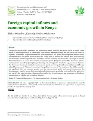
The evolution of migrant remittance inflows to Kenya over the period 1970 to 2014 is shown in Figure 1.
Over this period, remittance inflows increased tremendously from US$7 million in 1970 to US$1.4 billion in
2014. Growth in migrant remittance inflow was minimal in the 1970s. The 1980s witnessed an upward
swing from US$28 million recorded in 1980 to US$79 million in 1982 representing a whopping 183 percent
increase. A peak of US$89 million was recorded in 1989. A further growth in remittance inflows was
recorded over the 1990s rising from US$139 million in 1990 to US$432 million in 1999, representing 210
percent. The average annual increase inflow during this period was US$235 million, an amount much higher
than the total flows in the 1970s and almost 40 percent of the total flows in the 1980s. From 2003 the
country witnessed tremendous growth in remittances from US$538 million recorded in 2000 to US$1.44
billion recorded in 2014. This represented 168 percent increase over the period. While growth in
remittances averaged 27 percent between 2000 and 2010, a remarkable 110 percent increase was recorded
between 2010 and 2014. An average annual increase in inflow of US$151million was recorded during the
later periods of the study. The drop in rate of increase in remittances between 2008 and 2009 could be
attributed to the global financial crisis while the drastic growth could be attributed to the rise in the number
of Kenyans in the Diaspora and improved financial sector developments, among other factors.
1600
1400
Million
1200
1000
800
US$
600
400
200
0
1978
2002
1970
1972
1974
1976
1980
1982
1984
1986
1988
1990
1992
1994
1996
1998
2000
2004
2006
2008
2010
2012
2014
Years
Figure 1. Migrant Remittances Inflows to Kenya 1970-2014
Figure 2 shows the flow of remittances to Kenya for 2014 by source. The inflows are mainly concentrated
in two countries, the United Kingdom and the United States of America, jointly accounting for 64 percent.
During this year, 33 percent of the remittances came from United Kingdom amounting to US$494 million.
Remittance inflows from United States of America were to the tune of US$460 million representing 31
percent of the total inflows. Canada was third with US$98 million representing 7 percent. With the ongoing
efforts at regional integration in East Africa, remittances from two of Kenya's neighbours and members of the
East African Community - Tanzania and Uganda- were among the top five. Remittance inflows from Tanzania
stood at US$96 million representing 6 percent while those from Uganda amounting to US$72 million
represented 5 percent. The foregoing situation implies the sensitivity of the inflows to economic or political
10. International Journal of Development and Sustainability Vol.5 No.8 (2016): 367-
413
shocks in these five countries, particularly the United Kingdom, the United States of America and Canada. At
the East African region, developments in Tanzania and Uganda would impact positively or negatively on the
inflows from these countries.
Others Germany South Africa South Sudan
5% 2% 2% 1% Tanzania
Italy
Uganda 6%
1%
5%
United States Sweden
31% 1%
United
Kingdom
33%
Switzerland
1%
Australia Canada Netherlands
4%
7% 1%
Figure 2. Sources of Remittance Inflows in 2014
2.2. Official development assistance
ODA inflows to Kenya have been much higher than the migrant remittance inflows over the study period as
shown in Figure 3 below.
3500
Million
3000
2500
2000
1500
US$
1000
500
0
1980
1994
2010
1970
1972
1974
1976
1978
1982
1984
1986
1988
1990
1992
1996
1998
2000
2002
2004
2006
2008
2012
2014
Years
Remittances Net official development assistance received
Figure 3. Remittances and ODA (net) 1970-2014
There was a gradual increase in ODA in the 1970s from US$57 million in 1970 to US$348 million in 1979.
The inflows doubled between 1970 and 1974 possibly due to the 1973-1974 oil crisis that necessitated the
increase in demand for foreign exchange to enable the country meet her oil imports. An increase in ODA
12. International Journal of Development and Sustainability Vol.5 No.8 (2016): 367-
413
inflows of US$232 million was recorded between 1974 and 1979. The need to mitigate the effects of the 1975
drought in Kenya partly accounted for the increase in the ODA inflows over this period.
The 1980s marked the period where Kenya together with other developing countries implemented the
Structural Adjustment Programme (SAPs). This period witnessed an increase in ODA flows from US$395
million in 1980 to US$1.06 billion in 1989. This period also marked a frosty relationship between the
Government of Kenya and her international development partners (especially the World Bank and
International Monetary Fund (IMF)) over Kenya’s reluctance to pursue policy reform. This was evidenced by
the Bank’s failure to disburse US$50 million in July 1982 (Njeru, 2003). However, funding resumed in 1984
as a humanitarian response to drought that year, and that this funding was also channelled through the Non-
Governmental Organisation (NGO) sector.
The 1990s marked the clamour for a multi-party democracy and the need for a new constitutional
dispensation. This period also witnessed two stand-offs between Kenya and the donor community – in 1992
and 1997. The ODA inflows during the 1990s declined tremendously from US$1.18 billion in 1990 to US$310
million. It may be noted that much of the flows in the later part of the 1980s from the multilateral agencies
were SAPs related. The drastic decline in ODA inflows in the 1990s could be attributed to the not so good
relationship between President Moi’s government and the donor community. It may be observed from the
graph that migrant remittance inflows was higher than the ODA inflows especially over the period 1999 to
2003 and nearly compared in 2004.
There was commendable growth in ODA flows in the year 2000s. An increase of 28 percent was recorded
between 2000 and 2005. A further increase of 134 percent was recorded between 2005 and 2009. Between
2009 and 2014, ODA inflows increased from US$1.8 billion to US$3.2 billion in 2013. It may be observed that
much of the increase in ODA inflows happened especially after 2002 regime change. Whereas migrant
remittances have been increasing, the rise has been much lower than that of the ODAs especially in the
period after 2000.
2.3. Foreign direct investment
Net FDI inflows to Kenya have generally been low when compared to the previous two types of inflows. The
inflows were also highly volatile and generally declining in the 1980s and 1990s despite the economic
reforms and the progress made in the business environment (Mwega and Ngugi, 2006). Figure 4 shows FDI
net inflows over the period 1970 to 2014.
FDI rose in the 1970s from US$14 million in 1970 to US$84 million in 1979. However, there were
noticeable declines over the period with a low of US$6.3 million being received in 1972. Net FDI inflows
average US$48 million between 1975 and 1979. The early 1980s saw a decline in FDI to US$13million in
1982. It may be recalled that there was an attempted coup in Kenya during August of that year. A further
decline of US$11 million was recorded in 1984 before picking up slightly and declining to the lowest amount
of US$0.4 million in 1988. The 1980s was the period when there was clamour for multi-party democracy in
Kenya while the country was at the same time implementing the Structural Adjustment Programme. The
14. International Journal of Development and Sustainability Vol.5 No.8 (2016): 367-413
political and economic environment obtaining at that time was not conducive for investment. Most investors
therefore shunned the country.
US$ Million
1000.0
800.0
600.0
400.0
200.0
0.0
-200.0
1970
1972
1974
1976
1978
1980
1982
1984
1986
1988
1990
1992
1994
1996
1998
2000
2002
2004
2006
2008
2010
2012
2014
Years
Figure 4. Foreign Direct Investment, net Inflows (1970-2014)
The 1990s saw FDI decline to a low of US$6 million in 1992 before a rise to US$ 146 million in 1993.
Kenya reverted to a multi-party democracy in 1991. The first multi-party elections were held in December
1992. The developments prior to the election made investors to be cagey about possibilities for investing in
the country. This situation accounts for the drastic decline in FDI as investors adopted a wait and see
strategy. The sharp rise in FDI inflows in 1993 confirms the scenario just explained. Another peak of US$108
million was recorded in 1996, a year before the 1997 elections that recorded a decline of US$62 million.
The early part of the 2000s recorded continued fluctuations with a minimum of US$5 Million being
recorded in 2001, a year preceding the 2002 elections. The highest amount of FDI inflows over the period
2000 and 2009 was US$729 million recorded in 2007. The post-election clashes that occurred arising from
the 2007 election led to the decline in FDI inflows in 2008 where US$96 million was recorded. An upward
swing in FDI net inflows has been evident for the period 2010 and 2014. The highest amount of net FDI
inflows to Kenya was recorded in 2014 where a total net inflow of US$944 million was received.
The FDI fluctuations may be due to a number of factors with the first being the recurrent politically
instigated tribal clashes. A case in point is the 1992 and 1997 tribal clashes in the Rift Valley and Coast
Provinces that led Nairobi to be rated as one of the most dangerous cities in the world by the United Nations’
International Civil Service Commission. Second, in the 1990s, Kenya had a frosty relationship with her
development partners that resulted into suspension of any form of financial assistance to the Kenyan
Government by the Bretton Woods Institutions and other bilateral donors who were supporting political
pluralism and good governance. The prevailing situation made Kenya unattractive to investors.
374 ISDS www.isdsnet.com
15. International Journal of Development and Sustainability Vol.5 No.8 (2016): 367-
413
The third factor is the post 2000 emergence of new investments in the mobile telephone sector and the
increased private sector borrowing to finance electricity generation due to drought at the time (Ngugi and
Nyang’oro, 2005). Fourth, the government’s policy shift from import substitution (IS) to export promotion
(EP) led to the establishment of the Export Processing Zone (EPZ) in 1990. The net effect of this policy shift
was increased FDI towards specific industrial sub-sectors such as the garment industry to take advantage of
the African Growth Opportunity Act (AGOA) initiative. The latest increase in FDI is attributed to the interest
by the Chinese in not only the construction industry but also the shift to manufacturing and communications
as witnessed in the setting up of Xinhua News and the China Central Television African headquarters in
Nairobi. The latest upsurge is also attributable to exploration of oil activities in Turkana (IMF, 2012) and the
Titanium mining in Kwale. According to UNCTAD (2014), FDI flows was driven by rising flows to Kenya given
the country’s favoured status as a business hub for oil and gas exploration, industrial production, transport
services and overall infrastructure investments in the sub-region.
2.4. Economic Growth
Kenya has experienced periods of chequered economic growth. High growth performance was registered
from independence in 1963 to the early part of 1980s.The 1980s to 2002, was synonymous with slow or
negative growth, mounting macroeconomic imbalances and a huge increase in poverty and declining life
expectancy. The government’s failure to embrace policy reform coupled with increased role of politics over
policy has been attributed to having contributed to the foregoing situation (Legovini, 2002). There was a
marked economic resurgence between 2003 and 2011 following the 2002 elections and change in the
leadership of the country.
Figure 5 presents trends in Kenya’s economic growth over the study period.
Percent
25.0
20.0
15.0
10.0
5.0
0.0
-5.0
-10.0
1970
1972
1974
1976
1978
1980
1982
1984
1986
1988
1990
1992
1994
1996
1998
2000
2002
2004
2006
2008
2010
2012
2014
Years
Figure 5. Trends in Kenya’s Economic Growth (1970-2014)
The Kenyan economy grew at an average real growth rate of 5 per cent between 1963 and 1970 and at 8
percent between 1970 and 1980. In contrast, the following two decades were characterized by a stagnating
17. International Journal of Development and Sustainability Vol.5 No.8 (2016): 367-
413
economy with average growth rates of 4 and 2 per cent in the periods 1990/80 and 2000/90, respectively.
According to Republic of Kenya (2006), real GDP growth averaged 3.0 percent from 1990 to 2005. In 2006,
Kenya’s GDP was about US$17.39 billion. The country’s real GDP growth picked up to 2.3 percent in early
2004 and to nearly 6 per cent in 2005 and 2006, compared with a paltry 1.4 per cent recorded in 2003 and
throughout President Moi’s last term (1997–2002).
Real GDP was expected to continue to improve, mainly as a result of expansions in key sectors of the
economy such as tourism, telecommunications, transport, construction and anticipated recovery in
agriculture. Real GDP growth rates averaged 4.4 percent over the period 2006 and 2011. The Kenya Central
Bank forecast for 2007 was between 5 and 6 percent GDP growth, but the out turn was 7.1 percent.
Economic growth in the country slumped to 1.7 per cent in 2008 from 7.1 percent in the year 2007. The
subdued growth reflected adverse after-effects of the post-election crisis and high international crude oil
prices, which eventually stifled the transport sector and increased the cost of fuel and energy resources
utilized in several other sectors. Similarly, the global financial crisis that emerged in the last quarter of 2008
further decreased production levels and export demand. In addition, according to the Central Bank of Kenya
(2009), production in the agricultural sector fell due to inadequate rainfall in most parts of the country.
In 2014, Kenya changed the GDP base calculation year to 2009 from 2001. This showed a larger increase
than had been anticipated, pushing the country into the lower ranks of the World Bank’s so-called middle
income nations. This rebasing also meant that the nation’s per capita GDP, the wealth produced annually
divided by the population, increased from US$999 to US$1,246. Kenya’s GDP in 2014 was US$60.9 billion.
3. Methodology
A large body of empirical work on finding relations between macroeconomic fundamentals in terms of
Granger causality forms the first step of this study. The second part examines the short and long-term
relationship of these variables.
Causality suggests a cause and effect relationship between two sets of variables. Granger causality was
introduced by Granger (1969) and has been a popular concept in econometrics. A variable is said to Granger
cause the other if it helps to make a more accurate prediction of the other variable than if the latter's past
was used as a predictor. This causality cannot be interpreted as a real causal relationship but rather shows
how one variable can help to predict the other better. Thus, given two time series variables Xt and Yt, Xt is said
to Granger cause Yt if Yt can be better predicted using the histories of both Xt and Yt than it can by using the
history of Yt alone. We therefore use this approach in modeling the study variables using Pairwise Granger
causality analysis as proposed by Granger (1969).
3.1. Pairwise granger causality tests
We test for the absence of Granger causality by estimating the following Vector Autoregressive (VAR) model:
(1)
19. International Journal of Development and Sustainability Vol.5 No.8 (2016): 367-
413
(2)
Testing against the is a test that Xt does not Granger-cause Yt. On
the other hand, testing against the is a test that Yt does not
Granger-cause Xt.
A rejection of the null hypothesis implies there is Granger causality between the variables. Two variables
are usually analysed together in Granger causality, while testing for their interaction. The four possible
results of the analyses are (i) Unidirectional Granger causality from variable Yt to variable Xt, (ii)
Unidirectional Granger causality from variable Xt to Yt, (iii) Bi-directional causality and (iv) No causality.
3.2. The Model
The overall objective of this study was to examine the impact of foreign capital inflows on economic growth
in Kenya taking into due consideration their volatility and the macroeconomic policy environment. We
follow Fambon (2013) and use an aggregate production function (Yt) that incorporates the foreign capital
inflows and other variables of relevance in the model. The basis for the model is the endogenous growth
model that makes use of the Cobb-Douglas production function as the aggregate production function of the
economy. We therefore assume a Production function of the form:
(3)
where Yt is the output of the economy and represents real per capita GDP at time t; At, Kt and Lt are
respectively the productivity factor, the capital stock, and the labour stock at time t, ε is the disturbance term
and e is a base of natural logs
Our key variables of concern are Remittances, Foreign Aid and Foreign Direct Investment inflows.
Fambon (2013) argues that the impact of Foreign Aid and Foreign Direct Investments on economic growth
may be captured through changes in At thus assuming that At is a function of Aid and FDI. We however argue
that the three variables under consideration (Aid, FDI and Remittances) could impact on economic growth
through the capital stock. We assume that capital is composed of domestic and foreign capital with the
variables under consideration being part of the foreign capital. We assume that the domestic capital (proxied
in some studies by the Gross Domestic Capital Formation (GDFC)) is as given. We consider the two
assumptions in arriving at the following functional relationship:
Yt = f [REMITt , AIDt , FDIt , LABt , POLICYt ], (4)
where Yt is real per capita GDP, REMIT is Migrant remittance as a share of GDP, AID is ODA as a share of GDP,
FDI is Foreign Direct Investment as a share of GDP, LAB is the employed labour force and POLICY is the
macroeconomic Policy variable (see appendix for computation of the policy variable).
Combining equation (3) and (4), we arrive at the following:
(5)
21. International Journal of Development and Sustainability Vol.5 No.8 (2016): 367-
413
where α, σ, δ, β, and θ are constant elasticity coefficients of output relative to Remit, Aid, FDI, LAB and
POLICY and ɛ t is the error term.
Taking logarithms of equation (5) yields:
We re-write Equation (6), in an explicit estimable function as follows:
We in the first case account for volatility of the foreign capital inflows through the inclusion of the
volatility variables in our model. We examine variations in the means as a first check on volatility noting that
the variables presenting the smallest means would be more volatile. We use H-P filter (Hodrick and Prescott,
1997) to extract the trend and cycle components of foreign aid in line with Bulir and Hamann (2001, 2003,
and 2005), Pallage and Robe (2001) and Rand and Tarp (2002). We also adopt the same approach for the FDI
and the Remittances variables. The H-P filter decomposes a series, xt (where xt is the logarithm of the
observed series Xt) in a cycle, xtc and a trend xtg by minimizing the following equation:
(8)
where is the smoothing parameter of xt
g
and its selection is dependent on the frequency of observations.
Different studies (Bulir and Hamann, 2001; Pallage and Robe, 2001; Ravn and Uhlig, 2002) have
experimented with different values for varying from 7, 100 and 6.25 respectively. In order to arrive at the
best results, this study experimented with each of these values of and opted to use equals 100 in line with
Pallage and Robe (2001) as it represented a better fit.
Our choice of the HP filter is further driven by the conclusion from previous studies that some of the
variables could either be contra-cyclical or pro-cyclical and could either be correlated with the cycles of
national income or fiscal revenues or not (see Bulir and Hamann 2001, 2003, 2005; Pallage and Robe, 2001).
We therefore rewrite Equation (7) above to account for volatility.
(9)
where AHP100 is a measure of Aid volatility, FHP100 is a measure of FDI volatility, RHP100 is a measure of
remittances volatility and all other variables are as previously defined.
We develop an additional model by using another measure of foreign capital inflow volatility derived
from the conditional standard errors of the General Autoregressive Conditional Heteroskedasticity (GARCH)
(see Serven, 2002; Lensink and Morrissey, 2006; Ngugi, 2013 and the graphical representation in Appendix
Figures A2, A3 and A4).
We modify equation (9) to include three new measures of volatility:
23. International Journal of Development and Sustainability Vol.5 No.8 (2016): 367-
413
(10)
where AIDVOL is a measure of Aid volatility, FDIVOL is a measure of FDI volatility and REMITVOL is a
measure of volatility of remittances.
As a robustness test for our results, we interacted key variables in (6) with the policy variable to
understand their effects on growth given the prevailing macroeconomic policy environment in line with
previous aid studies (Burnside and Dollar, 1997; World Bank, 1998; Ojiambo et al., 2015). We modify
Equation 6 as follows:
(11)
where AIP is an interaction of the Aid and the macroeconomic policy variable, FIP is an interaction of the FDI
and the macroeconomic policy variable, RIP is an interaction of the Remittances and the macroeconomic
policy variable and all other variables are as previously defined.
3.3. The estimation technique
Engle and Granger (1987) two-step method has been commonly used in parameter estimation in a
cointegration system. The autoregressive distributed lag (ARDL) model as developed by Pesaran and Shin
(1995, 1999), Pesaran et al. (1996), and Pesaran (1997) combined the Engle and Granger two step-procedure
into one step in a bid to examine the direction of causation between the variables. This approach has
advantages over the Johansen (1988) and Johansen and Juselius (1990). Whereas the conventional
cointegration approach estimates the long-run relationships within the context of a system of equations, the
ARDL approach employs a single reduced form equation (Pesaran and Shin, 1995). The approach also yields
precise estimates of long-run parameters and valid t-statistics even in the presence of endogenous variables
(Inder, 1993). Additionally, the ARDL approach does not necessarily require pre-testing of the variables,
implying that the test is possible even if the underlying regression is purely I(0), purely I(1) or a mixture of
the two. This uniqueness of the approach makes it superior to the other methods as the time series data are
in most cases integrated of the same order. The ARDL approach also avoids the large number of
specifications necessary for conventional cointegration tests. Some of these include the number of
endogenous and exogenous variables (if any) to be included in the model, the differences in order of
integration of variables, and the treatment of deterministic elements and the number of lags.
According to Pesaran and Smith (1998), the results of the conventional cointegration tests are generally
very sensitive to the method and various alternative choices available in the estimation procedure. However,
under the ARDL approach, it is possible to have different optimal lags that could be used with limited sample
data (30 variables), making it quite suitable for this study. According to Ghatak and Siddiki (2001), the ARDL
model is, therefore, more statistically significant approach to determine the cointegration relation in small
25. International Journal of Development and Sustainability Vol.5 No.8 (2016): 367-413
samples. From equation (9), the conditional ARDL (r, s1, s2, s3, s4, s5, s6 s7, s8 ….) long-run model for our basic
model was estimated as:
α α α α α α α
α α α
where r, s1, s2, s3, s4, s5, s6 s7, s8 are the lag lengths for each of the variables and variables in small letters are
logarithmic transformations.
The conditional ARDL (u, v1, v2, v3, v4, v5…..) long-run model for the second model (from equation 10) was
estimated as:
β β β β β β β
β β β
where u, v1, v2, v3, v4, v5, v6,v7, v8 are the lag lengths for each of the variables.
From equation (9) the conditional ARDL (p, q1, q2, q3, q4, q5, q6, q7, q8) long-run model for the third model
(robustness check model) was estimated as:
δ δ δ δ δ δ δ
δ δ δ
where p, q1, q2, q3, q4, q5, q6, q7, q8 are the lag lengths for each of the variables.
The short-run dynamic parameters were obtained by estimating an error correction model associated
with the long-run estimates. This was specified as follows for the three models:
θ θ θ θ θ θ
θ θ θ θ
φ φ φ φ φ φ
380 ISDS www.isdsnet.com
26. International Journal of Development and Sustainability Vol.5 No.8 (2016): 367-
413
φ φ φ φ
where θ (1…9), φ (1…..9) and φ (1….9) are the short-run dynamic coefficients of the model’s convergence to
equilibrium, and πs are the speed of adjustment to long-run equilibrium following a shock to the system.
The orders of the lags in the ARDL model are selected using either Akaike information criteria (AIC) or the
Schwartz-Bayesian information criteria (SIC or SBC). According to Shrestha and Chowdhury (2005), the
model selection criterion is a function of the residual sums of squares and is equivalent asymptotically. This
study used the SBC to select the orders of the ARDL specifications due to its comparative advantages over the
AIC (Kargbo, 2012). Pesaran and Shin (1999)'s comparison of AIC and SIC in the Monte Carlo experiments
they ran showed that though the ARDL-AIC and ARDL-SBC had quite similar small-sample properties, the
ARDL-SBC performed slightly better in the majority of the experiments. Therefore, they suggested that this
could be due to the fact that the Schwartz criterion was a consistent model selection criterion whereas the
Akaike was not. Thus, the SBC is more parsimonious with the lag length selection and is a consistent model
selection criterion. This also ensured that degrees of freedom were not lost given the number of observations
in the study.
4. Data sources and characteristics
4.1. Data source and definition
The study used secondary sources of data covering the period 1970 – 2014. The data on Foreign aid, real
GDP, migrant remittances Inflation, Final Government consumption and degree of openness were obtained
from the World Bank, Africa Development Indicators database. Foreign Direct Investment (FDI) data was
obtained from UNCTAD. Variable definition and measurement are shown in Appendix Table A1.
4.2. Descriptive statistics and correlation results
The raw data makes it hard to visualise what the data is showing hence, descriptive statistics are important
in presenting the data in a more meaningful way that allows for simpler interpretation. The results of the
descriptive statistics of the variables used in the study are presented in Appendix Table A2. Examination of
28. International Journal of Development and Sustainability Vol.5 No.8 (2016): 367-
413
the mean and standard deviations, show that there was no case where the standard deviation was greater
than the mean. This therefore implied that the mean was a good estimator of the parameters. All the major
variables under consideration are skewed to the right an evidence of a distribution where the mean is
greater than the median. Kurtosis is greater than 3 for all variables under consideration (except remittances
and labour), indicating that the distribution of each series is flatter than the Gaussian distribution. It is clear
that the Jarque-Bera test rejects the null hypothesis of a Gaussian distribution due to its high values. The
correlation matrix for the variables is presented in Appendix Table A3. The correlation coefficient lies
between +1 and -1. The correlation coefficient is positive when the two variables tend to move in the same
direction and negative when the two variables tend to move in the opposite directions.
4.3. Unit root tests and cointegration
Prior to conducting the tests, we examined the statistical properties of the data and cointegration. In most of
similar works, and to examine the possible causality relations between the variables of interest and the short
and long run relationships, the statistical properties of the data must be first checked for stationarity and
cointegration. We diagnosed the stationarity by conducting a unit root test (using Augmented Dickey Fuller
and Phillips-Perron). Cointegration was performed using Johansen (1988) procedures and the bound testing
procedure as developed by Pesaran and Pesaran (1997). These tests therefore formed a critical basis for our
empirical work.
4.3.1. Unit root test
The data used in this study was recorded over the period 1970 and 2014. A basic assumption when
conducting regression on time series data is that the data series must be stationary. Thus, a test for the
existence of unit roots for each series using the Augmented Dickey-Fuller (ADF) and Phillips-Perron was
done.
Time series data generally tend to be non-stationary in nature or have unit roots. A non-stationary series
may have a number of unit roots and is often referred to as integrated to the order of d [I (d) where d = 1,
2…]. A stationary series is said to be integrated to the order of 0 [I(0)]. There are important differences
between non-stationary and stationary time series in terms of their responses to shocks. Shocks to a
stationary time series are temporary, over time the effects of the shocks will dissipate and the series will
revert to its long term equilibrium level. As such, forecasts of a stationary series will converge to the mean of
the series. Shocks to a non-stationary series persist over time, since the mean and variance of a non-
stationary series are time dependent. As a result of non-stationarity, regressions with time series data are
likely to result in spurious results.
In light of the above, the study tested for the existence of unit roots for each series using the Augmented
Dickey-Fuller (ADF) and Phillips-Perron. The ADF is an extension of the simple Dickey-Fuller (DF) method.
The results of these tests are shown in Table 1 and 2 below.
30. International Journal of Development and Sustainability Vol.5 No.8 (2016): 367-
413
Table 1. ADF Unit root test results
Level First difference
Variables Constant and Constant Constant and Constant and Conclusions
no trend and trend no trend trend
logY -0.7885 -1.9879 -3.4256** -3.4061** I(1)
logREMIT -1.2134 -1.8672 -5.9385* -5.8785* 1(1)
logAID -1.6841 -1.7265 -3.8982** -3.8798** I(1)
logFDI -5.2497* -5.2965* - - I(0)
LogPOLICY -3.0809** -3.4600** - - I(0)
logLAB 0.1363 -1.5095 -4.0477** -3.9975** I(1)
AHP100 -3.5213** -3.4477** - - I(0)
FHP100 -5.3736* -5.2533* - - I(0)
RHP100 -3.6444* -3.54045** - - I(0)
Note: * and ** indicate statistical significance at the 1% and, 5% levels of significance, respectively
According to the ADF test as shown in Table 1, variables were integrated of order 1 or 0. Four of the
variables (LY, LREMIT, LAID and LLAB) were integrated of order 1 while the rest were integrated of order 0
(I (0)). The dependent variable (logarithm of real per capita income) was integrated of order one (I (1)),
therefore, implying that an ARDL could be used to estimate the model (Pesaran and Shin, 1995; 1999). ARDL
model can be estimated so long as the dependent variable is I(1) and independent variables can either be
I(1) or I(0) or a mix.
We further examined the validity of the above conclusions using the Phillips-Perron Unit Root test. Its test
statistics can be viewed as Dickey–Fuller statistics that have been made robust to serial correlation by using
the Newey and West (1987) heteroscedasticity and autocorrelation-consistent covariance matrix estimator.
The advantages of the PP tests over the ADF tests is that the PP tests are robust to general forms of
heteroscedasticity in the error term ut and the user does not have to specify a lag length for the test
regression. The results of PP are presented in Table 2.
The table shows that the PP results are a confirmation of those found using the ADF. We can therefore
conclude that the variables are integrated of a mixed order and that none of them is integrated of order 2 (I
(2)). We therefore satisfy the requirement that unit root tests in the ARDL procedure may still be needed to
make sure that none of the variables is integrated of order 2 or beyond. With this having been confirmed, we
can confidently apply the ARDL bounds tests to our model.
32. International Journal of Development and Sustainability Vol.5 No.8 (2016): 367-
413
Table 2. Phillips-Perron (PP) Unit root test results
Level First difference
Variables Constant and Constant and Constant and Constant Conclusions
no trend trend no trend and trend
logY -0.6825 -1.7251 -4.4952* -4.4434* I(1)
logREMIT -1.4052 -2.1461 -7.8271* -7.8116* 1(1)
logAID -1.9078 -1.9211 -6.6460* -6.5891* I(1)
logFDI -7.0423* -7.0280* - - I(0)
logPOLICY -3.3938** -3.6913** - - I(0)
logLAB 0.0833 -1.6718 -6.6231* -6.5666* I(1)
AHP100 -4.2822* -4.2228* - - I(0)
FHP100 -5.7108* -5.5199* - - I(0)
RHP100 -3.4541** -3.3756** - - I(0)
Note: * and ** indicate statistical significance at the 1% and, 5% levels of significance, respectively
4.3.2. Cointegration analysis
The essence of a cointegrating relationship is that the variables in the system share a common unit root
process. This methodology is also particularly suitable in this context because it provides a flexible functional
form for modelling the behaviour of the variables under the long-run equilibrium condition. This approach is
also appealing because it treats all variables as endogenous; it thus avoids the arbitrary choice of the
dependent variable in the cointegrating equations. We adopt two approaches to cointegration, Johansen
(1988) procedures and the bound testing procedure as developed by Pesaran and Pesaran (1997).
In Johansen's procedure, we assume no deterministic trend and we first test the hypothesis that there are
no cointegrating relations (number of cointegrating vectors, r = 0) and then the hypothesis of at most one
cointegrating vectors all the way to eight. These hypotheses are tested by comparing the trace statistic with
the 1% and the 5% critical values. Table 3 confirms the existence of cointegration between these variables of
interest in our study.
The study also used the bound testing procedure as developed by Pesaran and Pesaran (1997). This is the
first step in an ARDL approach as it makes it possible to determine whether there exists a long-run relation
between the variables. In this regard, the hypothesis of no cointegration was tested. The null hypothesis in
this case is that the coefficients on the lagged regressors (in levels) in the error-correction form of the
underlying ARDL model are jointly zero. The null hypothesis is defined by H0: δ1 = δ2 = 0 and tested against
the alternative of H1: δ1 ≠ 0; δ2 ≠ 0 (where δ1, δ2 are the coefficients of the lagged regressors). Critical values
are provided by Pesaran and Pesaran (1997). The calculated F-Statistic of logY, logAID, logFDI, logREMIT,
34. International Journal of Development and Sustainability Vol.5 No.8 (2016): 367-
413
logPOLICY and logLAB is given as 2.8924 (0.037). The F-Statistic falls between the 95 percent critical values
(of Case II: intercept and no trend) as provided by Pesaran and Pesaran (1997) that is, 2.476 if the variables
are I (0) and 3.646 if variables are I (1). Its significance is evidenced by a p-value of 0.037. We accept the
results given that the variables were found to be integrated in a mixed order.
Table 3. Johansen Cointegration Test Results
Test assumption: No deterministic trend in the data
Series: logYlogAIDlogFDIlogREMITlogPOLICYlogLAB AHP100 FHP100 RHP100
Likelihood 5 Percent 1 Percent Hypothesized
Eigen value Ratio Critical Value Critical Value No. of CE(s)
0.7858 261.5944 175.77 181.44 None **
0.7148 195.3348 141.2 152.32 At most 1 **
0.6078 141.3813 109.99 119.8 At most 2 **
0.4951 101.1298 82.49 90.45 At most 3 **
0.4600 71.7479 59.46 66.52 At most 4 **
0.3439 45.25223 39.89 45.58 At most 5 *
0.3393 27.1314 24.31 29.75 At most 6 *
0.1813 9.3109 12.53 16.31 At most 7
0.0164 0.7107 3.84 6.51 At most 8
*(**) denotes rejection of the hypothesis at 5%(1%) significance level
L.R. test indicates 7 cointegrating equation(s) at 5% significance level
5. Empirical results
5.1. Granger causality
Table 4 presents the results of the pairwise Granger causality test which stand as empirical facts. The table
shows that there is uni-directional causality between GDP per capita and FDI, Labour and GDP per capita and
Labour and Foreign Aid. These results give credence to the earlier results on Johansen Cointegration
technique that found the existence of 7 cointegration equations in the variables in the study. It may be
inferred from these findings that economic growth is good for growth in FDI and the country’s labour force.
38. International Journal of Development and Sustainability Vol.5 No.8 (2016): 367-
413
Pairwise Null Hypothesis: Obs F-Statistic Prob. Decision Type of Causality
( implies does not Granger cause)
logPOLICYlogAID 43 2.3864 0.1056 DNR H0 No causality
logAIDlogPOLICY 43 0.9167 0.4085 DNR H0 No causality
logLABlogFDI 43 0.3214 0.7271 DNR H0 No causality
logFDIlogLAB 43 0.9813 0.3841 DNR H0 No causality
logPOLICYlogFDI 43 2.9024 0.0671 DNR H0 No causality
logFDIlogPOLICY 43 1.5663 0.2220 DNR H0 No causality
logPOLICYlogLAB 43 0.1797 0.8362 DNR H0 No causality
logLABlogPOLICY 43 1.7778 0.1828 DNR H0 No causality
Alpha (α) = 0.05 Decision rule: reject H0 if P-value < 0.05. Key: DNR = Do not reject
5.2. Results of ARDL estimation
We separately estimate Equations (9) through (11) and use SBC in selecting the lag length on each of the first
differenced variable. The estimates of the ARDL representation are summarized in Appendix Table A5 as
Model A, B and C.
5.2.1. Diagnostic tests
Diagnostic testing has become an integral part of model specification in econometrics. There have been
several important advances over the past 20 years. Various diagnostic tests were conducted to ensure that
the coefficients of the estimates were consistent and could be relied upon in making economic inferences.
Diagnostic tests for autoregressive conditional heteroscedasticity, serial correlation, functional form and
heteroscedasticity were conducted. In this respect, the study used Breuch-Godfrey lagrange multiplier (LM)
for serial correlation, the lagrange multiplier test for conditional heteroscedasticity (ARCH) were used on the
residuals to determine the OLS assumption on the error term. The Ramsey RESET test was conducted for the
correct specification of the error-term. The Jarque-Berra statistic was used to determine whether the sample
data have the skewness and kurtosis matching a normal distribution. Table 5 shows the results of the
diagnostic tests.
The table shows that there was no evidence of autocorrelation in the disturbance of the error term and
the ARCH tests suggest the errors were homoskedastic and independent of the regressors. All models passed
the Jarque-Bera normality tests suggesting that the errors are normally distributed. The RESET test indicated
that the models were correctly specified.
40. International Journal of Development and Sustainability Vol.5 No.8 (2016): 367-413
Table5. Results of Diagnostic Tests
Model A
Diagnostic Tests
Test Statistics LM Version F Version
A: Serial Correlation CHSQ (1) = 0.7283(0.393) F (1, 24) = 0.4135(0.526)
B: Functional Form CHSQ (1) = 0.3938(0.530) F (1, 24) = 0.2218(0.642)
C: Normality CHSQ (2) = 1.0217(0.600) Not applicable
D: Heteroscedasticity CHSQ (1) = 1.9449(0.163) F (1, 41) = 1.9423(0.171)
Model B
Test Statistics LM Version F Version
A: Serial Correlation CHSQ (1) = 0.1953(0.659) F (1, 23) = 0.1101(0.743)
B: Functional Form CHSQ (1) = 1.2647(0.261) F (1, 23) = 0.7320(0.401)
C: Normality CHSQ (2) = 1.6815(0.431) Not applicable
D: Heteroscedasticity CHSQ (1) = 0.2366(0.627) F (1, 39) =0.2264(0.637)
Model C
Diagnostic Tests
Test Statistics LM Version F Version
A: Serial Correlation CHSQ (1) = 0.2134(0.644) F (1, 28) = 0.1396(0.711)
B: Functional Form CHSQ (1) = 3.1943(0.074) F (1, 28) =2.2469(0.145)
C: Normality CHSQ (2) = 0.3304(0.848) Not applicable
D: Heteroscedasticity CHSQ (1) = 0.7040(0.401) F (1, 41) =0.6825(0.414)
5.2.2. Stability tests
The study examined the stability of the long-run parameters together with the short-run movements for the
equation and relied on cumulative sum (CUSUM) and cumulative sum of squares (CUSUMSQ) tests as
388 ISDS www.isdsnet.com
41. International Journal of Development and Sustainability Vol.5 No.8 (2016): 367-413
proposed by Borensztein et al. (1998). This same procedure has been utilized by Pesaran and Pesaran
(1997), Suleiman (2005), and Bahmani-Oskooee and Ng (2002) to test for the stability of the long-run
coefficients. According to Pesaran and Pesaran (2009), the CUSUM test is particularly important for detecting
systematic changes in the regression coefficients, while the CUSUMSQ test is useful in situations where the
departure from the constancy of the regression coefficients is haphazard and sudden.
Plot of Cumulative Sum of Recursive Residuals
20
10
0
-10
-20
1972 1983 1994 2005 2014
The straight lines represent critical bounds at 5% significance level
Plot of Cumulative Sum of Squares of Recursive Residuals
1.4
1.2
1.0
0.8
0.6
0.4
0.2
0.0
-0.2
-0.4 Figure 6. Plot of CUSUM and
1972 1983 1994 2005 2014 CUSUMSQ for Model AUnlike the Chow test that requires break point(s) to be specified, the
The straight lines represent critical bounds at 5% significance level
CUSUM tests can be used even if the structural break point is not known. Thus, the CUSUM test uses the
cumulative sum of recursive residuals based on the first n observations and is updated recursively and
plotted against break point. The CUSUMSQ makes use of the squared recursive residuals and follows the
same procedure. When the plot of the CUSUM and CUSUMSQ stays within the 5 per cent critical bound, the
null hypothesis that all coefficients are stable cannot be rejected. However, when either of the critical
ISDS www.isdsnet.com 389
42. International Journal of Development and Sustainability Vol.5 No.8 (2016): 367-
413
boundary lines are crossed, then the null hypothesis (of parameter stability) is rejected at the 5 per cent
significance level. Figure 6, 7 and 8 presents the plots of CUSUM and CUSUMSQ for the two models.
Plot of Cumulative Sum of Recursive Residuals
20
10
0
-10
-20
1974 1984 1994 2004 2014
The straight lines represent critical bounds at 5% significance level
Plot of Cumulative Sum of Squares of Recursive R esiduals
1.4
1.2
1.0
0.8
0.6
0.4
0.2
0.0
-0.2
-0.4
Figure 7. Plot of CUSUM and
1974 1984 1994 2004 2014
The straight lines represent critical bounds at 5% significance level
CUSUMSQ for Model B
It can be seen from the figures that the plot of CUSUM stays within the critical 5 per cent bound and
CUSUMSQ statistics does not exceed the critical boundaries that confirms the long-run relationships between
the economic growth and the variables. It also shows that the stability of co-efficient plots lie within the 5 per
cent critical bound, thus providing evidence that the parameters of the model do not suffer from any
structural instability over the study period. From the foregoing diagnostic tests, it is clear that the model
passed all the required tests and thus paving way for interpretation of estimates of both the short-run and
long-run coefficients as required in an ARDL approach. It is therefore on the basis of these tests that it was
reasonable to conclude that the model had a good statistical fit.
44. International Journal of Development and Sustainability Vol.5 No.8 (2016): 367-
413
Plot of Cumulative Sum of Recursive Residuals
20
10
0
-10
-20
1972 1983 1994 2005 2014
The straight lines represent critical bounds at 5% significance level
Plot of Cumulative Sum of Squares of Recursive Residuals
1.4
1.2
1.0
0.8
0.6
0.4
0.2
0.0
-0.2
-0.4
1972 1983 1994 2005 2014
The straight lines represent critical bounds at 5% significance level
Figure 8. Plot of CUSUM and
CUSUMSQ for Model C
5.2.3. The short-run results
The empirical results of the short run error-correction model (ECM) results are presented in Table 5. The
table shows that the calculated F-Statistic for the models is a above the critical levels giving credence to the
existence of the long run relationship. The coefficient of the adjustment term (ecm (-1)) is significant at 1 per
cent level and carries the expected negative sign. For the first model, the coefficient is found to be -0.390,
suggesting that that the deviation from the long-term in economic growth is corrected by 39 per cent in the
coming year. This means that an exogenous shock to the economy dissipates completely within two and half
years. The coefficient for the adjustment term is -0.462 implying that deviation from the long-term path is
corrected by 46 percent in the coming year. This is a moderate speed of adjustment, much better than in the
first model. The speed of adjustment for the third model is -0.304. This gives us a much lower rate such that
46. International Journal of Development and Sustainability Vol.5 No.8 (2016): 367-
413
deviation from the long-term economic growth is corrected by 30 percent the following year. Overall, it may
be deduced that the relatively slow speed of adjustment could be attributed to the structural rigidities - lack
of access to productive land, lack of capital, problem of enclave formal economies, export of raw materials,
policy distortions - that are inherent in developing countries such as Kenya, which slows down the
adjustment process as intimated by M’Amanja and Morrissey (2005) and Ojiambo et al.(2015).
Table 5. Error Correction Representation for the Selected ARDL Model
Dependent variable is dy
Accounting for policy
Accounting for volatility Environment
Model A Model B Model C
Regressor Coefficient Coefficient Coefficient
dy1 0.2979*** - -
(0.1067)
dremit -0.1538*** -0.1024*** -0.1114
(0.0396) (0.0348) (0.1214)
dremit1 0.1195*** -0.2095** 0.0711*
(0.0435) (0.0822) (0.0364)
daid -0.1842** -0.1249** 0.3715***
(0.0864) (0.0618) (0.0995)
dfdi -0.0232* -0.020261** 0.0048
(0.0125) (0.0097) (0.0559)
dfdi1 0.0272** 0.0333*** -
(0.0116) (0.0107)
dpolicy -0.1046 -0.1781* 0.7703***
(0.0973) (0.1005) (0.2146)
-0.3554* -0.3338 0.2842***
dlab (0.1972)
(0.1849) (0.0511)
50. International Journal of Development and Sustainability Vol.5 No.8 (2016): 367-
413
Dependent variable is dy
Accounting for policy
Accounting for volatility Environment
Model A Model B Model C
Regressor Coefficient Coefficient Coefficient
2.5692 3.9741 2.1747 3.4537
dy1 = y(-1)-y(-2) dremit1 = remit(-1)-remit(-2) dfdi1 = fdi(-1)-fdi(-2)
Note: Subscript (-1) after a variable identifies the lag; ***, ** and * indicate statistical significance at the 1%,
5% and 10% levels of significance, respectively. d is the first difference operator
It is evident from the table that remittances have a negative effect on economic growth in the short run
implying that a 1 percent increase in remittances would lead to a 0.15 percent decline in economic growth.
This finding is confirmed also in the second model with a slightly reduced but statistically significant negative
coefficient. It is further confirmed in the third model although the coefficient is not statistically significant.
The negative coefficient of remittances in the short-run may be due to the role of remittances in meeting
domestic requirements and their use as an instrument against short-run cyclical fluctuations. This finding is
in line with Qayyum et al. (2010), Al Khathlan (2012), Hassan et al. (2012), Waqas (2013) and Oshota (2014).
A unique finding is in the coefficient of the lagged remittance variable that is positive and statistically
significant at 1 percent level of significance in the first model and at 10 percent in the third model. It implies
that a 1 percent increase in remittances have the potential to increase economic growth by 0.1 percent the
following year. This is a strong evidence of a non-linear relationship. This could be due to unproductive use of
remittances in the beginning followed by more productive utilization as found by Hassan et al. (2012). The
second model finds the coefficient of remittances to be negative and statistically significant even after one
year, a further confirmation of the findings from other studies on this negative relationship.
The coefficient of the Foreign aid is found to be negative and statistically significant at 5 percent level of
significant in the short run in the the first two models but positive and statistically significant at 1 percent
when the macroeconomic policy environment is fully accounted for. Whereas a percentage increase in
foreign aid would result in a 0.2 percent decline in economic growth only when volatility is accounted for,
this situation is improved to 0.4 percent when the macroeconomic policy environment is accounted for. This
finding resonates well with the debate that has existed on conditionality of aid-growth nexus on
macroeconomic policy (Burnside and Dollar, 1997; World Bank, 1998; Oshota, 2014; Ojiambo et al., 2015;
among others). The study also found that the coefficient of the macroeconomic policy variable was positive
and statistically significant in the third model, negative but insignificant in the first model and negative and
statistically significant in the second model. The foregoing implies that a sound macroeconomic policy
environment is good for economic growth.
52. International Journal of Development and Sustainability Vol.5 No.8 (2016): 367-
413
The coefficient of Foreign Direct Investment is negative and statistically significant at 10 percent level of
significance in the first model and at 5 percent level of significance in the second model (when volatility is
accounted for) and positive and insignificant when the macroeconomic policy environment is accounted for.
It is observed that FDI affects economic growth positively but with a lag. From the first model, the coefficient
of the lagged FDI variable is positive and statistically significant at 5 percent level of significance implying
that a percentage increase in FDI would lead to a 0.03 percent increase in economic growth the following
year. This effect is confirmed also in the second model, where this coefficient is positive and statistically
significant at 1 percent level of significance. This is in line with economic theory as investments take time. It
confirms the findings of Lensink and Morrissey (2006) that FDI has a positive effect on growth, though it is
weaker for developing countries. It also corroborates Ngeny and Mutuku (2014) finding on FDI-growth
nexus in Kenya. We also found that the employed labour force variable had a short run negative effect on
economic growth in the first model and a positive and statistically significant coefficient in the third model.
5.2.4. Long-run estimation
Table 6 presents the estimated long run coefficients of the models.
Table 6. Estimated Long Run Coefficients
Dependent variable is y
Accounting for Volatility Accounting for Policy Environment
Model A Model B Model C
Regressor Coefficient Coefficient Coefficient
remit -0.8096*** -0.7068*** -1.5142***
(0.1188) (0.0818) (0.5889)
Aid 0.1841** 0.1454** 1.6313***
(0.0875) (0.0650) (0.3879)
Fdi -0.1396* -0.1429** 0.0016
(0.0802) (0.0602) (0.1836)
policy -0.2704 -0.3859* 2.5304***
(0.2383) (0.1978) (0.9024)
Lab 0.9782*** 0.9107*** 0.9335***
(0.0803) (0.0560) (0.0718)
RHP100 0.0009* - -
54. International Journal of Development and Sustainability Vol.5 No.8 (2016): 367-
413
Dependent variable is y
Accounting for Volatility Accounting for Policy Environment
Model A Model B Model C
(0.0005)
FHP100 0.0002 - -
(0.0002)
AHP100 -0.0003 - -
(0.0003)
REMITVOL - 7.0550*** -
(1.6770)
AIDVOL - -1.1707 -
(13.856)
FDIVOL - -0.9592* -
(0.5257)
AIP - - -0.0368***
(0.0097)
FIP - - 0.0011
(0.0043)
RIP - - 0.01945
(0.0130)
INPT -0.8168 -0.12816 -10.5760***
(1.2508) (3.1960) (3.4508 )
Note: ***, ** and * indicate statistical significance at the 1%, 5% and 10% levels of significance, respectively.
Standard Error in parenthesis
The table shows that the coefficient of the remittances variable was negative and statistically significant at
1 percent level of significance in all the three models. The coefficient of the remittances when volatility is
taken into consideration are marginally different. For example, a 1 percent increase in remittances could lead
to 0.8 percent decline in economic growth in the first model and 0.7 percent according to the second model.
56. International Journal of Development and Sustainability Vol.5 No.8 (2016): 367-
413
This finding is a further confirmation of the short-run results. These findings support those of Chami et al.
(2005), Barajas et al. (2009) and Siddique et al. (2010) in the case of India and Bangladesh and contradict
those of Ocharo (2015), Fayissa and Nsiah (2010) and Siddique et al. (2010). Thus the assertion by Rahman
et al. (2006) that remittances may be used for conspicuous consumption rather than for the accumulation of
productive assets can probably not be ruled out. The long run effect therefore could depend on the
investments made from the remittances received and the relationship between such investments and
economic growth. It may be observed that when volatility is not taken into consideration in the model, the
long run effect of remittances on economic growth is much larger than when it is factored. This point to the
need to ensure that remittance volatility should be factored in models for there to be an accurate measure of
its growth effects.
Results show that the elasticity of foreign aid was positive and statistically significant at 5 per cent in the
long-run in the first two models and 1 percent in the third model. The implication of this is that a 1 percent
increase in foreign aid would result in a 0.18 percent and 0.14 percent increase in economic growth in the
long-run when the macroeconomic policy environment is not fully accounted for as in the first two models
and 1.6 percent in the third model. The study finding is in line with other studies such as Mosley (1980),
Singh (1985), Mosley et al. (1987), Snyder (1993), Murthy et al. (1994), Gounder (2001), Lloyd et al. (2001),
Mavrotas (2002), M’Amanja and Morrissey (2005), Karras (2006), Bhattarai (2009), Kargbo (2012) and
Ojiambo et al. (2015).
The coefficient of Foreign Direct Investment is negative and statistically significant at 10 percent level of
significance in the first model, at 5 percent in the second and positive but statistically insignificant in the
second model. The negative relationship between FDI and economic growth is in line with the findings by
Haddad and Harrison (1993), Aitken and Harrison (1999), Levine and Carkovic (2002), and Fortanier (2007).
This could be explained by the limited FDI inflows to Kenya over the study period and the fact that the
prevailing political and macroeconomic environment has not been conducive to FDI inflows. As explained
earlier, there has over the period been noticeable decline in FDI inflows into Kenya during election years as
investors have been cagey about the future of their investments.
6. Conclusion
Kenya has over the period been receiving Foreign Aid, FDI and Remittances. These capital inflows bring in
large amounts of foreign currency that help sustain the balance of payments. While a dearth of studies have
sought to examine the effect of each of these forms of foreign capital inflows on economic growth, the results
have been mixed. Not many have examined the effect of the capital inflows on economic growth within the
same model while taking into cognisance their volatility and the macroeconomic policy environment. While
appreciating the nature of debate that has existed on the nexus between each of the various forms of foreign
capital inflows with economic growth, we however did not seek to settle the debate. We used both granger
causality and ARDL to examine the relationship.
58. International Journal of Development and Sustainability Vol.5 No.8 (2016): 367-
413
We observe that foreign capital is supposed to accelerate economic development of developing countries
to a point where a satisfactory growth rate can be achieved on a self-sustaining basis. This being the case
then private capital inflows in the form of private investment; foreign investment, foreign aid and private
bank lending are the principal ways by which these resources flow from developed/developing to
developing/developed economies albeit at varying levels.
We found that there is uni-directional causality from GDP per capita to FDI, employed labour to GDP per
capita and employed labour to foreign aid. This could be interpreted to imply that economic growth is good
for growth in FDI and the country’s labour force is important in the growth of the country’s GDP. Such a
growth could spur FDI inflows thereby leading to employment creation. It can also be said that the country’s
labour force is important in the best utilization of foreign aid.
We note that the short-run effect of remittances on economic growth is initially negative owing to
possibilities of these inflows being used to finance consumption. However, the full magnitude of this effect is
evident after one year. This non-linear relationship could be attributed to unproductive use of remittances in
the beginning followed by more productive utilization as found by Hassan et al. (2012). The long-run effects
of remittances are negative. Thus the assertion by Rahman et al. (2006) that remittances may be used for
conspicuous consumption rather than for the accumulation of productive assets can probably not be ruled
out. The long run effect therefore could depend on the investments made from the remittances received and
the relationship between such investments and economic growth.There is therefore need to ensure that
remittances are directed towards productive investments in the country. The Government of Kenya should
thus provide viable investment opportunities for citizens from the diaspora in order for such inflows to have
a significant impact.
The short-run effect of foreign aid on economic growth is negative when the macroeconomic policy
environment is not fully accounted for but positive when it is. This implies that a sound macroeconomic
policy environment is important for foreign aid effectiveness.
FDI inflows to Kenya have been volatile over the study period. While FDI inflows is supposed to have a
positive effect on economic growth, we find a negative effect when volatility is accounted for but positive
(but insignificant) when the macroeconomic policy environment is fully accounted for. This finding is a
confirmation of what other studies have found that foreign direct investment has a positive effect on growth,
though weaker for developing countries. This calls for the Government of Kenya to provide incentives that
will attract more FDI inflows contangent on sound macroeconomic policy environment. The need to shift
away from aid to FDI could be a better way of enhancing the possible positive effects of FDI on economic
growth. The current government efforts of marketing Kenya as an investment destination could help in
increasing the inflows.
References
Acemoglu, D., Johnson, S. and Robinson, A. (2001), “The colonial origins of comparative development: An
empirical investigation”, American Economic Review,Vol. 91, pp. 1369-1401.
60. International Journal of Development and Sustainability Vol.5 No.8 (2016): 367-
413
Adeniyi, O., Omisakin,O., Egwaikhide, F.O. and Oyinlola, A.(2012), “Foreign Direct Investment, economic
Growth and Financial Sector Development in Small Open Developing Economies”, Economic Analysis and
Policy, Vol. 42 No. 1, pp. 105-128.
Aitken, B. and Harrison, A. (1999), “Do Domestic Firms Benefit from Foreign Direct Investment? Evidence
from Venezuela”, American Economic Review, Vol. 89 No. 3, pp. 605-618.
Al Khathlan, K. (2012), “The Link between Remittances and Economic Growth in Pakistan: A Boon to
Economic Stability”, British Journal of Economics, Management & Trade, Vol. 2 No. 3, pp. 167-185.
Alfaro, L., Chanda, A., Kalemli-Ozcan, S. and Sayek, S. (2004), “FDI and economic growth: the role of local
financial markets”, Journal of International Economics, Vol. 64 No. 1, pp. 89-112.
Ang, A.P. (2007), “Workers’ Remittances and Economic Growth in Philippines”, available at:
http://www.degit.ifw-kielde/papers/degit-12/c012-029.pdf (accessed 02 September 2015).
Ang, B.J. (2007), “Financial Deepening and Economic Growth in Malaysia”, Economic Papers, Vol. 26 No. 3, pp.
249-260.
Bahmani-Oskooee, M., and Ng, R.C.W. (2002), “Long run demand for money in Hong Kong: An application of
the ARDL model”, International Journal of Business and Economics, Vol. 1 No. 2, pp. 147-155.
Balassa, B. (1978), “Export and Economic Growth: Further Evidence”, Journal of Development Economics, Vol.
5, pp. 181 – 189.
Barajas, A., Gapen, M.T., Chami, R., Montiel P. and Fullenkamp, C. (2009), “Do workers’ remittances promote
economic growth?”, IMF Working PaperWP/09/153, Washington DC, International Monetary Fund, pp. 22.
Bearce, D.H. and Tirone, D.C. (2008), “Foreign Aid, Recipient Growth, and the Strategic Goals of Donor
Governments”, unpublished manuscript, University of Pittsburgh, available at:
http://www.allacademic.com//meta/p_mla_apa_research_ citation/2/0/9/5/5/pages209559/p209559-
1.php (accessed on 02 September 2014).
Bhattarai, B.P. (2009), “Foreign Aid and Growth in Nepal: An Empirical Analysis”, The Journal of Developing
Areas, Vol. 42 No. 2, pp 283-302.
Boakye, P. F. (2008), “Foreign Aid and Economic Growth in Ghana (1970-2005)”, unpublished Masters
Dissertation, University of Science and Technology, Kumasi, Ghana.
Borensztein, E., De Gregorio, J. and Lee, J.W. (1998), “How Does Foreign Direct Investment Affect Economic
Growth?”, Journal of International Economics Vol. 45 No.1, pp. 115-135.
Bulir, A. and Hamann, A. J. (2001), “How Volatile and Unpredictable Are Aid Flows, and What Are the Policy
Implications?”, IMF Working Paper 167, October.
Bulir, A. and Hamann, A. J. (2003), “Aid Volatility: An Empirical Assessment”, IMF Staff PapersVol. 50 No 1, pp
64-89.
Bulir, A. and Hamann, A. J. (2005), “Volatility of Development Aid: From the Frying Pan into the Fire?”, IMF,
mimeo.
62. International Journal of Development and Sustainability Vol.5 No.8 (2016): 367-
413
Bulir, A. and Hamann, A.J. (2001), “How volatile and Unpredictable Are Aid Flows, and What Are the Policy
Implications”, available at
http://archive.unu.edu/hq/library/Collection/PDF_files/WIDER/WIDERdp2001.143.pdf (accessed on 12
September 2015).
Bulir, A. and Hamann, A.J. (2003), “Aid Volatility: An Empirical Assessment”, IMF Staff Papers, Vol. 50 No. 1,
pp. 64-89, available at http://www.imf.org/External/Pub/FT/Staffp/2003/01/bulir.htm (accessed on 09
September 2015).
Bulir, A. and Hamann, A.J. (2005), “Volatility of Development Aid: From the frying pan into the fire?”, IMF
Working Paper, available at https://www.imf.org/external/np/seminars/eng/2005/famm/pdf/hamann.pdf
(accessed on 09 September 2015).
Burnside, C. and Dollar, D. (2000), “Aid, Policies, and Growth”, American Economic Review, Vol. 90 No. 4, pp.
847–868.
Burnside, C. and Dollar, D.C. (1997), “Aid, Policies and Growth”, policy Research Working Paper No. 1777,
Policy Research Department, Macroeconomic and Growth Division, The World Bank.
Celasun, O. and Walliser, J. (2008), “Predictability of Aid: Do Fickle Donors Undermine the Predictability of
Aid?”, Economic Policy, Vol. 23 No. 55, pp. 545-86.
Central Bank of Kenya (2009), Annual Report, Nairobi.
Chami, R., Fullenkamp, C. and Jahjah, S. (2005), “Are Immigrant Remittance Flows a Source of Capital for
Development?”, IMF Staff Papers, Vol. 52 No. 1, April.
Chauvet, L. and Guillaumont, P. (2008), “Aid, Volatility and Growth Again: When Aid Volatility Matters and
When It Does Not”, UNU-Wider Working Paper No. 2008/78.
Chenery, H. and Strout, A. (1966), “Foreign Assistance and Economic Development”, American Economic
Review, Vol. 66 No.4, pp. 679-733.
Chenery, H.B. and Bruno, M. (1962), “Development Alternatives in an Open Economy: The Case of Israel”,
Economic Journal, Vol. 72, pp. 79-103.
Chenery, H.B. and Bruno, M. (1962), “Development Alternatives in an Open Economy: The Case of Israel”,
Economic Journal, Vol. 72, pp. 79-103.
Doucouliagos, H. and Paldam, M. (2006), “Aid effectiveness on accumulation: A meta study”, Kyklos, Vol. 59
No. 2, pp. 227-254.
Driffield, N. and Jones, C. (2013), “Impact of FDI, ODA and migrant remittances on economic growth in
developing countries: a systems approach”, European Journal of Developmental Research, Vol. 25 No. 2, pp.
173-196.
Engle, R.F. and Granger, C.W.J. (1987), “Cointegration and Error Correction: Representation, Estimation, and
Testing”, Econometrica, Vol. 55 No. 2, pp. 251-276.
64. International Journal of Development and Sustainability Vol.5 No.8 (2016): 367-
413
Esso, L.J. (2010), “Long-Run Relationship and Causality between Foreign Direct Investment and Growth:
Evidence from Ten African Countries”, International Journal of Economics and Finance, Vol. 2 No. 2, pp. 168-
177.
Fambon, S. (2013), “Foreign capital inflow and economic growth in Cameroon”, UNUWIDER Working
PaperNo. 2013/124.
Fayissa, B. and Nsiah, C. (2010)’ “Can Remittances Spur Economic Growth and Development? Evidence from
Latin American Countries” available at:
htt://www.frbatlanta.org/documents/news/conferences/10intdev/10IntDev-Fayissa.pdf, (accessed 02
September 2015).
Fortainer, F. (2007), “Foreign Direct Investment and Host Country Economic Growth: Does Investor Country
of Origin Play a Role”, Transitional Corporation, Vol. 16 No.2, pp. 42-76.
Ghatak, S. and Siddiki, J. (2001), “The use of ARDL Approach in Estimating Virtual Exchange Rates in India”,
Journal of Applied Statistics, Vol. 11, pp. 573-583.
Giles, J. (1994), “Another Look at the Evidence on Foreign Aid Led Economic Growth”, Applied Economics
Letters, Vol. 1 No. 11, pp. 194-199.
Gong, L. and Heng-fu, Z. (2001), “Foreign Aid Reduces Labour Supply and Capital Accumulation”, Review of
Development Economics, Vol. 5 No. 1, pp. 105 – 118.
Gounder, R. (2001), “Aid-Growth Nexus: Empirical evidence from Fiji”, Applied Economics, Vol. 33, pp. 1009-
1019.
Granger, C. (1969), “Investigating Causal relations by Econometric Models and Cross-Spectral Methods”,
Econometrica, Vol. 37, pp. 424-438.
Haddad, M. and Harrison, A. (1993), “Are There Positive Spillovers from Direct Foreign Investment? Evidence
from Panel Data from Morocco”, Journal of Development Economics, Vol. 42 No. 1, pp. 51-74.
Hansen, H. and Rand, J. (2006), “On the causal links between FDI and growth in developing countries”, The
World Economy, Vol. 29 No. 1, pp. 21-41.
Hansen, H. and Tarp, F. (2001), “Aid effectiveness disputed”, Journal of DevelopmentEconomics,Vol. 64 No. 2,
pp. 547-70.
Hassan, G., Shakur, S. and Bhuyan, M. (2012), “Nonlinear growth effect of remittances in recipient countries:
an econometric analysis of remittances-growth nexus in Bangladesh (No. 40086)”, University Library of
Munich, Germany.
Herzer, D. and Morrissey, O. (2011), “Long-Run Aid Effectiveness”, CSAE Conference 2011, Economic
Development in Africa, Oxford, March 20-22, Paper No. 144, available at:
http//www.csae.ox.ac.uk/conferences/2011-EDiA/papers/144-Morrissey.pdf (accessed on 02 September 2-
15)
Hodrick, R. and Prescott, E.C. (1997), “Postwar U.S. Business Cycles: An Empirical Investigation”, Journal of
Money, Credit, and Banking, Vol. 29 No. 1, pp. 1-16.
66. International Journal of Development and Sustainability Vol.5 No.8 (2016): 367-413
Ikechi, K.S. and Anayochukwu, O.B. (2013), “Migrants’ Remittances and Economic Growth in Sub Saharan
Africa: Evidence from Nigeria, Ghana and South Africa”, Interdisciplinary Journal of Contemporary Research in
Business, Vol.4 No10, pp. 534-550.
Ikechi, K.S. and Anayochukwu, O.B. (2013), “Migrants’ Remittances and Economic Growth in Sub Saharan
Africa: Evidence from Nigeria, Ghana and South Africa”, Interdisciplinary Journal of Contemporary Research in
Business Research, Vol. 4 No. 10, pp. 534-550.
Inder, B. (1993), “Estimating long-run relationships in economics: A comparison of
differentapproaches”, .Journal of Econometrics,Vol. 57, pp. 53-68.
International Monetary Fund (2012), “Kenya: Fourth Review Under the Three-Year Arrangement under the
Extended Credit Facility, Request for a Waiver and Modification of Performance Criteria—Staff Report”,
Press Release on the Executive Board Discussion; and Statement by the Executive Director for Kenya. IMF
Country Report No. 12/300, November.
Johansen, S. (1988), “Statistical Analysis of Cointegration Vectors”, Journal of Economic Dynamics and Control,
Vol. 12 No. 2-3, pp. 231-254.
Johansen, S. and Juselius, K. (1990), “Maximum Likelihood Estimation and Inference on Cointegration– with
Applications to the Demand for Money”, Oxford Bulletin of Economics and Statistics, Vol. 52 No. 2, pp. 169–210.
Kargbo, P.M. (2012), “Impact of Foreign Aid on Economic Growth in Sierra Leone Empirical Analysis”, UNU-
Wider Working Paper No. 2012/07.
Karras, G. (2006), “Foreign Aid and Long-run Economic Growth: Empirical Evidence for a Panel of
Developing Countries”, Journal of International Development, Vol.18 No.7, pp.15–28.
Knack, S. (2000), “Aid Dependence and the Quality of Governance: A Cross-Country Empirical Analysis”,
World Bank Policy Research Paper.
Kodama, M. (2011), “Aid Unpredictability and Economic Growth”, World Development Vol. 40 No. 2, pp. 266-
272.
La Porta, R., Lopez-de-Silanes, F., Shleifer, A. andVishny, R.W. (1997), ‘Legal determinants of external finance’,
Journal of Finance,Vol. 52, pp. 1131-50.
Legovini, A. (2002), “Kenya: Macro Economic Evolution Since Independence”, available at:
http://ebookbrowse.com/kenya-macro-economic-evolution-since-indep en dence-doc-d28496277
(accessed on 12 April 2011)
Lensink, R. and Morrissey, O. (2000), “Aid Instability as a Measure of Uncertainty and the Positive Impact of
Aid on Growth”, Journal of Development Studies, Vol. 36 No.3, pp. 31-49.
Lensink, R. and Morrissey, O. (2006), “Foreign Direct Investment: Flows, Volatility and the Impact on
Growth”,Review of International Economics, Vol. 14 No. 3, pp. 478-493.
Levine, R. and Carkovic,M. (2002), “Does Foreign Direct Investment Accelerate Economic
Growth?”,University of Minnesota miNjeru, J. (2003), “The Impact of Foreign Aid on Public Expenditure: The
Case of Kenya” AERC Research Paper No. 135, November.
402 ISDS www.isdsnet.com
67. International Journal of Development and Sustainability Vol.5 No.8 (2016): 367-413
Lim, E. (2001), “Determinants of, and the relation between, foreign direct investment andgrowth: A summary
of the recent literature”, IMF Working Paper No. 01/175.
Lloyd, T., Morrissey, O. and Osei, R. (2001), “Aid, exports and growth in Ghana”, CREDIT Research Paper No.
01/01, Centre for Research in Economic Development and International Trade, University of Nottingham:
Nottingham.
M’Amanja, D. and Morrissey, O. (2005), “Foreign Aid, Investment, and Economic Growth in Kenya: A Time
Series Approach”, Credit Research Paper, Centre for Research in Economic Development and International
Trade, University of Nottingham.
Macias, B.J. and Massa I. (2009), “The Global Financial Crisis and Sub Saharan Africa: The Effects of Slowing
Down Private Capital Inflows”, Overseas Development Institute, Working Paper 304.
Mallik, G. (2008), “Foreign Aid and Economic Growth: A Cointegration Analysis of the Six Poorest African
Countries”, Economic Analysis and Policy, Vol. 38 No. 2, pp. 251-265.
Mavrotas, G. (2002), “Aid and growth in India: Some evidence from disaggregated aid data”,South Asia
Economic Journal,Vol. 3 No. 1: pp. 19-49.
Mim, S.B. and Ali M.S.B. (2012), “Through Which Channel Can Remittances Spur Economic Growth in MENA
Countries?”,Economics, Vol.6, No.33, pp. 1-27.
Morrissey, O. (2001), “Does Aid Increase Growth in Cameroon?”, Progress in Development Studies, Vol. 1 No. 1,
pp. 37 – 50.
Mosley, P. (1980), “Aid, Savings and Growth Revisited”, Oxford Bulletin of Economics and Statistics, Vol. 42 No.
2, pp. 79-95.
Mosley, P., Hudson, J. and Horrell, S. (1987),”Aid, the Public Sector and the Market in Less Developed
Countries”, Economic Journal, Vol. 97 No. 388, pp. 616-41.
Murthy, V., Ukpolo, V. and Mbaku, J.M. (1994), “Foreign Aid and Economic Growth in Cameroon: Evidence
from Cointegration Tests”, Applied Economics Letters, Vol.1 No. 10, pp. 161- 163.
Mwega, F.M. and Ngugi, R.W. (2006), “Foreign Direct Investment in Kenya”, in Foreign Direct Investment in
Sub Saharan Africa: Origins, Targets, Impact and Potential”, African Economic Research Consortium, 2006, pp.
133-157.
Newey, W.K. and West, K. (1987), “A Simple, Positive Semi-Definite, Heteroskedasticity and Autocorrelation
Consistent Covariance Matrix”, Econometrica, Vol. 55, pp. 703–708.
Newlyn, W.T. (1973), “The Effect of Aid and Other Resource Transfers on Savings and Growth in Less
Developed Countries: A Comment”, Economic Journal,Vol. 83 No. 331, pp. 863-69.
Ngeny, K.L. and Mutuku, C. (2014), “Impact of Foreign Direct Investment Volatility on Economic Growth in
Kenya: EGARCH Analysis”, Economics, Vol. 3 No. 4, pp. 50-61, available
at:http://article.sciencepublishinggroup.com/pdf/10.11648.j.eco.20 140304.11.pdf (accessed on 02
September 2015).
ISDS www.isdsnet.com 403
68. International Journal of Development and Sustainability Vol.5 No.8 (2016): 367-413
Ngugi, G.N. (2013), “Foreign Direct Investment Volatility and Economic Growth in Kenya”, Unpublished
Master thesis, Kenyatta University.
Ngugi, R.W.and Nyangoro, O. (2005), “Institutional Factors and Foreign Direct Investment Flows:
Implications for Kenya”, Private sector Development Division, Kenya Institute for Public Policy Research and
Analysis, KIPPRA Discussion Paper No. 48. Nairobi.
Ocharo, K.N. (2015), “Remittances and Economic Growth in Kenya”,Merit Journal of Accounting, Audit,
Economics and Finance, Vol. 3 No. 1, pp. 001-016.
Ocharo, K.N., Wawire, N.W., Kiriti-Ng’ang’a, T. and Kosimbei G. (2014), “Private capital inflows and economic
growth in Kenya”,International Journal of Development and Sustainability, Vol. 3 No. 4, pp. 810-837.
Ojiambo, E., Oduor, J., Mburu, T. and Wawire, N. (2015),“Aid unpredictability and Economic Growth in Kenya”,
Working Paper Series No. 226, African Development Bank, Abidjan, Côte d’Ivoire.
Oshota, S. (2014), “The Impact of Remittances on Economic Growth in Nigeria: an Error Correction Modeling
Approach”, Zagreb International Review of Economics and Business, vol. 17 No. 2, pp. 21-43.
Pallage, S. and Robe, M. (2001),“Foreign Aid and the Business Cycle, Review ofInternational Economics, Vol. 9
No. 4, p.641-672.
Papanek, G. (1972), “The Effects of Aid and Other Resource Transfers on Savings and Growth in Less
Developed Countries”, Economic Journal,Vol.82 No. 327, pp. 934-50.
Papanek, G. (1973), “Aid, Foreign Private Investment, Saving and Growth in Less Developed Countries”
Journal of Political Economy, Vol. 81 No. 1, pp. 137-138.
Pesaran, H.M. and Pesaran, B. (1997), Microfit 4.0, Oxford, Oxford University Press.
Pesaran, H.M. and Pesaran, B. (2009), Microfit5.0, Oxford, Oxford University Press.
Pesaran, H.M. and Shin, Y. (1995),“An Autoregressive Distributed Lag Modelling Approach to Cointegration
Analysis”, DAE Working Paper Series, No.9514, Department of Applied Economics, University of Cambridge.
Pesaran, H.M., Shin, Y. and Smith, R. (1996), “Testing the Existence of a Long-run Relationship”, DAE Working
Paper Series, No.9622, Department of Applied Economics, University of Cambridge.
Pesaran, M.H. (1997),“The role of Economic Theory in Modeling the Long-run”, Economic Journal, Vol. 107,
pp. 178-191.
Pesaran, M.H. and Shin, Y. (1999), “An Autoregressive Distributed Lag Modelling Approach to Cointegration
Analysis, Chapter 11, in Storm, S., (ed.), Econometrics and Economic Theory in the 20th Century: the Ragnar
Frisch Centennial Symposium, Cambridge: Cambridge University Press.
Pesaran, M.H. and Smith, R. (1998),“Structural analysis of cointegration VARS”,Journal of Economic
Surveys,Vol. 12 No.5, pp. 471–505.
Qayyum, A., Javid, M. and Arif, U. (2010), “Impact of Remittances on Economic Growth and Poverty: Evidence
from Pakistan”, available at: https://mpra.ub.uni-muenchen.de/22941/1/MPRA_paper_22941.pdf(accessed
on 09 September 2010).
404 ISDS www.isdsnet.com
69. International Journal of Development and Sustainability Vol.5 No.8 (2016): 367-
413
Rahman, M., Mustafa, M., Islam. A., Guru. G. and Kumar, K. (2006),“Growth and Employment Empirics of
Bangladesh”, Journal of Developing Areas, Vol. 40 No. 1, pp. 99-114.
Rand, J. and Tarp, F. (2002), “Business Cycles in Developing Countries: Are They Different?”, World
Development Vol. 30 No. 12, pp. 2071-2088.
Ravn, M.O. and Uhlig, H. (2002),“On Adjusting the Hodrick-Prescott Filter for the Frequency of Observations”,
The Review of Economics and Statistics, Vol. 84 No.2, pp. 371-380.
Ray, S. (2012), “Impact of Foreign Direct Investment on Economic Growth in India”, Advances in Information
Technology and Management, Vol. 2 No. 1, pp. 187-201.
Republic of Kenya (2006), Economic Survey, Nairobi, Government Printers.
Rosenstein-Rodan, P.N. (1961), “International Aid for Underdeveloped Countries”, The Review of Economics
and Statistics, Vol. 43 No. 2, pp. 107-48.
Salisu, A.A. and Ogwumike, F.O. (2010), “Aid, Macroeconomic Policy Environment and Growth: Evidence from
Sub-Saharan Africa”Journal of Economics Theory, Vol. 4, No. 2, pp. 59-64.
Serven, L.(2002),“Impact of uncertainty in Foreign Direct Investment on investment in less Developed
countries”, World Bank Policy Research, Working Paper no.2823, Washington DC.
Sethi, N. and Patnaik, K.U.S. (2015), “Impact of international Capital flows on India’s Economic Growth”,
available at http://www.researchgate .net/publication/237628709 (accessed on 02 September 2015).
Shrestha, M.B. and Chowdhury, K. (2005), “ARDL Modeling Approach to Testing the Financial Liberalisation
Hypothesis”, University of Wallongong Economic Working Papers, available at
http://ro.uow.edu.au/cgi/viewcontent.cgi?article=1122&context=commwkpapers (accessed on 06 October
2015)
Siddique, A., Selvanathan, E.A. and Selvanathan, S. (2010), “Remittances and Economic Growth: Empirical
Evidence from Bangladesh, India and Sri Lanka. University of Western Australia, Department of Economics”,
Economics Discussion Papers, No. 10-27, available
at:http://www.business.uwa.edu.au/school/disciplines/ecomomics(accessed on 02 September 2015).
Singh, R.D. (1985), “State Intervention, Foreign Economic Aid, Savings and Growth in LDCs: Some Recent
Evidence” ,Kyklos, Vol. 38 No. 2, pp. 216-232.
Snyder, D.W. (1993), “Donor Bias towards Small Countries: An Overlooked Factor in the Analysis of Foreign
Aid and Economic Growth”, Applied Economics, Vol. 25, pp. 481-488.
Sricharoen, T. and Buchenrieder, G. (2005), ‘Principal Component Analysis of Poverty in Northern Thailand”,
Paper presented at the Conference on International Agricultural Research for Development, 11–13 October,
Stuttgart-Hohenheim.
Suleiman, A. (2016), “The impact of investment and financial intermediation on economic growth: New
evidence from Jordan”, Journal of Research in Business and Management, Vol. 4 No. 9, pp. 64-75.
UNCTAD (2014), World Investment Report 2014: Investing in the SGDs: An Action Plan, Geneva.