2. as injectivity aspects of the flow, this analysis required a specific
temperature profile. In that study, use of temperature profile as a
step function was found to yield sufficiently accurate results for
the routine analysis of the falloff surveys. The location of the
temperature front is obtained by use of a simple convective heat
balance assuming piston-like water-saturation profile around the
wells. While the outcome of the convective heat balance is in line
with our study, the location of the temperature front is a function
of the fractional-flow function as well as the temperature depen-
dence of the fractional-flow function.
In the literature, while most of the focus was on the conductive
heat-transfer aspect of the heat flow, there are a number of ana-
lytical solutions (Hovdan 1989; Bratvold 1989; Barkve 1989) for
the convection-dominant version of the problem. These authors
investigated the mathematical nature of the problem as well as the
uniqueness of the solutions. The outcome of their work was fun-
damentally the same, while solutions were obtained with slightly
different dependent variables. The solutions were limited mostly
to cold-water injection, however. In this study, we investigate a
more general version of the nonisothermal Buckley-Leverett prob-
lem, including a passive tracer that may be used to track the flood
fronts indirectly.
Statement of the Problem
The governing mass- and energy-balance equations in dimension-
less form are given by the following.
For water mass balance (Bratvold 1989),
ѨSw
ѨtD
+
Ѩfw
ѨSw
ѨSw
ѨxD
+
Ѩfw
ѨTD
ѨTD
ѨxD
= 0. . . . . . . . . . . . . . . . . . . . . . . . . . . (1)
For tracer (nonabsorbing) balance,
Ѩ͑cDSw͒
ѨtD
+
Ѩ͑cD fw͒
ѨxD
= 0. . . . . . . . . . . . . . . . . . . . . . . . . . . . . . . . . . (2)
For energy balance:
ѨTD
ѨtD
+ g
ѨTD
ѨxD
= 0, . . . . . . . . . . . . . . . . . . . . . . . . . . . . . . . . . . . . . (3)
where dimensionless independent variables are defined by
xD =
x
L
, . . . . . . . . . . . . . . . . . . . . . . . . . . . . . . . . . . . . . . . . . . . . . (4)
tD =
qt
AL
, . . . . . . . . . . . . . . . . . . . . . . . . . . . . . . . . . . . . . . . . . . . (5)
where xD is dimensionless distance and tD is dimensionless time.
In Eqs. 1 through 3, dimensionless dependent variables are defined as
TD =
T − Tw
Ti − Tw
, . . . . . . . . . . . . . . . . . . . . . . . . . . . . . . . . . . . . . . . . (6)
where cD is dimensionless tracer concentration and TD is di-
mensionless temperature. Water saturation is defined as Sw and
fractional-flow function of water is fw. Coefficient g in Eq. 3 is
defined by
g =
fw + ␣
Sw + 
, . . . . . . . . . . . . . . . . . . . . . . . . . . . . . . . . . . . . . . . . . . (7)
where ␣ and  are dimensionless functions of products of ther-
mal properties of rock and fluid, as well as porosity. They are
defined by
␣ =
ocvo
w cvw − ocvo
, . . . . . . . . . . . . . . . . . . . . . . . . . . . . . . . . . . . . (8)
and
 =
ocvo +
1 −
rcvr
wcvw − ocvo
. . . . . . . . . . . . . . . . . . . . . . . . . . . . . . . . (9)
Introduction of the g term with ␣ and  leads to scaling of the
problem in terms of thermal properties (Bratvold 1989) because
thermal properties appear only in the g term. Derivation of Eqs. 1,
2, and 3 is based on the following assumptions:
• 1D homogeneous porous medium
• Negligible effect on fluid properties because of change in
pressure over the displacement length
• Convective heat flow only (i.e., conductive effects and heat
loss to overburden and underburden are ignored)
• Incompressible flow
• No phase change over the displacement length
• Fractional-flow functions of saturation and temperature only
• Noninteracting and nonadsorbing tracer (Formulation includ-
ing the effects of adsorption is shown in the Appendix and does not
complicate the methodology presented here.)
• Convective two-phase porous-media flow (i.e., flow-related
dissipative effects such as dispersion/diffusion capillary pressure)
The major limiting assumption above—but necessary for the
rigorous analytical solutions—is the convective heat-flow assump-
tion (i.e., no conduction). The problem proposed here, however, is
the limiting case of little or no conduction; however, that helps us
to understand the physics of nonisothermal flow with tracers in a
porous medium. Inclusion of conductive heat flow is possible if the
equations are solved numerically or semianalytically. The equation
system (Eqs. 1 through 3) can be solved analytically the subject to
Riemann-type boundary conditions (Fig. 1), with the method of
characteristics. A direct attempt to solve the system posed by Eqs.
1 through 3 generates an eigenvalue problem with a matrix that
requires calculation of the temperature derivative of the fractional
flow of water. As shown in the Appendix, however, the problem
can be reformulated in terms of a different set of dependent vari-
ables, leading to a diagonal coefficient matrix following: the meth-
odology proposed by Isaacson (1980) for polymer flooding, a
modified version of the methodology by Hovdan (1989) for cold
waterflooding, and the methodology proposed by Dindoruk (1992)
for compositional gas-injection problems. As explained in the Ap-
pendix, left eigenvectors are used to diagonalize the coefficient
matrix. Left eigenvectors are useful in terms of reducing the equa-
tion system to a more explicit form to inspect contact discontinu-
ities and recognize Riemann invariants.
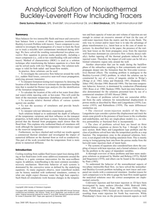
Solution Construction. Solution of the equation system defined in
Eqs. 1 through 3 and subject to the boundary and initial conditions
given in Fig. 1 is constructed by use of the method of character-
istics. The details of the solution of systems of equations arising in
multiphase transport in porous media is explained by Dindoruk
(1992) and Johns (1992). Solution of Eqs. 1 through 3 consists of
shocks, expansion waves, and zone of constant states. The full
solution is pieced together by use of those components subject to
a set of fractional-flow curves shown in Fig. 2. The fractional flow
shown in Fig. 2 is generated by use of the relative permeability
coefficients shown in Table 1 (Eqs. 10 and 11).
Fig. 1—Boundary and initial conditions (Riemann problem).
556 June 2008 SPE Reservoir Evaluation & Engineering
3. A sketch of the solution in a 2D state space (TD and g—as per
the transformation described in the Appendix) is shown in Fig. 3.
Addition of the tracer just lifts part of the solution path in the cD
dimension, as shown in Fig. 4. Figs. 3 and 4 show the behavior for
cold-water injection. For simplicity, we will start describing solu-
tion construction by use of Fig. 3:
• Solution starts with a leading shock from Initial Condition a
to Point b as dictated by the tangent drawn to the fractional-flow
curve for the reservoir (TסTi).
• Solution continues with an expansion wave from the Shock
Point b to the Equal Eigenvalue Point c, where g͑Sw͒ס
Ѩfw
ѨSw
ͯTD1ס
.
The solution of this equation will yield the upstream saturation
point (S*w) on the fractional-flow curve for the reservoir. This is
geometrically a tangent construction from (−, −␣) to the frac-
tional-flow curve of the reservoir.
• Next, the corresponding saturation point on the fractional-
flow curve of the injection point (well) needs to be determined.
This can be calculated by use of g͑S**w ͒ԽTD0ססg͑S*w͒ԽTD1ס. Because
S*w is already known from the previous step, S**w is the only un-
known in this equation, and it will give us the location of the
landing point (Point d) on the fractional-flow curve of the injection
point. In other words, this point is the point in which the interme-
diate eigenvalues of the two extreme temperatures are equal.
• Finally, the trailing segment of the solution will be from the
landing point on the fractional-flow curve of the injection point to
the inlet-contact discontinuity (Point e, 1−Sor with characteristic
speed of zero).
Additon of tracer “lifts” part of the solution path along the
concentration axis, as shown in Fig. 4. Because the tracer is a
noninteracting tracer, it will not impact the other variables, and the
location of the tracer can be obtained from
Ѩfw
ѨSw
ͯTD1ס
ס
fw
Sw
. Geo-
metrically, this is equivalent to drawing a tangent from the ini-
tial condition, (0,0), to the fractional-flow curve for the reservoir.
The difference between the cases without tracer vs. with tracer is
that the solution-path segment, (m–n), is in the third (concentra-
tion) dimension. Corresponding solution construction by use of
fractional-flow domain is shown in Fig. 1. Saturation profile in
terms of by use of eigenvalue segments is shown in Fig. 5.
The composition path is somewhat different for hot-water in-
jection. In that case, the composition path starts with a leading
shock from (Swc, 0) to the fractional-flow curve for the reservoir
and continues until the equal eigenvalue point on the fractional-
flow curve for the injection point (well). That point is defined by
drawing a tangent to the fractional-flow curve of the injection point
from (−,−␣). The equation for this tangent is g͑Sw͒ס
Ѩfw
ѨSw
ͯTD0ס
.
Again, the solution of this equation will yield the upstream satu-
ration point (S*w) on the fractional-flow curve for the fractional-
flow curve for the injection point. Next, the corresponding satu-
ration point on the fractional-flow curve of the reservoir (well) can
be determined by use of g͑S**w ͒|TD1ססg͑S*w͒|TD0ס. Again, S**w is the
only unknown in this equation. Then, the rest of the solution is the
same as that for the cold-water injection.
Corresponding solution construction by use of fractional-flow
domain is shown in Fig. 6. Saturation profiles in terms of use of
eigenvalue segments is shown in Fig. 7.
Sample Solutions. Analytical and numerical solutions are ob-
tained for both cold waterflooding and hot waterflooding. Numeri-
Fig. 3—Solution path in TD and g state space.
Fig. 4—Updated solution path in TD, g, and cD state space. a-b
-c-d-e path is for nonisothermal Buckley-Leverett without
tracer, and a-b-m-n-c-d-e path is for nonisothermal Buckley-
Leverett with tracer.
Fig. 2—Path construction on the fractional-flow curves for cold
waterflooding.
557June 2008 SPE Reservoir Evaluation & Engineering
4. cal solutions are obtained by use of a commercial simulator
(STARS Manual 2004). Input data are given in Tables 1 through 3.
Thermal properties and densities shown in Table 2 are used in
combination with the fractional-flow function shown below:
fw͑Sw, T͒ =
1
1 +
w
o
͑T͒
kro
krw
. . . . . . . . . . . . . . . . . . . . . . . . . . . . (10)
The fractional-flow function is a function of saturation resulting
from relative permeabilities and a function of temperature through
viscosities. The method described here, however, is general and
can take any combination of these dependencies (i.e., relative per-
meabilities as a function of temperature). For the solutions pre-
sented here, Corey-type relative permeabilities are used:
krw = krw
o
͑S͒nw
kro = kro
o
͑1 − S͒no
S =
Sw − Swr
1 − Sor − Swr
. . . . . . . . . . . . . . . . . . . . . . . . . . . . . . . . . . . . . (11)
The input parameters for the relative permeability functions are
shown in Table 1, and the fluid viscosities are shown in Table 3.
Cold Waterflooding. For this case, we have assumed injection
of cold water in which the oil viscosity increases within the tran-
sition zone behind the temperature front. For the example case
shown in Fig. 8, we have assumed 0.99-cp cold water displacing
2-cp oil, while oil viscosity increases to 8 cp behind the thermal
front. Solution starts from downstream to upstream with a Buck-
ley-Leverett-type shock front (a→b) on the fractional-flow func-
tion for the reservoir. Then it continues with an expansion wave
(b→c). The expansion wave on the fractional-flow function for the
reservoir is followed by a trailing shock (c→d), owing to tempera-
ture change. That shock is followed by a zone of constant state
(d→d), owing to the differences in the speeds of propagation be-
tween the trailing shock front and the expansion wave, (d→e), on
the fractional-flow curve for the injection point (well). As seen in
Fig. 8, the temperature front causes c→d shock and, as expected,
it is also aligned with it. The tracer shock, (m→n), does not in-
terfere with the structure of the temperature and saturation profiles.
The location of the tracer shock is a function of pore volumes
injected and the amount of initial water saturation within the tran-
sition zone. Tracer concentration moves slower than the leading
shock because of the absence of tracer in the initial water satura-
tion. One of the main observations that can be made is that the
temperature shock moves slower than the injected water front, and
Fig. 6—Path construction on the fractional-flow curves for
hot waterflooding.
Fig. 7—Solution-path construction by use of the eigenvalues for
hot waterflooding.
Fig. 5—Solution-path construction by use of the eigenvalues for
cold waterflooding.
558 June 2008 SPE Reservoir Evaluation & Engineering
5. the speed of propagation is a function of the thermal heat (mass)
capacity ratio (/␣) of the porous medium as well as the flow
properties of residing and invading fluids.
Although it is easy to solve the equation system posed by Eqs.
1 through 3 by use of a conservative fine-difference scheme (re-
sults not shown here), one of our main motivations is to implement
the assumptions cited here and solve the same/near-identical prob-
lem by use of a commercial simulator and compare the accuracy of
the solution. In Fig 8, we have used 1,000 gridblocks in the di-
rection of flow, and the numerical results agreed with the analyti-
cal results extremely well. Among all the dependent variables, the
tracer front exhibited a higher level of numerical dispersion (Lantz
1971) because of its self-sharpening nature, and it moved faster
than the temperature front. Resulting from the entry and exit to the
two-phase-flow region, the leading saturation shock did not exhibit
high levels of dispersion with respect to TD and cD fronts. Level of
numerical dispersion is a function of numerical Peclet number and
is a function of the derivative of the fractional-flow function
(Lantz 1971). Further discussion on numerical dispersion in the
context of 1D conservation equations can be found in Orr (2007).
Hot Waterflooding. For the hot-waterflooding case, we have
assumed injection of hot water in which the oil viscosity decreases
within the transition zone behind the thermal front. For the ex-
ample case shown in Fig. 9, we have assumed that 0.69-cp hot
water displacing 8-cp oil while oil viscosity decreases to 2 cp
behind the thermal front (Table 3). Corresponding solution con-
struction by use of fractional-flow domain is shown in Fig. 6.
Saturation profiles by use of eigenvalue segments are shown in
Fig. 7 Solution starts from downstream to upstream with a Buck-
ley-Leverett-type shock front (a→b) on the fractional-flow func-
tion for the reservoir. Then it continues with an expansion wave
(b→c). An expansion wave on the fractional-flow function for the
reservoir is followed by a zone of constant state (c→c) because the
landing point of the trailing shock, (c→d), on the fractional-flow
function for injection point (well) travels slower for the same
saturation. Again, the trailing shock, (c→d), is caused—and is
aligned—by the temperature shock. The tracer shock, (m→n),
does not interfere with the structure of the temperature and satu-
ration profiles. Similar to the cold-water-injection case, the loca-
tion of the tracer shock is a function of pore volumes injected and
the amount of initial water saturation within the transition zone.
Like the cold-water injection case, tracer concentration moves
slower than the leading shock because of the absence of tracer in
the initial water saturation. The temperature shock moves slower
than the injected water front, and the speed of propagation is a
function of the thermal heat (mass) capacity ratio, (/␣), of the
porous medium as well as the flow properties of the residing and
invading fluids.
The numerical solutions are also compared with the analytical
solution in Fig. 9 at tD52.0ס (pore volumes injected). In the
numerical solutions, 1,000 gridblocks are used in the direction of
flow, and the numerical results agreed with the analytical results
extremely well. Behavior of the numerical solution and the nu-
merical quality with respect to the analytical solution is the same
as the cold-waterflooding case and therefore will not be elaborated
once more.
Solution in Radial Coordinates. In reality, we are more inter-
ested in the radial-flow geometry than the linear geometry. Be-
cause the MOC solutions are similar, it is possible to perform a
simple coordinate transformation as defined by Welge (Welge et
al. 1962) and, later, by others in a more generalized form (Johns
and Dindoruk 1991; Johns 1992). The following dimensionless
variables will transform the solutions for linear geometry into ra-
dial coordinates without repeating the solution process:
rD =
r
L
. . . . . . . . . . . . . . . . . . . . . . . . . . . . . . . . . . . . . . . . . . . . . (12)
is for the radial distance, and
tD =
qt
L2
h
. . . . . . . . . . . . . . . . . . . . . . . . . . . . . . . . . . . . . . . . . (13)
is for the dimensionless time in radial coordinates. Here, L indi-
cates some characteristic distance in the radial domain. Therefore,
relabeling the linear distance xD as rD
2
(xD≡rD
2
) in Figs. 8 and 9
yields the analytical solutions for radial coordinates, as shown in
Figs. 10 and 11. In this case the dimensionless distance is equiva-
lent to the dimensionless radial distance squared. The comparative
details of radial vs. linear dimensionless variables are shown by
Johns (1992). Numerical implementation of the radial flow re-
quires a somewhat different approach, however. For that, the do-
main needs to be gridded appropriately by use of a radial-grid
system (Fig. 12). In addition, to capture the flow around the well
accurately, a logarithmically spaced grid system is needed. Nu-
merical solutions shown in Figs. 10 and 11 are generated by use of
1,000 grid cells. As in the case of linear geometry, the numerical
solutions agree well with the analytical solutions.
Numerical Experiments. In this section, we will focus on limited
numerical experiments to understand the impact of some of the
Fig. 9—Comparison of analytically constructed profiles for lin-
ear flow (method of characteristics) vs. numerical solution for
hot waterflooding at tD=0.25 pore volumes of injection. Nx=1,000
for the numerical solution.
Fig. 8—Comparison of analytically constructed profiles for lin-
ear flow (method of characteristics) vs. numerical solution for
cold waterflooding at tD=0.25 pore volumes of injection.
Nx=1,000 for the numerical solution.
559June 2008 SPE Reservoir Evaluation & Engineering
6. variables that we did not consider to set up the problem for the
analytical solutions.
Grid Sensitivity. For the sake of brevity, we will show only two
of the runs we have performed: fine- and coarse-grid runs. Fine-
grid runs are performed by use of 1,000 grids as before, and
coarse-grid runs are performed by use of 10 grids. In addition to
what we show here, we performed simulation runs with finer grids
(i.e., 10,000), and the results were similar to those shown here with
1,000 gridblocks. Comparison of the numerical results for both
cold-water and hot-water-injection cases are shown in Figs. 13
and 14. As can be seen in these figures, the temperature profile
and the tracer profiles are more prone to the numerical dispersion
than is the fluid saturation. In addition to the differences in the
numerical Peclet number (Lantz 1971), one of the reasons for
higher levels of dissipation of the temperature profile is that tem-
perature has more room to dissipate for all the phases and the rock,
and it is also a self-sharpening wave (Jeffery 1976).
Tracer dispersion is somewhat analogous to temperature; how-
ever, it moves faster and its dissipation is also related to the dis-
sipation of Sw because it resides in the water phase only. The
dissipation characteristics of the tracer front, however, are similar
to a semishock, in which one side of the shock resides on the
fractional-flow curve. In explicit solutions, dimensionless timestep
size must be less than dimensionless grid size for single-phase
flow and much less than grid size if the saturation derivative of the
fractional-flow function is greater than 1, as it will be for the
S-shaped fractional-flow curve appropriate to two-phase flow in a
porous medium, particularly when the injected fluid has a viscosity
that is less than that of the oil displaced. As a result, the effects of
numerical dispersion can be reduced by reducing grid size (and
therefore timestep size), but they cannot be eliminated entirely for
the finite-difference scheme. The limitation on timestep size is a
version of the Courant-Friedrichs-Lewy condition (Courant et al.
1967), which states that the finite-difference scheme of a simple
one-point explicit scheme is unstable if
p⌬tD
⌬xD
Ͼ1 for all equations
and characteristic speeds [p, eigenvalues (Orr 2007)].
Effect of Thermal Conduction/Overburden/Underburden Heat
Loss. Next, we have examined the impact of thermal conduction,
which had to be neglected to solve the system of equations ana-
lytically. The values used in the numerical investigation are given
in Table 4. The conductivity of underburden and overburden are
22.47 and 22.79 Btu/day-ft-ºF, respectively. The density and con-
ductivity products are 38.68 and 35.44 Btu/ft3
-ºF for overburden
and underburden, respectively.
Numerical results including the impact of thermal conduction
shown in Figs. 15 and 16 are obtained with Cartesian grids for
linear displacement. In the same figures, numerical solution with-
out the effects of conduction is also superimposed for comparison
purposes. Overall, the thermal front dissipates at tD.52.0ס The
location of the tracer front and the saturation front (and the profile)
do not change appreciably, however. In this study, the main focus
was the convection-dominant displacement, and a methodical ap-
proach to form benchmark solutions was presented for the solution
of saturation, temperature, and tracer equations. Although we did
not investigate the impact of heat conduction thoroughly, the im-
pact of heat conduction appears as significant on the basis of the
cases that we have considered for this work. Further work is
Fig. 11—Comparison of analytically constructed profiles for ra-
dial flow (method of characteristics) vs. numerical solution for
hot waterflooding at tD=0.25 pore volumes of injection. Nx=1,000
for the numerical solution.
Fig. 12—Well configuration and grid system used for the simu-
lation of radial-flow cases (Nr =1,000 by use of logarithmically
spaced grids).
Fig. 13—Numerical simulation of cold waterflooding with a
tracer by use of fine (Nx=1,000) and coarse (Nx=10) grids at
tD=0.25. Solid lines are the analytical solutions by use of the
method of characteristics.
Fig. 10—Comparison of analytically constructed profiles for ra-
dial flow (method of characteristics) vs. numerical solution for
cold waterflooding at tD=0.25 pore volumes of injection.
Nx=1,000 for the numerical solution.
560 June 2008 SPE Reservoir Evaluation & Engineering
7. needed to quantify the time scales that second-order effects (con-
duction, heat losses to underburden and overburden) make impor-
tant. Impact of conduction is discussed within the context of
steamflood by Prats (1985). Although the results are not shown
here, we have also included the effects of overburden and under-
burden heat losses. The inclusion of those effects did not change
the results significantly for the saturation and tracer profiles (for
the time scale considered). The temperature profile changed a
small amount, however.
Sensitivity to Rock/Fluid Thermal Properties. We have briefly
studied the impact of mass-based heat capacity of the rock and
fluid system. In this analysis, fractional-flow functions of the sys-
tem were not changed. The relevant parameters for the heat-
capacity sensitivity study are shown in Table 5. In Table 5, we
have tried to capture a wide range of realistic properties, but it is
possible to widen the ranges considered here even further. On the
basis of the scaling shown in Eq. 3, the thermal front will propa-
gate as dictated by the final values of ␣ and  as well as the
fractional-flow function of the system. Because the fractional flow
is kept the same in all cases, we can isolate the impact of ␣ and .
In all cases, the slow shocks seen in the saturation profiles corre-
spond to temperature shocks, and the temperature shock moves
significantly slower than the leading saturation front. The propa-
gation behavior of the thermal front is similar in the case of hot-
water injection. In fact, the speeds of the thermal fronts are the
same because we have considered the same fractional-flow curves,
as explained in the Sample Solutions section.
Between the parameters ␣ and ,  shows more variability with
respect to ␣ because of the contribution of the porosity term. It is
possible, therefore, to correlate the location of the temperature
front with respect to  alone for a given oil/water system. Because
finding the location of the temperature front can be obtained easily,
as explained in the Solution Construction section, by drawing a
tangent to the fractional-flow curve from (−, −␣), there is no need
to develop a generalized correlation for the speed of the tempera-
ture front. It is still possible, however, to see the speed of the
temperature front decrease as  increases (Fig. 17). Higher 
means that the proportion of the heat transferred to the rock is
higher, and, therefore, the temperature front will lag behind the
saturation front even more. In this figure, ␣ varied between 0.48
and 0.83 for the given set of fractional-flow function described by
the parameters given in Tables 2 and 3.
Conclusions
We have solved the nonisothermal Buckley-Leverett problem both
for hot- and cold-water injection including an inert tracer and
compared analytical solutions with numerical solutions. The pri-
mary conclusions are
1. Simplified analytical solution of the nonisothermal Buckley-
Leverett problem with tracer (both hot- and cold-water injec-
tion) is shown to be equivalent to three tangents drawn on the
fractional-flow function of the system.
2. The temperature front propagates much slower than the satura-
tion and tracer fronts and dissipates significantly when conduc-
tive terms are considered. The mobility changes induced by the
temperature front, therefore, cannot be mimicked in black-oil
simulators by modifying the mobility by use of the standard
interacting tracer options.
3. By use of the radial transformation of Welge (Welge et al.
1962), radial solutions are constructed. The temperature front
propagates (in distance) further in radial coordinates because of
quadratic dependence of the volume on radial distance.
4. The temperature front slows down as more heat is transferred to
the rock matrix (i.e., low porosity, high ).
5. Radial solution of the problem is compared with the numerical
solutions and shows the temperature front is more prone to
numerical dispersion.
6. Numerical solutions agree well with the analytical solutions.
Fig. 15—Numerical simulation of cold waterflooding with a
tracer by use of fine grids (Nx=1,000) at tD=0.25 including the
effects of conduction. Solid lines are the analytical solutions by
use of the method of characteristics.
Fig. 16—Numerical simulation of hot waterflooding with a tracer
by use of fine grids (Nx=1,000) at tD=0.25 including the effects of
conduction. Solid lines are the analytical solutions by use of the
method of characteristics.
Fig. 14—Numerical simulation of hot waterflooding with a tracer
by use of fine (Nx=1,000) and coarse (Nx=10) grids at tD=0.25.
Solid lines are the analytical solutions by use of the method of
characteristics.
561June 2008 SPE Reservoir Evaluation & Engineering
8. Nomenclature
a, b ס parameters for Langmuir-type adsorption function (Eq.
A-12)
A ס area open to flow, ft2
cD ס dimensionless tracer concentration
cDtD
ס partial derivative of dimensionless concentration with
respect to dimensionless time
cDxD
ס partial derivative of dimensionless concentration with
respect to dimensionless distance
ci ס injected tracer concentration, ppm
cvo ס heat capacity of oil, BTU/lbm-o
F
cvr ס heat capacity of rock, BTU/lbm-o
F
cvw ס heat capacity of water, BTU/lbm-o
F
D ס dimensionless adsorption term in Eq. A-13
DЈ ס adsorption term as described by Eq. A-12
fS ס partial derivative of fractional flow of water with
respect to water saturation, fS =
Ѩfw
ѨSw
fTD
ס partial derivative of fractional flow of water with
respect to dimensionless temperature, fTD
=
Ѩfw
ѨTD
fw ס fractional flow of water
g ס dimensionless ratio function defined by g=
fw+␣
Sw+
gtD
ס partial derivative of g with respect to dimensionless
time
gxD
ס partial derivative of g with respect to dimensionless
distance
h ס dimensionless ratio function defined by h=
fw
Sw
hЈ ס modified dimensionless ratio function defined by hЈ=
fw
Sw+
dD
dcD
.
I ס identity matrix
J ס coefficient matrix (Eq. A-1)
kro ס relative permeability of oil
ko
ro ס endpoint relative permeability of oil
krw ס relative permeability of water
ko
rw ס endpoint relative permeability of water
L ס distance, ft
no ס relative permeability exponent of oil
nw ס relative permeability exponent of water
Nr ס Number of grids in r-direction
Nx ס Number of grids in x-direction
q ס injection rate, ft3
/day
r ס radial distance, ft
rD ס dimensionless radial distance
S ס scaled water saturation defined by S=
Sw−Swr
1−Sor−Swr
, fraction
Sor ס residual oil saturation, fraction
StD
ס partial derivative of water saturation with respect to
dimensionless time
Sw ס water saturation, fraction
Sw,leadס water saturation of the leading (fast) shock, fraction
Swi ס initial water saturation, fraction
Swr ס residual water saturation, fraction
SxD
ס partial derivative of water saturation with respect to
dimensionless distance
Sw* ס water saturation obtained from g͑Sw͒=
Ѩfw
ѨSw
ͯTD=1
Sw** ס water saturation obtained from g͑S**w ͒|TD=0=g͑S*w͒|TD=1
t ס time, daysFig. 17—Characteristic propagation speed of TD front vs. .
562 June 2008 SPE Reservoir Evaluation & Engineering
9. tD ס dimensionless time
TD ס dimensionless temperature
TDtD
ס partial derivative of dimensionless temperature with
respect to dimensionless time
TDxD
ס partial derivative of dimensionless temperature with
respect to dimensionless distance
Ti ס initial (reservoir) temperature
Tw ס inner-boundary temperature
x ס linear distance
xD ס dimensionless distance
Xជ ס eigenvectors
␣ ס dimensionless property function defined by ␣=
ocvo
wcvw−ocvo
 ס dimensionless property function defined by
=
ocvo+
1−
rcvr
wcvw−ocvo
ס eigenvalues
o ס viscosity of oil, cp
w ס viscosity of water, cp
o ס density of oil, lbm/ft3
r ס density of rock, lbm/ft3
w ס density of water, lbm/ft3
ס porosity, fraction
Acknowledgment
Authors thank Shell E&P for granting permission to publish this
manuscript.
References
Barkve, T. 1989. The Riemann Problem for Nonstrictly Hyperbolic System
Modeling Nonisothermal, Two-Phase Flow in a Porous Medium. SIAM
J. of Applied Mathematics. 49 (3): 784–798. DOI: 10.1137/0149045.
Bratvold R. 1989. An Analytical Study of Reservoir Pressure Response
Following Cold Water Injection. PhD dissertation, Stanford, Califor-
nia: Stanford University.
Buckley, S.E. and Leverett, M.C. 1942. Mechanism of Fluid Displacement
in Sands. Trans., AIME 241: 107–116.
Courant, R., Friedrichs, K.O., and Lewy, H. 1967. On the Partial Differ-
ence Equations of Mathematical Physics. IBM J. of Research and De-
velopment Development 11 (2): 215–234.
Dindoruk, B. 1992. Analytical Theory of Multicomponent Multiphase Dis-
placement in Porous Media. PhD dissertation, Stanford, California:
Stanford University.
Fayers, F.J. 1962. Some Theoretical Results Concerning the Displacement
of a Viscous Oil by a Hot Fluid In a Porous Medium. J. of Fluid
Mechanics. 13: 65–76. DOI: 10.1017/S002211206200049X.
Hashem, M. 1990. Saturation Evaluation Following Water Flooding. En-
gineering thesis, Stanford, California: Stanford University.
Hovdan, M. 1989. Water Injection—Incompressible Analytical Solution
With Temperature Effects. Technical Report MH–1/86. In Norwegian.
Stavanger: Statoil.
Isaacson, E. 1980. Global Solution of a Riemann Problem for Non Strictly
Hyperbolic System of Conservation Laws Arising in Enhanced Oil
Recovery. New York City: The Rockefeller University.
Jeffery, A. 1976. Quasilinear Hyperbolic Systems and Waves. London:
Pitman Publishing.
Johns, R.T. 1992. Analytical Theory of Multicomponent Gas Drives With
Two-Phase Mass Transfer. PhD dissertation, Stanford, California:
Stanford University.
Johns, R.T. and Dindoruk, B. 1991. Theory of Three-Component, Two-
Phase Flow in Radial Systems. In Scale-Up of Miscible Flood Pro-
cesses. Final report, Contract No. DE-FG21-89MC26253-5, US DOE,
Washington, DC.
Lake, L. 1989. Enhanced Oil Recovery. Englewood Cliffs, New Jersey:
Prentice Hall.
Lantz, R.B. 1971. Quantitative Evaluation of Numerical Dispersion (Trun-
cation Error). SPEJ 11 (3): 315–320. SPE-2811-PA. DOI: 10.2118/
2811-PA.
Lauwerier, H.A. 1955. The Transport of Heat in an Oil Layer Caused by
Injection of Hot Fluid. Applied Science Research 5 (2–3): 145–150.
Marx, J.W. and Langenheim, R.H. 1959. Reservoir Heating by Hot Fluid
Injection. Trans., AIME 216: 312–315.
Myhill, N.A. and Stegemeier, G.L. 1978. Steam-Drive Correlation and
Prediction. JPT 30 (2): 173–182. SPE-5572-PA. DOI: 10.2118/5572-
PA.
Orr, F.M. Jr. 2007. Theory of Gas Injection Processes. Copenhagen, Den-
mark: Tie-Line Publications.
Platenkamp, R.J. 1985. Temperature Distribution Around Water Injectors:
Effects on Injection Performance. Paper SPE 13746 presented at SPE
Middle East Technical Conference and Exhibition, Bahrain, 11–14
March. DOI: 10.2118/13746-MS.
Pope, G.A. 1980. The Application of Fractional Flow Theory to Enhanced
Oil Recovery. SPEJ 20 (3): 191–205. SPE-7660-PA. DOI: 10.2118/
7660-PA.
Prats, M. 1985. Thermal Recovery. Monograph Series SPE, Richardson,
Texas, 7.
Roux, B., Sanyal, S.K., and Brown, S.L. 1980. An Improved Approach to
Estimating True Reservoir Temperature From Transient Temperature
Data. Paper SPE 8888 presented at the SPE California Regional Meet-
ing, Los Angeles, 9–11 April. DOI: 10.2118/8888-MS.
Rubinshtein, L.L. 1959. The Total Heat Losses in Injection of a Hot Liquid
Into a Stratum. Nefti Gaz 2 (9): 41–48.
Shutler, N.D. and Boberg, T.C. 1972. A One-Dimensional Analytical
Technique for Predicting Oil Recovery by Steam Flooding. SPEJ 12
(6): 489–498. SPE-2917-PA. DOI: 10.2118/2917-PA.
STARS Manual. 2004. Calgary: CMG.
Welge, H.J., Johnson, E.F., Hicks, A.L., and Brinkman, F.H. 1962. An
Analysis for Predicting the Performance of Cone-Shaped Reservoirs
Receiving Gas or Water Injection. JPT 14 (8): 894–898. SPE-294-PA.
DOI: 10.2118/294-PA.
Appendix
Eqs. 1 through 3 can be written in matrix form as:
΄
StD
TDtD
cDtD
΅+
΄
fs fTD
0
0 g 0
0 0 h
΅΄
SxD
TDxD
cDxD
΅=
΄
0
0
0
΅, . . . . . . . . . (A-1)
where h [water particle velocity as Isaacson (1980)] is defined by
h =
fw
Sw
. . . . . . . . . . . . . . . . . . . . . . . . . . . . . . . . . . . . . . . . . . . . (A-2)
This can also be rewritten symbolically as
͓I͔YជTD
− ͓J͔YជxD
= 0ជ, . . . . . . . . . . . . . . . . . . . . . . . . . . . . . . . . . (A-3)
where [I] is the identity matrix, [J] is the coefficient matrix, and Y
is the vector of dependent variables Sw, TD, and cD. The eigenvalue
problem posed by Eq. A-1 is
͓J − I͔Xជ = 0ជ. . . . . . . . . . . . . . . . . . . . . . . . . . . . . . . . . . . . . . . (A-4)
The eigenvalues for this system are
1 =
Ѩfw
ѨSw
, 2 = g, 3 =
fw
Sw
, . . . . . . . . . . . . . . . . . . . . . . . . . . . (A-5)
and the corresponding eigenvectors are
Xជ1 =
΄
1
0
0
΅, Xជ2 =
΄
Ѩfw
ѨSw
g −
Ѩfw
ѨTD
0
΅, Xជ3 =
΄
0
0
1
΅. . . . . . . . . . (A-6)
563June 2008 SPE Reservoir Evaluation & Engineering
10. Left eigenvectors can be extracted by use of
͓X1 X2 X3͔
΄
fs fTD
0
0 g 0
0 0 h
΅
−͓X1 X2 X3͔ = 0, . . . . . . . . . . . . . . . . . . . . . . . . . . . . . . . (A-7)
for 1=
Ѩfw
ѨSw
, yielding the left eigenvector
Xជ1 = ͫѨfw
ѨSw
− g,
Ѩfw
ѨTD
, 0ͬ. . . . . . . . . . . . . . . . . . . . . . . . . (A-8)
Multiplying both sides of Eq. A-1 with the left eigenvector de-
scribed by Eq. A-8 leads to new set of dependent variables de-
fined by
Ѩg
ѨtD
+ fs
Ѩg
ѨxD
= 0
ѨTD
ѨtD
+ g
ѨTD
ѨxD
= 0
ѨcD
ѨtD
+ h
ѨcD
ѨxD
= 0, . . . . . . . . . . . . . . . . . . . . . . . . . . . . . . . . . . . . (A-9)
or in matrix form,
΄
gtD
TDtD
cDtD
΅+
΄
fs 0 0
0 g 0
0 0 h
΅΄
gxD
TDxD
cDxD
΅=
΄
0
0
0
΅. . . . . . . . . . (A-10)
The differences between the new system of equations and the
system posed by Eq. A-1 are (1) a new dependent variable is
introduced in place of water saturation, (2) the coefficient matrix,
[J], is diagonal, and (3) the temperature derivative of the frac-
tional-flow function is not needed. The eigenvalues of the system
defined by Eq. A-10, however, are the same as the system defined
by Eq. A-1, and they are
1 =
Ѩfw
ѨSw
, 2 = g, 3 =
fw
Sw
. . . . . . . . . . . . . . . . . . . . . . . (A-11)
One of the main advantages of the new formulation originates
from the structure of the coefficient matrix [J]. The eigenvectors
defined by the eigenvalues are all constant. That means that g is
constant along constant TD, or TD is constant along constant g, and
similarly, cD lifts the solution only in the space defined by the
other two dependent variables (TD and g), as shown in Fig. 4.
Inclusion of noninteracting adsorption term for tracer transport
will not complicate the solutions or the equation system. Adsorption
can be represented by use of a Langmuir-type adsorption function:
DЈ =
ac
1 + bc
. . . . . . . . . . . . . . . . . . . . . . . . . . . . . . . . . . . . . . (A-12)
The transport equation for the tracer (Eq. 2) becomes:
Ѩ͑cDSw + D͒
ѨtD
+
Ѩ͑cD fw͒
ѨxD
= 0, . . . . . . . . . . . . . . . . . . . . . . . . . (A-13)
where D is the dimensionless adsorption function. Simplification
of Eq. A-13 will yield
ѨcD
ѨtD
+
ͫ fw
Sw +
dD
dcD
ͬѨcD
ѨxD
= 0, . . . . . . . . . . . . . . . . . . . . . . . (A-14)
hЈ =
fw
Sw +
dD
dcD
, . . . . . . . . . . . . . . . . . . . . . . . . . . . . . . . . . . . (A-15)
hЈ term is a modified version of the h term including a term related
to adsorption, as shown in Eq. A-9 and as defined by Eq. A-2.
In this case (the case with adsorption), the propagation speed of
the tracer can be obtained by drawing a tangent from (−h(0),0)
to the fractional-flow curve as explained in the section on solu-
tion construction.
SI Metric Conversion Factors
°F (°F−32)/1.8 ס °C
ft2
× 9.290 304* E−02 ס m2
ft3
× 2.831 685 E−02 ס m3
lbm × 4.535 924 E−01 ס kg
*Conversion factor is exact.
Deniz Sumnu-Dindoruk is a staff reservoir engineer and team
leader at Shell Exploration and Production Company, Uncon-
ventional Oil in Houston where she works in using unconven-
tional thermal recovery techniques to produce heavy oil and
bitumen reservoirs. She holds BS and MS degrees in petroleum
engineering from Middle East Technical University, Turkey and
a PhD degree in petroleum engineering from Stanford Univer-
sity. Birol Dindoruk is a principal technical expert in reservoir
engineering working for Shell International E&P since 1997, and
adjunct faculty at the University of Houston, department of
chemical engineering. He is a global consultant for fluid prop-
erties (PVT), miscible/immiscible gas injection, EOR and simu-
lation. Dindoruk holds a PhD degree in petroleum engineering
from Stanford University and an MBA degree from the Univer-
sity of Houston. He is a recipient of SPE Cedric K. Ferguson
Medal in 1994. Dindoruk was one of the Co-Executive Editors of
SPE Journal of Reservoir Evaluation and Engineering (2004–
2006) and is currently the Editor in Chief for Journal of Petro-
leum Engineering Science and Technology.
564 June 2008 SPE Reservoir Evaluation & Engineering