1. TIME SERIES ANALYSIS OF THE CORRELATION BETWEEN PROPERTY
INDEX RETURN AND OTHER ASSETS CLASS
LIANGKAI HU
 Data Description and preliminaryanalysis
I. Describe the time series character of NPI and FF data
1.
1) Required Statistics:
𝜇̂( 𝑁𝑃𝐼) =0.02260604
𝜎2̂(𝑁𝑃𝐼) = 0.0004631526
𝑄𝑢𝑎𝑛𝑡𝑖𝑙𝑒 𝑜𝑓 𝑁𝑃𝐼 𝐷𝑎𝑡𝑎:
0% 25% 50% 75% 100%
-0.0829 0.0175 0.0257 0.0336 0.0619
𝑄𝑢𝑎𝑛𝑡𝑖𝑙𝑒 𝑜𝑓 𝑆ℎ𝑎𝑟𝑝𝑒 𝑅𝑎𝑡𝑖𝑜 𝑐𝑎𝑙𝑐𝑢𝑙𝑎𝑡𝑒𝑑 𝑓𝑟𝑜𝑚 𝑁𝑃𝐼 𝑑𝑎𝑡𝑎:
0% 25% 50% 75% 100%
-4.6127508 0.1797810 0.8491328 1.3999694 2.9524901
2) Explanation of steps:
The formula used to calculate Sharpe Ratio is
𝑦𝑡 −𝑟 𝑓
𝜎(𝑦𝑡−𝑟 𝑓 )
, where 𝑦𝑡 is appraisal return, and
𝑟𝑓 is risk free rate. To calculate the standard deviation at year t, we need to use all the
data before time t. For accuracy purpose, we start at t=20. In this case, we can get 130
Sharpe ratios. Then we present the quantile of these 130 Sharpe ratio using R function
quantile().
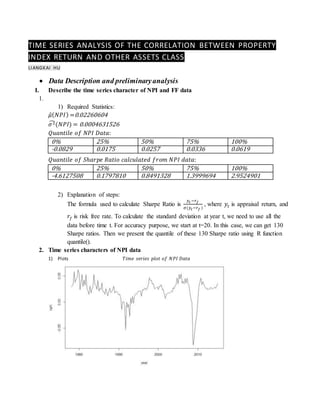
2. Time series characters of NPI data
1) Plots 𝑇𝑖𝑚𝑒 𝑠𝑒𝑟𝑖𝑒𝑠 𝑝𝑙𝑜𝑡 𝑜𝑓 𝑁𝑃𝐼 𝐷𝑎𝑡𝑎

2. 2) Trend: This time series does not present an obvious trend in mean level over time.
Seasonality: No, the time series does not have seasonality according to a seasonality test in R. (see the
explanation part for the test)
Other cyclic changes: From the graph, we can tell that there is not any other cyclicality either.
Irregular fluctuations and outliers: We can notice clearly from the graph that there are two outliers at
around 1992 and 2008 respectively. These two years are among the ones when the worst financial crisis
in history happened.
Variance over time: The variance seems stable over time.
Stationarity: According to the Augmented Dicky Fuller Test, this time series is stationary.
ACF & PACF:
By observing these two plot, we can get potential candidate model AR(3),AR(5),AR(7).

3. 3. Time series characters of FF Rm-Rf series
𝑇𝑖𝑚𝑒 𝑠𝑒𝑟𝑖𝑒𝑠 𝑝𝑙𝑜𝑡 𝑜𝑓 𝑅𝑚 − 𝑅𝑓
Characteristics: No obvious trend, no seasonality, no other long term cyclic changes,
Variance stable over time, no significant outliers.
𝑇𝑖𝑚𝑒 𝑠𝑒𝑟𝑖𝑒𝑠 𝑝𝑙𝑜𝑡 𝑜𝑓 𝑆𝑀𝐵 𝑡𝑖𝑚𝑒 𝑠𝑒𝑟𝑖𝑒𝑠

4. Characteristics: No obvious trend, no seasonality, no other long term cyclic changes,
Variance stable over time, no significant outliers.
𝑇𝑖𝑚𝑒 𝑠𝑒𝑟𝑖𝑒𝑠 𝑝𝑙𝑜𝑡 𝑜𝑓 𝐻𝑀𝐿 𝑡𝑖𝑚𝑒 𝑠𝑒𝑟𝑖𝑒𝑠
Characteristics: No obvious trend, no seasonality, no other long term cyclic changes,
Variance stable over time, significant outliers around year 2000.
II. Unsmooth the NPI data
1. Why NPI data has high autocorrelation parameters and the harm of using NPI data
without unsmooth procedures?
Answer: According to Fisher et al (1994), due to the nature of infrequent transaction in real
estate market, very little appraisal information is available to update the NPI data. Thus, although
NPI data is reported quarterly, it is actually only partially updated, with many past appraised
values being reported as the present value. This explains why NPI data are highly auto-
correlated. This inertia of change in NPI data results in underestimated risk in real estate
investment (Marcato & Key 2007), which is the main cause of the discrepancy between the
weights of real estate in theoretical portfolios and practical ones.
2. Use Autoregressive model to unsmooth the NPI data, including AR(1), AR(1,4) and selected
AR(p) model.
1) AR(1)
Coefficients:

5. ar1
0.8965
Quantiles of unsmooth returns:
0% 25% 50% 75% 100%
-0.78591494 -0.03241801 0.02879735 0.08621801 0.45856443
Goodness of fit:
Box-Ljung test
Lag 10 15 20
P-value 1.259e-10 3.593e-09 9.436e-08
Conclusion: AR(1) model fails the Box-Ljung test, indicating that it is not an adequate
model.
Method used: Run arima(1,0,0) in R to fit the NPI data. (Note: I used include.mean = FALSE
statement to force out intercept terms.) Get the coefficient and treat it as 𝑤1, calculate 𝑤0by
using 𝑤0 = 1 − 𝑤1. Then unsmooth return equal to the residuals vector of the fitted model
divided by 𝑤0 .
2) AR(1,4)
Coefficients:
ar1 ar4
0.74868672 0.05411907
Quantiles of unsmooth returns:
0% 25% 50% 75% 100%
-0.42275307
(-42.28%)
-0.00336876
(-0.34%)
0.02608784
(2.61%)
0.05304100
(5.30%)
0.20070541
(20.07%)
Goodness of fit:
Box-Ljung test
Lag 10 15 20
P-value 4.772e-07 6.534e-06 8.767e-05
Conclusion: AR(1,4) model fails the Box-Ljung test, indicating that it is not an adequate
model.
Method used: First I removed the mean from the appraisal return series. Then I used FitARp
function in package FitAR to fit the subset autoregressive model. When calculating economic
returns, I added back the mean. The rest are similar to the steps discussed above. Calculating
𝑤̂0 by setting 𝑤0̂ = 1 − 𝑤1̂ − 𝑤2̂.

6. 3) AR(p) model
𝐵𝐼𝐶 𝑜𝑓 𝐴𝑅(1) 𝑡𝑜 𝐴𝑅(20) 𝑚𝑜𝑑𝑒𝑙
Selective p: 𝑝 = 7 (Because AR(7) has smallest BIC value)
Coefficients:
ar1 ar2 ar3 ar4 ar5 ar6 ar7
0.7789 0.2874 -0.2037 0.3953 -0.4716 -0.1411 0.2907
Quantiles of unsmooth returns:
0% 25% 50% 75% 100%
-1.24620194 -0.05936834 0.03307686 0.09563076 0.51294472
Goodness of fit:
Box-Ljung test
Lag 10 15 20
P-value 0.1649 0.4509 0.8124
Conclusion: AR(7) model passed the Box-Ljung test, indicating that it is an adequate model.
Method used: first fit the NPI data using AR(1) to AR(20) models by running a for loop, then
selecting the best among them by choosing the one with smallest BIC value. The process of
estimating the unsmooth return is the same as above.
3. Use selectedMA(q) process to unsmooth data.
Selected q: 𝑞 = 8 (Because MA(8) model has smallest BIC value)

7. 𝐵𝐼𝐶 𝑜𝑓 𝐴𝑅(1) 𝑡𝑜 𝐴𝑅(20) 𝑚𝑜𝑑𝑒𝑙
Coefficients:
ma1 ma2 ma3 ma4 ma5 ma6 ma7 ma8
0.7757 0.919 0.8185 1.1036 0.6995 0.4699 0.2618 0.2679
Quantiles of unsmooth returns:
0% 25% 50% 75% 100%
-0.46864828 -0.01167132 0.02629124 0.05668086 0.19842841
Goodness of fit:
Box-Ljung test
Lag 10 15 20
P-value 0.2374 0.7008 0.9525
Conclusion: MA(8) model passed the Box-Ljung test, indicating that it is an adequate model.
Methods used: similarly to the model selection process of AR(p) model, we first run a for loop to
fit NPI data into MA(1) to MA(20) models. Then we select the best among them by choosing the one
with smallest BIC value. To calculate the unsmooth return, we first estimate c by setting 𝑐 = 1 +

8. ∑ 𝜃𝑖
8
𝑖=1 , i.e. c equals to the sum of all coefficients of the fitted MA(8) model plus 1. Then the unsmooth
return is the residuals of the fitted model times c.
4. Calculate the Sharpe ratio sequence for MA(8) unsmooth return
1) Volatility of unsmooth series
𝜎̂( 𝑢𝑛𝑠𝑚𝑜𝑜𝑡ℎ 𝑠𝑒𝑟𝑖𝑒𝑠) =0.07315946
𝜎2̂( 𝑢𝑛𝑠𝑚𝑜𝑜𝑡ℎ 𝑠𝑒𝑟𝑖𝑒𝑠) = 0.0053523
Quantile of ongoing Volatility of unsmooth series
0% 25% 50% 75% 100%
0.06104052 0.06504899 0.07030149 0.07542984 0.08655517
Method used: Ongoing volatility at time t is calculated using data from time 1 to time t.
Notice the first 20 data has been truncated to maintain the accuracy of volatility.
2) Quantile of Sharp ratio of unsmooth series
0% 25% 50% 75% 100%
-6.2948034 -0.3173747 0.2255852 0.6258938 2.5409855
Method used: Used exactly the same methods used in first question.
3) Discuss the result
Answer: We notice that there is a significance increase in variance from NPI return to
unsmooth return. (Variance of NPI data is estimated to be 0.0004631526, variance of
unsmooth return is estimated to be 0.0053523.) This increase is due to introduce of the
random terms (white noise variables) into the model.
III. Factor Loading Estimation
1. FF model for NPI data
1) Compound monthly data to quarterly data
Quantile of quarterly compounded FF factors
Rm-Rf 0% 25% 50% 75% 100%
-0.24383062 -0.02446885 0.03096875 0.06801565 0.20666690
SMB 0% 25% 50% 75% 100%
-0.105394419 -0.023295836 0.003485358 0.037692092 0.127225054
HML 0% 25% 50% 75% 100%
-0.190585458 -0.030507828 0.005510618 0.033275884 0.249860759
Method used: I used Excel to compound monthly return to quarterly return using the
formula provided in lecture notes: 𝑓𝑞𝑢𝑎𝑟𝑡𝑒𝑟𝑙𝑦 = (1 + 𝑓𝑡)(1 + 𝑓𝑡−1)(1 + 𝑓𝑡−2) − 1.
2) Fit the FF three factors to NPI return

9. Regression Coefficient
Intercept RmRf SMB HML
Coefficient 0.00994 0.03410 -0.03639 0.02115
p-value 1.4e-07 0.152 0.355 0.484
Significance? Yes No No No
Significance test shows that FF factors do not fit well to the original NPI return data,
suggesting that certain unsmooth process is necessary.
2. Estimate factor loading via unsmooth data
1) AR(1,4) model
i) Regression Coefficient
Intercept RmRf SMB HML
Coefficient 0.005707 0.169476 0.006780 0.193464
p-value 0.3269 0.0285 0.9574 0.0490
Significance? No Yes No Yes
Significance test shows that FF models fits better to unsmooth returns using Fisher
model compared to original NPI returns.
ii) Model adequacy test:
Firstly, we check R-squared and adjusted R-squared value. Higher value often implies
the adequacy of model.
Secondly, we check normal QQ-plot to check the normality assumption of the residuals
and Durbin-Watson test to examine whether there exists autocorrelations in residuals.
Result:
• R-squared
Multiple R-squared: 0.04899
Adjusted R-squared: 0.02931
Note: R-squared is too small to show the model is adequate.
• Normal QQ-plot
We notice that the residuals are heavy-tailed. This indicates the poor fit of the model.
• Durbin-Watson Test
D-W Statistics 2.260885
p-value 0.116

10. Thus we do not reject 𝐻0 , i.e. error terms are not correlated. Thus D-W test shows the
residuals are not auto-correlated.
MA(8) model
Regression Coefficient
Intercept RmRf SMB HML
Coefficient 0.004615 0.212477 0.043366 0.241563
p-value 0.4570 0.0103 0.7488 0.0215
Significance? No Yes No Yes
Significance test shows similar result as in AR(1,4) model.
Model adequacy test:
Result:
• R-squared
Multiple R-squared: 0.07021
Adjusted R-squared: 0.05097
Note: R-squared is too small to show the model is adequate.
• Normal QQ-Plot
We notice that the residuals are heavy-tailed. This indicates the poor fit of the model.
• Durbin-Watson Test
D-W Statistics 2.309212
p-value 0.068
Thus we do not reject 𝐻0 , i.e. error terms are not correlated. Thus D-W test shows the
residuals are not auto-correlated.

11. 3. Estimate factor loading via PICMO model (Use MA(8) model to carry out this
approach)
1) Briefly state PIMCO approach
Answer: By Dimson Model, we have 𝑦𝑡 = 𝑤0 𝑟𝑡 + 𝑤1 𝑟𝑡−1 + ⋯+ 𝑤 𝑞 𝑟𝑡−𝑞 (1)
In factor loading, we have 𝑟𝑡 − 𝑟𝑓 = 𝛼 + ∑𝛽𝑖 𝑓𝑖,𝑡 + 𝑒 𝑡 (2)
By substituting (2) into (1), we have
𝑦𝑡 = 𝑤0(𝑟𝑓 + 𝛼 + ∑𝛽𝑖 𝑓𝑖,𝑡 + 𝑒 𝑡) + ⋯+ 𝑤 𝑞 (𝑟𝑓 + 𝛼 + ∑𝛽𝑖 𝑓𝑖,𝑡−𝑞 + 𝑒 𝑡−𝑞)
= (𝑤0 + ⋯+ 𝑤 𝑞)(𝑟𝑓 + 𝛼) + ∑ 𝛽𝑗
𝑘
𝑗=1
∑ 𝑤𝑖 𝑓𝑡,𝑗−𝑖
𝑚
𝑖=1⏟
𝑋 𝑗,𝑡
+ (𝑤0 𝑒 𝑡 + ⋯+ 𝑤 𝑞 𝑒𝑡−𝑞)⏟
𝜀 𝑡
= 𝑟𝑓 + 𝛼 + ∑ 𝛽𝑗
𝑘
𝑗=1
𝑋𝑗,𝑡 + 𝜀𝑡
𝑇ℎ𝑒𝑟𝑒𝑓𝑜𝑟𝑒, 𝑤𝑒 𝑔𝑒𝑡
𝑦𝑡 − 𝑟𝑓 = 𝛼 + ∑ 𝛽𝑗
𝑘
𝑗=1
𝑋𝑗,𝑡 + 𝜀𝑡
Thus we need to first convert 𝑓𝑗 to 𝑋𝑗 using 𝑤𝑖, 𝑖 = 0 … 𝑚 as weight. Then we run
regression of unsmooth return minus risk free return against 𝑋𝑗, 𝑗 = 1,2,3 to get factor
loadings (𝛽1, 𝛽2, 𝛽3).
2) State w sequence used in this model.
( 𝑤0, 𝑤1, 𝑤2, 𝑤3, 𝑤4, 𝑤5 , 𝑤6, 𝑤7, 𝑤8) = (0.158, 0.123, 0.146, 0.130, 0.175, 0.111, 0.074,
0.041, 0.042)
Method used: 𝑤𝑖 =
𝑐𝑜𝑒𝑓𝑓[ 𝑖]
𝑐
𝑓𝑜𝑟 𝑖 = 1 … 8, where 𝑖 is the 𝑖 𝑡ℎ
coefficient of MA(8)
model, and 𝑤0 = 1 − 𝑤1 − ⋯− 𝑤8 .
3) Provide the quantile for 𝑿𝒋,𝒕
0% 25% 50% 75% 100%
𝑋1,𝑡 -0.078805273 0.007951135 0.023720593 0.041767578 0.066358751
𝑋2,𝑡 -0.047188881 -0.007717033 0.003338804 0.018847205 0.038861845
𝑋3,𝑡 -0.059796106 -0.003581999 0.008348817 0.021353808 0.079524067
Methods used: I first created a vector 𝑋 = (𝑋1, 𝑋2, 𝑋3), where 𝑋𝑖 is a vector of 130
components. Then I used a double for loop to calculate each value of 𝑋𝑖, using the
formula: 𝑋𝑗,𝑡 = ∑ 𝑤𝑖 𝑓𝑗,𝑡−𝑖, ∀𝑗8
𝑖=1 .

12. 4) Provide the model coefficients of the model and discuss the significance of the
coefficients.
Regression Coefficients
Intercept 𝑋1,𝑡 𝑋2,𝑡 𝑋3,𝑡
Coefficient -0.002355 0.450366 0.204699 0.261274
p-value 0.247631 4.01e-14 0.020543 0.000142
Significance? No Yes Yes Yes
Significance test shows that PIMCO methods fits much better than models discussed
before.
Method used: fit a linear model of appraisal return minus risk free rate against three FF
factors.
5) Discuss model adequacy
Answer:
• R-squared
Multiple R-squared: 0.3587
Adjusted R-squared: 0.3447
Note: R-squared is too small to show the model is adequate.
• Normal QQ-Plot
The residuals are a little left-skewed, indicating the poor fit of the model.
• Durbin-Watson Test
D-W Statistics 0.6793314
p-value 0
Thus we reject 𝐻0 ,i.e. error terms are correlated. Thus D-W test shows the model is not
adequate.

13. 6) Discuss your result
Answer: We notice that directly regressing NPI returns against FF factors results in the
worst fit (low significance of coefficients), while regressing using Pimco’s method
provides the best fit in the sense of coefficients significance. This fact may be stemmed
from the high auto-correlation among NPI returns. The unsmooth process has reduced
the autocorrelation in some sense. However, an interesting phenomenon is that
unsmoothing using AR(1,4) model and MA(8) model result in similar goodness of fit.
This collaborates the point of view raised by Marcato and Key that “model selection has
little effect on asset allocation choices”.
Reference:
1. FISHER et al. (1994). Value Indices of Commercial Real Estate: A Comparison of Index
Construction Methods. Journal of Real Estate Finance and Economic, 9, 137–164.
2. Marcato, G., & Key, T. (2007). Smoothing and Implications for Asset Allocation Choices. The
Journal of Portfolio Management, 33(5), 85–99.