Case 2

Introduction
In this case, 16 stocks were selected to find out the minimum variance portfolio. Hang
Seng Industry Classification System would be a good tool to select stocks according to their
different industries, it is a system designed for the Hong Kong Stock market, covering 11
industries and 28 sectors.
4 stocks from materials industry, 3 stocks from industrial Goods industry, 3 stocks from
the Consumer Services industry and 4 stocks from the Properties and Construction industry were
selected to form a portfolio in order to determine the minimum variance of the portfolio.
For a minimum variance portfolio, it is a portfolio where the investor invest their money
to buy the stocks according to the portfolio weights of different selected stocks, at which the
investor is in the lowest risk situation when compare to other portfolio weights of the same group
of stocks.
Methodology
` First, to compute the minimum variance portfolio, some basic information are needed,
using Bloomberg, the end-of-month closing price from February 2012 to February 2104 of the
selected stocks could obtained.
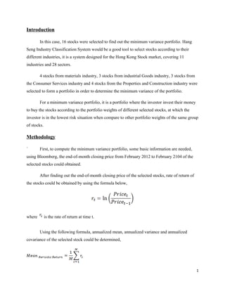
After finding out the end-of-month closing price of the selected stocks, rate of return of
the stocks could be obtained by using the formula below,
where is the rate of return at time t.
Using the following formula, annualized mean, annualized variance and annualized
covariance of the selected stock could be determined,
1

where is the rate of return at time t, M is the total number of period , n is the number of
period per year.
After finding the annualized mean, variance and covariance, the annualized mean vector
and the covariance matrix of the rate of return could be obtained, where the annualized mean
vector of rate of return is in the form as below,
where is the annualized mean of rate of return of the stock.
The form of the covariance matrix of the rate of return of the selected stocks is shown below,
2

where is the covariance of the stock rate of return and the rate of return, if
i = j, then represents the variance of the stock rate of return.
By the Markowitz portfolio theory, which developed by Harry Markowitz, who derived
the expected rate of return for a portfolio of assets and an expected risk measure. This model
shower that the variance of the rate of return was a meaningful measure of portfolio risk under a
reasonable set of assumptions. This model derived the formulas for computing the variance of a
portfolio not only indicated the importance of diversifying the investments to reduce the total
risk of a portfolio, but also showed how to effectively diversify. The Markowitz solution can be
found by using the method of Lagrange Multiplier, then the minimum variance set of the
portfolio could be determined, where the minimum variance set would be shown as below,
where represents the portfolio weight of the stock.
The mean ) and standard deviation ( ) of the annual rate of return of this minimum
variance portfolio then could be calculated
.
3

Then the mean-standard deviation diagram could be computed when setting two different
level of expected rate of return, which contained the minimum variance set, finally the efficient
portfolio with minimum variance could be determined.
In the above case, only one constraint exist, which is the sum of the 16 portfolio weights
(wi) need to equal to one. Now adding one more constraint to the Lagrange Multiplier, setting the
expected rate of return of the portfolio equal to the second highest annual rate of return among
16 selected stocks, which means adding the following constraints,
Using the two fund theorem, the weights of different selected stocks then could be calculated
where w1i represents the weightings of the ith
stock in the portfolio 1, w2i is the weightings of the
ith
stock in the portfolio 2
4

Select 16 stocks in 4 given industries
Using the Hang Seng Industry Classification system, the 16 stocks were selected as
follow,
Materials Stock Code
1 297 Sinofert
2 347 Angang Steel
3 1208 MMG
Inductrial Goods
1 148 Kingboard Chem
2 316 OOIL
3 566 Hanergy Solar
4 658 C Transmission
Consumer Services
1 66 MTR Corporation
2 293 Cathay Pac. Air
3 308 China Travel HK
4 753 Air China
5 69 Shangri-La Asia
Properties & Construction
1 1 Cheung Kong
2 12 Henderson Road
3 17 New World Dev
4 119 Poly Property
5

Find the end-of-month closing price
The end-of-price of the 16 selected stocks from February 2012 to February 2014 were
attached in the Appendix A.
Annualized mean vector and covariance matrix
By using the formula stated in the methodology part, the annualized mean vector of the
annual rate of return can be calculated and the result is shown below,
The covariance matrix can also be computed according to the formula below,
where M represents the total number of period, n represents the number of period per year.
6

The covariance matrix of the annual rate of return of these 16 selected stocks was attached in the
Appendix B.
Find the minimum variance set and the mean-standard deviation
diagram
To find out the minimum variance set, two set of solution that have the minimum
variance with different level of expected return need to be considered as to apply the two fund
theorem.
Setting the two expected return as 0.002 and 0.1, two different set of solutions including
the weightings of each of the 16 selected stocks, the portfolio mean and standard deviation of the
rate of return could be obtained by using the Langrage Multiplier and the formula stated above.
In this case, rather than one constraint, two constraints were subjected to minimize the
variance of the portfolio,
where in this case would equal to 0.002 and 0.1 respectively in order to find out two set of
solutions according to the different expected rate of return.
7

Find out and then put them equal to zero, there would have 18 equations and 18
unknowns, after that, transformed the 18 equations into the form ,
V is the var-cov(r) matrix
8

R is the annualized mean vector,
Result could be computed and the solutions of the two portfolios with different expected rate of
return could be found in the Appendix C.
Two sets of solution could be computed, using the result of the weightings of the 26
selected stocks in two different expected rate of return, the mean and standard deviation of the
portfolio could be obtained, letting the portfolio with expected rate of return 0.002 be portfolio A
and the one with expected rate of return 0.1 be portfolio B, the table below could be constructed,
portfolio A portfolio B
variance 0.007930757 0.008376584
S.D 0.089054796 0.091523679
expected rate of
return
0.002 0.1
covariance 0.00786807
where the covariance is computed using the equation below,
XA is the matrix of weightings of the 16 selected stocks in portfolio A, XB represented that of
portfolio B. V is the variance covariance matrix of the rate of return of the 16 selected stocks.
9

Consider portfolio A as asset A and portfolio B as asset B, then using the two assets case,
the minimum variance set can be calculated and the diagram could be computed. Let
and be the rate of return of the asset A and B respectively, has the mean of and the
variance of ; has the mean and variance of and respectively. The covariance of
and is .
Let x and 1-x be the portfolio weight of asset A and asset B respectively. The rate of
return of the portfolio and the mean of the rate of return are,
and the variance is,
Different portfolio weights involving the two portfolios mentioned above are used with the mean
and standard deviation of the rate of return of portfolios that are listed in the following table,
weight of portfolio A portfolio standard deviation portfolio mean
-0.5 0.095015251 0.149
-0.4 0.094206088 0.1392
-0.3 0.093451058 0.1294
-0.2 0.092751482 0.1196
-0.1 0.092108624 0.1098
0 0.091523679 0.1
0.1 0.090997764 0.0902
0.2 0.090531908 0.0804
0.3 0.090127041 0.0706
0.4 0.08978399 0.0608
0.5 0.089503464 0.051
0.6 0.089286054 0.0412
10

0.7 0.089132221 0.0314
0.8 0.089042294 0.0216
0.9 0.089016467 0.0118
1 0.089054796 0.002
1.1 0.089157199 -0.0078
1.2 0.089323455 -0.0176
1.3 0.089553207 -0.0274
1.4 0.08984597 -0.0372
1.5 0.09020113 -0.047
After finding the portfolio standard deviation and mean with different weighting of portfolio A
and B, the mean-standard deviation diagram could be obtained by the minimum variance sets in
the table above,
From the diagram above, the minimum-variance set has bullet shape, there is a special
point having the minimum variance which called minimum-variance point, which is shown by
the cross in the above diagram. Using this minimum-variance point, the efficient portfolio could
be obtained by using the two fund theorem.
11

The curve in the above mean-standard deviation diagram defined by nonnegative
mixtures of two assets A and B lies within the triangular region shown below which defined by
the two original assets A and B and point on the vertical axis of height is
Point on the vertical axis of height:
By substituting the value of , the vertical axis of height is 0.05033
Using the two fund theorem,
By solving the equation, x = 0.50684 and using the equation stated before, the efficient portfolio
could be calculated easily, the mean, variance and standard deviation of the portfolio could also
be found out, the mean of this portfolio is equal to 0.05033 and the variance is 0.008008.
12

Stock Allocation
Sinofert -0.00612
Angang Steel -0.137344
MMG 0.1544809
Kingboard Chem -0.199923
OOIL -0.088097
Hanergy Solar 0.0077333
C Transmission 0.0806506
MTR Corporation 0.6629117
Cathay Pac. Air 0.1650581
China Travel HK 0.3799111
Air China 0.0911574
Shangri-La Asia -0.150657
Cheung Kong 0.289253
Henderson Road 0.1659749
New World Dev -0.378129
Poly Property -0.036862
expected rate of return 0.05033
Variance 0.0080078
Determine the efficient portfolio
To find the solution of the Markowitz model, Lagrange Multiplier is a good method to
solve this problem, by setting the condition and the constraints,
where wi is the portfolio weight of the ith
stock of the 16 selected stocks.
13

Then using the method of Lagrange Multiplier, the equation below could be obtained,
After setting the equation above, by finding and , then put these 17 equations equal to
zero,
where i=1,2,3,….,16
Using as an example, it can be used to prove the 17 equations can be expressed in a matrix
form.
which is the same as
14

For i=1,2,3,…16, same expression could be obtained. When combining these 16 equation to
matrix form like the one above, the below result would be obtained,
Also, for the , could also be transformed to matrix form
By combing all the matrix above, the matrix form of these 17 equations were shown as below,
V is the var-cov(r) matrix
15

is in the form of , where
By using the property of matrix, value of matrix x could be found out easily,
By using the var-cov(r) matrix obtained above, the weightings of the 16 selected stocks with the
minimum variance could be found out eventually, the result was shown below,
16

The mean and the standard deviation of the portfolio can be calculated using the formula stated
in the methodology part,
.
The mean and variance of the annual rates of return of this minimum variance set is 0.01276 and
0.0079739 respectively.
17

Stock Allocation
Sinofert 0.0182314
MMG 0.1938072
OOIL -0.091607
Hanergy Solar -0.00247
Air China 0.0542938
Variance 0.0079239
The efficient portfolio can also be estimated by the mean-standard deviation diagram
shown above. For the diagram above, the minimum-variance point is (0.089016467, 0.0118),
which means the expected rate of return and standard deviation of the efficient portfolio is
0.0118 and 0.089016467 respectively. At this level of mean, by checking the table in the
previous page, the weight of portfolio A is 0.9, which means x=0.9, by the two-fund theorem,
two efficient funds can be established so that any efficient portfolio can be duplicated, in terms
of mean and variance, as a combination of these two. On other words, all investor seeking
efficient portfolios need only in combinations of these two funds.
is the weighting of the ith
stock of the 16 selected stocks in the efficient portfolio,
and are weightings of the ith
stock of the selected stocks in the portfolio A and portfolio
B which have found already in the previous part.
18

The efficient portfolio would be,
with the mean equal to 0.118 and variance equal to 0.0079239 which used the annualized mean
vector and the variance-covariance matrix of the rate of return to compute.
Find the efficient portfolio when given the target expected rate of
return
This time setting the target expected rate of return as the 2nd
highest annualized mean of
rate of return of the 16 selected stocks, by using the same method as before, the efficient
portfolio could be calculated easily,
By checking the annualized mean vector of the rate of return of the selected stocks, the
target expected rate of return is 0.03491, using two fund theorem,
19

Then the weightings of the stocks in this efficient portfolio are,
Stock Allocation
Sinofert 0.0038748
MMG 0.170622
OOIL -0.089537
Air China 0.0760271
Variance 0.0159061
the portfolio mean and variance are 0.0349078 and 0.0159061 respectively.
Conclusion
From the result calculated above, a portfolio which consists of a basket of stocks has the
lowest variance compare to any single stock in the basket. In the case above, the portfolio
consists of the 16 selected stocks can construct a efficient minimum variance portfolio has a
relatively lower variance when compare to the 16 stocks, which means the portfolio would have
a lower risk for investor to invest comparing to the singe stocks. Moreover, when more and more
stocks are added into the portfolio, the variance of the minimum efficient portfolio would be
lower and lower, the more the stocks in the portfolio, the lower the variance, which implied a
lower risk could be obtained. This phenomenon called diversification. Investor always pretend to
invest in an assets which has a lower risks, which mean a relatively lower variance portfolio, by
20

diversification, choosing a portfolio is a better choice than buying any one of the selected stocks
in the portfolio individually.
Appendix
Appendix A.
End-of-month stock price of the 16 selected stocks.
Materials
Month Price Ln((St)/(St-1)) Price Ln(St/St-1) Price Ln(St/St-1)
Feb-12 2.31 6.04 4.45
Mar-12 1.89 -0.200670695 4.99 -0.190968102 3.74 -0.173818485
Apr-12 1.69 -0.1118483 5.31 0.062155925 3.96 0.057158414
May-12 1.34 -0.232058915 4.45 -0.176687739 3.33 -0.173271721
Jun-12 1.19 -0.118716307 4.22 -0.053068968 3.23 -0.030490167
Jul-12 1.58 0.28347154 4 -0.053540767 2.94 -0.094072556
Aug-12 1.49 -0.058648727 3.79 -0.053928342 2.89 -0.017153079
Sep-12 1.52 0.019934215 4 0.053928342 2.97 0.027305451
Oct-12 1.64 0.075985907 4.65 0.150572858 3.08 0.036367644
Nov-12 1.65 0.006079046 4.88 0.048278 3.02 -0.019672766
Dec-12 1.88 0.130496489 5.68 0.151806013 3.21 0.061014106
Jan-13 1.93 0.026248226 5.74 0.010507978 3.14 -0.022048137
Feb-13 1.92 -0.005194817 5.22 -0.094961808 3.43 0.088337461
Mar-13 1.97 0.025708357 4.25 -0.205578419 2.85 -0.185241267
Apr-13 1.68 -0.159239749 4.57 0.072594222 2.33 -0.201450727
May-13 1.78 0.057819571 4.22 -0.079678077 2.14 -0.085062439
Jun-13 1.3 -0.3142491 3.81 -0.102205939 2.03 -0.052770036
Jul-13 1.21 -0.071743905 4.3 0.120985834 1.87 -0.082097362
Aug-13 1.21 0 4.88 0.126530197 1.75 -0.066322643
Sep-13 1.29 0.064021859 4.6 -0.059088916 1.74 -0.005730675
Oct-13 1.26 -0.023530497 4.7 0.021506205 1.73 -0.005763705
Nov-13 1.33 0.054067221 5.54 0.164431992 1.82 0.050715093
Dec-13 1.26 -0.054067221 5.76 0.038942974 1.64 -0.104140259
Jan-14 1.14 -0.100083459 4.94 -0.153572144 1.6 -0.024692613
Feb-14 1.18 0.034486176 4.87 -0.014271394 1.32 -0.192371893
Annualized mean -0.335866543 -0.107655037 -0.60763618
Variance 0.190245855 0.151077819 0.090606679
Sinofert Angang Steel MMG
21

Industrial goods
Month Price Ln((St)/(St-1))Price Ln(St/St-1) Price Ln(St/St-1) Price Ln(St/St-1)
Feb-12 24 53.35 0.28 5.14
Mar-12 22.625 -0.05899834 55.25 0.034994363 0.201 -0.331484695 4.15 -0.213945
Apr-12 18.125 -0.22176329 53 -0.04157643 0.216 0.0719735 3.76 -0.098689
May-12 13.967 -0.2605948 42 -0.2326223 0.205 -0.052268429 3.2 -0.161268
Jun-12 12.433 -0.11634318 37.6 -0.11066557 0.227 0.101940038 2.4 -0.287682
Jul-12 13.367 0.072434755 44.2 0.161720739 0.209 -0.082615766 2.09 -0.138305
Aug-12 14.133 0.055723505 41.4 -0.06544391 0.213 0.018957914 2.38 0.1299364
Sep-12 15.517 0.093423709 42.75 0.032088315 0.211 -0.009434032 2.28 -0.042925
Oct-12 19.208 0.213390662 49 0.136451103 0.208 -0.014320054 2.67 0.157903
Nov-12 19.167 -0.00213681 49.2 0.004073325 0.27 0.260883879 2.58 -0.034289
Dec-12 22.917 0.178688943 50.2 0.020121403 0.35 0.259511195 3.02 0.1574674
Jan-13 21.333 -0.07162382 54.35 0.079429587 0.395 0.12095261 3.1 0.0261453
Feb-13 19.708 -0.07923052 54.65 0.005504601 0.48 0.194900339 3.89 0.227007
Mar-13 18.417 -0.06775049 52.45 -0.04108888 0.495 0.030771659 3.65 -0.063682
Apr-13 17.583 -0.04634162 46.1 -0.12904738 0.56 0.123379021 3.75 0.0270287
May-13 16.7 -0.05152381 48.95 0.059986419 0.51 -0.093526058 4 0.0645385
Jun-13 15.98 -0.04407078 50.1 0.023221639 0.6 0.162518929 3.53 -0.124996
Jul-13 17.06 0.065398602 43.05 -0.15165878 0.64 0.064538521 3.5 -0.008535
Aug-13 16.86 -0.01179259 42.7 -0.00816331 0.75 0.15860503 3.3 -0.058841
Sep-13 19.94 0.167783812 45.55 0.064611703 1.4 0.624154309 3.3 0
Oct-13 20.4 0.022807136 40.05 -0.12868195 1.32 -0.0588405 4.16 0.2315926
Nov-13 20.8 0.019418086 41 0.023443393 1.22 -0.078780878 3.89 -0.067106
Dec-13 20.25 -0.02679819 38.95 -0.05129329 0.79 -0.434573192 4.21 0.0790535
Jan-14 17.44 -0.14938838 32.4 -0.18412035 1.1 0.331032513 4.69 0.1079699
Feb-14 17.02 -0.0243773 38.15 0.163367335 1.08 -0.018349139 5.76 0.2055049
Annualized mean -0.17183235 -0.16767411 0.674963358 0.0569422
Variance 0.158384282 0.131229386 0.535522251 0.235358
Kingboard Chem OOIL Hanergy Solar C Transmission
22

Consumer Serivces
Month Price Ln((St)/(St-1)) Price Ln((St)/(St-1)) Price Ln((St)/(St-1)) Price Ln((St)/(St-1)) Price Ln((St)/(St-1))
Feb-12 27.6 15.4 1.54 5.86 19.4
Mar-12 27.8 0.007220248 14.38 -0.068529157 1.59 0.0319516 5.38 -0.085461229 16.98 -0.133236885
Apr-12 27.6 -0.007220248 13.16 -0.088656426 1.56 -0.019048195 5.63 0.045421068 16.48 -0.029888656
May-12 25.05 -0.096941945 11.98 -0.093943333 1.45 -0.073122265 4.74 -0.172072306 15.26 -0.076912499
Jun-12 26.45 0.054382331 12.46 0.039284921 1.43 -0.013889112 4.54 -0.043110124 14.78 -0.03196011
Jul-12 27.1 0.02427757 12.84 0.030041785 1.42 -0.007017573 5.49 0.190001243 15.3 0.034577913
Aug-12 27.8 0.025502293 12.64 -0.01569891 1.33 -0.065477929 4.67 -0.161769184 14.52 -0.052325819
Sep-12 29.4 0.055958654 12.62 -0.001583532 1.4 0.051293294 4.88 0.043986148 15.04 0.035186309
Oct-12 30.3 0.030153038 14.04 0.106627541 1.5 0.068992871 5.5 0.119602872 15 -0.002663117
Nov-12 30.95 0.021225287 13.62 -0.030371098 1.51 0.006644543 5.19 -0.058014395 15 0
Dec-12 30.5 -0.014646316 14.22 0.043110124 1.59 0.051624365 6.55 0.232731352 15.44 0.028911343
Jan-13 32 0.048009219 15.06 0.057392798 1.7 0.066894235 6.64 0.013646914 18.36 0.173212841
Feb-13 32 0 14.48 -0.039273835 1.63 -0.042048236 6.28 -0.055741983 18.08 -0.01536803
Mar-13 30.85 -0.036599152 13.28 -0.086509243 1.51 -0.076470364 6.9 0.094151431 15.2 -0.173510927
Apr-13 32 0.036599152 13.64 0.026747508 1.58 0.045315196 6.28 -0.094151431 15 -0.013245227
May-13 30.7 -0.041473248 14.48 0.059761735 1.52 -0.038714512 6.42 0.022048137 14.38 -0.042211849
Jun-13 28.6 -0.070855937 13.56 -0.065644104 1.45 -0.047146778 5.58 -0.140229341 13.4 -0.070583645
Jul-13 28.85 0.008703275 14.36 0.057322281 1.42 -0.020906685 5.25 -0.0609607 12.2 -0.093818755
Aug-13 29.25 0.013769581 13.3 -0.076682528 1.46 0.027779564 4.95 -0.0588405 11.94 -0.021541844
Sep-13 30.7 0.048383081 15.2 0.133531393 1.52 0.040273899 5.25 0.0588405 12.84 0.07267119
Oct-13 30.05 -0.021399994 15.38 0.011772536 1.5 -0.013245227 5.29 0.007590169 14.2 0.100676666
Nov-13 30.15 0.003322262 16.42 0.06543214 1.66 0.101352494 6.02 0.129269013 14.84 0.044084273
Dec-13 29.35 -0.026892377 16.4 -0.001218769 1.63 -0.018237588 5.79 -0.038954968 15.12 0.018692133
Jan-14 27.45 -0.066926378 16.1 -0.018462063 1.48 -0.096537927 5.06 -0.134765808 12.9 -0.158791059
Feb-14 28.15 0.025181187 15.8 -0.018809332 1.62 0.090384061 5.06 0 12.96 0.00464038
annualized mean 0.009865791 0.012821215 0.025321866 -0.07339156 -0.201702688
Variance 0.020360748 0.047597365 0.036636108 0.137862289 0.07529346
MTR Corporation Cathay Pac. Air China Travel HK Air China Shangri-La Asia
23

Properties and construction
Month Price Ln((St)/(St-1))Price Ln(St/St-1)Price Ln(St/St-1)Price Ln(St/St-1)
Feb-12 113.4 44.273 10.68 4.95
Mar-12 100.3 -0.12276 38.955 -0.12797 9.33 -0.13514 3.61 -0.31568
Apr-12 103.2 0.028503 40.182 0.031012 9.67 0.035793 4.06 0.1174752
May-12 89.5 -0.14243 35.545 -0.12262 8.36 -0.14557 3.77 -0.074108
Jun-12 94.6 0.055419 38.773 0.086925 9.01 0.074877 4.15 0.0960333
Jul-12 102.1 0.076295 41.091 0.058065 9.93 0.097225 4.07 -0.019465
Aug-12 105.5 0.032758 43.364 0.05384 9.64 -0.02964 3.84 -0.058171
Sep-12 113.7 0.074852 50.727 0.156829 12.02 0.220651 4.16 0.0800427
Oct-12 114.5 0.007011 48.818 -0.03836 11.98 -0.00333 4.71 0.1241728
Nov-12 118.3 0.032649 50.182 0.027557 12.28 0.024733 5.36 0.1292761
Dec-12 119 0.0059 49.727 -0.00911 12.02 -0.0214 6.06 0.1227458
Jan-13 127.2 0.066637 50.727 0.01991 14.26 0.170886 5.95 -0.018319
Feb-13 120.6 -0.05328 49.045 -0.03372 14.28 0.001402 5.54 -0.071397
Mar-13 114.6 -0.05103 48.273 -0.01587 13.14 -0.0832 4.91 -0.120721
Apr-13 116.8 0.019015 51.091 0.056736 13.54 0.029987 5.41 0.0969752
May-13 109.8 -0.0618 49.727 -0.02706 12.4 -0.08795 5.26 -0.028118
Jun-13 105.2 -0.0428 46.3 -0.07141 10.74 -0.14372 4.19 -0.22743
Jul-13 109 0.035485 48.4 0.044358 11.34 0.054361 4.21 0.0047619
Aug-13 110.7 0.015476 45.5 -0.06179 10.88 -0.04141 4.69 0.1079699
Sep-13 118.1 0.064708 47.9 0.051403 11.66 0.069238 4.66 -0.006417
Oct-13 121.2 0.02591 45.95 -0.04156 10.74 -0.08219 4.75 0.0191292
Nov-13 122.6 0.011485 45.35 -0.01314 10.52 -0.0207 4.54 -0.045218
Dec-13 122.4 -0.00163 44.25 -0.02455 9.79 -0.07192 4.14 -0.092231
Jan-14 114.9 -0.06323 41.8 -0.05696 9.7 -0.00924 3.71 -0.109664
Feb-14 121.6 0.056675 43.5 0.039865 10.04 0.034451 3.55 -0.044084
Annualized mean 0.034908 -0.00881 -0.0309 -0.16622
Variance 0.042929 0.052015 0.101629 0.1562426
Cheung Kong Henderson Road New World Dev Poly Property
24

Appendix B
Variance covariance matrix for the annualized rate of return of the 16 selected stocks
0.1902 0.0592 0.0374 0.1028 0.0953 0.0287 0.0697 0.0258 0.0484 0.0311 0.1306 0.0553 0.0470 0.0382 0.0637 0.0701
0.0592 0.1511 0.0517 0.0795 0.0257 0.0115 0.0491 0.0242 0.0376 0.0477 0.0606 0.0557 0.0472 0.0307 0.0458 0.1096
0.0374 0.0517 0.0906 0.0376 0.0157 0.0805 0.0397 0.0087 0.0204 0.0079 0.0372 0.0334 0.0197 0.0143 0.0313 0.0477
0.1028 0.0795 0.0376 0.1584 0.0739 0.0492 0.0694 0.0279 0.0579 0.0383 0.0812 0.0412 0.0409 0.0301 0.0357 0.0451
0.0953 0.0257 0.0157 0.0739 0.1312 -0.0107 0.0226 0.0230 0.0249 0.0410 0.0787 0.0403 0.0276 0.0158 0.0337 0.0026
0.0287 0.0115 0.0805 0.0492 -0.0107 0.5355 0.0429 0.0159 0.0366 -0.0026 0.0058 0.0198 0.0387 0.0386 0.0717 0.0977
0.0697 0.0491 0.0397 0.0694 0.0226 0.0429 0.2354 -0.0006 0.0276 0.0087 0.0211 0.0373 0.0131 0.0001 0.0021 0.0319
0.0258 0.0242 0.0087 0.0279 0.0230 0.0159 -0.0006 0.0204 0.0153 0.0176 0.0157 0.0197 0.0227 0.0233 0.0346 0.0263
0.0484 0.0376 0.0204 0.0579 0.0249 0.0366 0.0276 0.0153 0.0476 0.0201 0.0376 0.0319 0.0228 0.0198 0.0305 0.0295
0.0311 0.0477 0.0079 0.0383 0.0410 -0.0026 0.0087 0.0176 0.0201 0.0366 0.0353 0.0325 0.0195 0.0122 0.0262 0.0259
0.1306 0.0606 0.0372 0.0812 0.0787 0.0058 0.0211 0.0157 0.0376 0.0353 0.1379 0.0421 0.0313 0.0239 0.0389 0.0544
0.0553 0.0557 0.0334 0.0412 0.0403 0.0198 0.0373 0.0197 0.0319 0.0325 0.0421 0.0753 0.0368 0.0230 0.0450 0.0475
0.0470 0.0472 0.0197 0.0409 0.0276 0.0387 0.0131 0.0227 0.0228 0.0195 0.0313 0.0368 0.0429 0.0395 0.0522 0.0498
0.0382 0.0307 0.0143 0.0301 0.0158 0.0386 0.0001 0.0233 0.0198 0.0122 0.0239 0.0230 0.0395 0.0520 0.0612 0.0487
0.0637 0.0458 0.0313 0.0357 0.0337 0.0717 0.0021 0.0346 0.0305 0.0262 0.0389 0.0450 0.0522 0.0612 0.1016 0.0664
0.0701 0.1096 0.0477 0.0451 0.0026 0.0977 0.0319 0.0263 0.0295 0.0259 0.0544 0.0475 0.0498 0.0487 0.0664 0.1562
25

Appendix C.
Portfolio A Portfolio B
Stock Allocation
Sinofert 0.0252015
MMG 0.2050635
OOIL -0.092612
Hanergy Solar -0.00539
Air China 0.0437423
Variance 0.0079308
Stock Allocation
Sinofert -0.03831
MMG 0.1024961
OOIL -0.083456
Air China 0.139887
Variance 0.0083766
26

Stock Allocation
Sinofert -0.03831
MMG 0.1024961
OOIL -0.083456
Air China 0.139887
Variance 0.0083766
27

Case 2

Recommended

Recommended

More Related Content

Viewers also liked

Viewers also liked (16)

Similar to Case 2

Similar to Case 2 (20)

Case 2