1. EMAILS:
• JUNSHAN WANG: wangjunshan@nus.edu.sg
• AJAY JASRA: staja@nus.edu.sg
• MARIA DE IORIO: m.deiorio@ucl.ac.uk
In the following article we provide an exposition of exact computational methods to
perform parameter inference from partially observed network models. In particular,
we consider the duplication attachment (DA) model which has a likelihood function
that typically cannot be evaluated in any reasonable computational time. We
consider a number of importance sampling (IS) and sequential Monte Carlo (SMC)
methods for approximating the likelihood of the network model for a fixed
parameter value. It is well-known that for IS, the relative variance of the likelihood
estimate typically grows at an exponential rate in the time parameter (here this is
associated to the size of the network): we prove that, under assumptions, the SMC
method will have relative variance which can grow only polynomially. In order to
perform parameter estimation, we develop particle Markov chain Monte Carlo
(PMCMC) algorithms to perform Bayesian inference. Such algorithms use the afore-
mentioned SMC algorithms within the transition dynamics. The approaches are
illustrated numerically.
!
ABSTRACT
OBJECTIVES
NUMERICAL
ILLUSTRATION
(CONTINUED)
DPF (N=100) DPF (N=1000) DPF (N=10000)
Relative variance CPU time
2. Parameter estimation
• Auto-correlation plots
Marginal MCMC PMCMC with SMC PMCMC with DPF
• Density plots
IID sampling Marginal MCMC PMCMC with SMC PMCMC with DPF
CONCLUSION
ACKNOWLEGEMENTS
1
Department
of
Sta.s.cs
&
Applied
Probability,
Na.onal
University
of
Singapore,
Singapore,
117546,
SG.
2
Department
of
Sta.s.cal
Science,
University
College,
London,
WC1E
6BT,
UK.
JUNSHAN
WANG1
&
AJAY
JASRA1
&
MARIA
DE
IORIO2
Computa.onal
Methods
for
a
Class
of
Network
Models
COMPUTATIONAL
METHODS
NUMERICAL
ILLUSTRATIONS
1. Likelihood approximation comparison.
IS (N=1000) IS (N=10000) ESS of IS (N=100,1000,10000)
SMC (N=1000) SMC (N=10000) ESS of SMC (N=100,1000,10000)
0.05 0.25 0.45 0.65 0.85
−1
0
1
2
3
4
5
6
7
x 10
−11
Parameter p
Likelihood
True Estimate Upper&Lower
0.05 0.25 0.45 0.65 0.85
−1
0
1
2
3
4
5
6
7
x 10
−11
Parameter p
Likelihood
True Estimate Upper&Lower
0.05 0.25 0.45 0.65 0.85
0
10
20
30
Parameter p, N=100
ESS
0.05 0.25 0.45 0.65 0.85
0
20
40
60
80
Parameter p, N=1000
ESS
0.05 0.25 0.45 0.65 0.85
0
200
400
600
Parameter p, N=10000
ESS
1 2 3 4 5 6 7 8 9
0
50
100
Time, N=100
ESS&UN
ESS UN
1 2 3 4 5 6 7 8 9
0
500
1000
Time, N=1000
ESS&UN
1 2 3 4 5 6 7 8 9
0
5000
10000
Time, N=10000
ESS&UN
0.05 0.25 0.45 0.65 0.85
−1
0
1
2
3
4
5
6
7
x 10
−11
Parameter p
Likelihood
True Estimate Upper&Lower
0.05 0.25 0.45 0.65 0.85
−1
0
1
2
3
4
5
6
7
x 10
−11
Parameter p
Likelihood
True Estimate Upper&Lower
0.05 0.25 0.45 0.65 0.85
−1
0
1
2
3
4
5
6
7
x 10
−11
Parameter p
Likelihood
True Estimate Upper&Lower
0.05 0.25 0.45 0.65 0.85
−1
0
1
2
3
4
5
6
7
x 10
−11
Parameter p
Likelihood
True Estimate Upper&Lower
0.05 0.25 0.45 0.65 0.85
−1
0
1
2
3
4
5
6
7
x 10
−11
Parameter p
Likelihood
True Estimate Upper&Lower
0.05 0.25 0.45 0.65 0.85
−1
0
1
2
3
4
5
6
7
x 10
−11
Parameter p
Likelihood
True
SMC
IS
DPF
Upper of SMC
Lower of SMC
Upper of IS
Lower of IS
Upper of DPF
Lower of DPF
size IS STRA DPF
5 0.0003 0.0002 0.0000
6 0.0027 0.0030 0.0000
7 0.0043 0.0064 0.0000
8 0.0158 0.0142 0.0000
9 0.0149 0.0136 0.0010
10 0.0419 0.0128 0.0036
11 0.1512 0.0364 0.0084
12 0.5659 0.1115 0.0079
13 1.4224 0.3022 0.0657
−0.2 0 0.2 0.4 0.6 0.8 1
0
20
40
60
80
100
120
140
160
Parameter p
Frequency
−0.2 0 0.2 0.4 0.6 0.8 1
0
20
40
60
80
100
120
140
160
Parameter p
Frequency
−0.2 0 0.2 0.4 0.6 0.8 1
0
20
40
60
80
100
120
140
160
Parameter p
Frequency
−0.2 0 0.2 0.4 0.6 0.8 1
0
20
40
60
80
100
120
140
160
Parameter p
Frequency
0 2100 4200 6300
−0.05
0
0.05
Lag k
Auto−correlation
0 2100 4200 6300
−0.05
0
0.05
Lag k
Auto−correlation
0 2100 4200 6300
−0.05
0
0.05
Lag k
Auto−correlation
CONTACT
1. Approximate the likelihood of the network model.
• Given a reducible graph G! and a fixed parameter value θ, the recursive manner
of the likelihood is:
L! G! =
1
t
ω!(v, G!)!L! δ(G!, v)
!∈!(!!)
with L! G!!
= 1, ω! v, G! = Ρ!(G!|δ(G!, v)) is the transition probability and
R(G!) is the collection of removable vertices of G!.
2. Perform parameter estimation.
• We will follow a Bayesian procedure and place a prior probability distribution !(!)
on the parameter; we will then seek to sample from the associated posterior
distribution !(!) ∝ L! G! !!(!) using MCMC.
1. Likelihood approximation.#
• Importance Sampling (IS)!
Advantage: run-time savings.
Disadvantage: the relative variance is !(ϰ!!!!) for some ϰ > 1.
• Sequential Monte Carlo (SMC)!
Advantage: the relative variance is no worse than !((! − !!)!).
Disadvantage: evolve on a finite state-space.
• Discrete Particle Filter (DPF)!
Advantage: explore the whole state-space.
Disadvantage: only excellent for small to medium size networks.
2. Parameter estimation.#
• Particle Markov Chain Monte Carlo (PMCMC)!
Advantage: applicable when the exact likelihood is unknown.
Disadvantage: scalability restriction due to both memory and computational demands.
!
1. The relative variance of the SMC method will only grow at a polynomial
rate in the number removable nodes. Whilst the relative variance of the
IS estimate of the likelihood typically grows at an exponential rate in the
number of removable nodes.
2. For small to medium sized networks, the DPF and DPF inside MCMC
seemed to perform better versus the SMC based versions. In general,
however, the computational time was much higher and this value was
quite high for each of our algorithms.
3. The two PMCMC algorithms perform similarly to the marginal MCMC. In
addition, they produce solutions consistent with i.i.d. sampling, which
means such methodology can be useful for network models.
!
• The second author was supported by an MOE Singapore grant.
• Special thanks to Prof. Ajay Jasra for his assistance and cooperation in
accomplishing this paper.
• This paper is about to appear on the Journal of Computational Biology and
able to be downloaded at
http://www.stat.nus.edu.sg/~staja/smc_network2.pdf.
!