1. Jessica Madisetti
STAT 3120
Fall 2016
One Mean T-Test Homework
PROBLEM #1
Is the mean weight of the cereal boxes less than 14 ounces?

2. 2
To: Professor Susan Hardy
From: Jessica Madisetti
CC:
Date: September 8th 2016
RE: Is the mean weight of cereal boxes less than 14ounces?
A quality control manager is concerned that the mean weight of the cereal boxes his company
produces is less than the target 14 ounces. In order to test this, a sample of 13 boxes is analyzed. Upon
inspecting the sample, it became evident that there was an extreme outlier. This was concluded by
observing the box and quantile-quantile plots. The confidence interval analysis was then run with and
without the outlier to see how the outlier would change the output.
The result of the means test run with the outlier resulted in a sample mean of 14.098 ounces, and a
confidence interval that included the hypothesized mean of 14 ounces (13.99oz-14.2oz). Running the test
without the outlier resulted in a new mean of 14.06 ounces, and a confidence interval that was above the
mean; 14.01oz to 14.11oz.
The test without the outlier definitely had closer data, causing a smaller margin of error and
standard deviation, however, the set with the outlier may be more representative of the population, since it
is hard to predict how many outliers there will be and how much they will weight. The sample means
were not that far away from each other, meaning that the control manager shouldn’t be concerned about
them being less than 14 ounces, but there should definitely be more tests run on a larger sample to see
where exactly the mean weight falls.

3. 3
DATA DICTIONARY
General Data Description: The quality control manager of a cereal company
has pulled a sample of 13 cereal boxes to test the
deviance in weight of each box from the label.
Sample Size: The data set shows the weight of 13 cereal boxes.
Table 1, to the right, shows all of the boxes in the
sample and their weight in ounces.
HYPOTHESIS TEST
STEP 1: Hypotheses
Ho: μ = 14 oz. The true mean weight of the boxes is equal to 14
ounces.
Ha: μ < 14 oz. The true mean weight of the boxes is less than 14
ounces.
Significance Level (α=.02)
The alpha level signifies that there is a 2% chance I will conclude that the
mean weight of the cereal boxes is less than 14 ounces when the true mean
reflects that the weight is equal to 14 ounces, causing a type 1 error.
STEP 2: Conditions/Assumptions (α=.02)
Random of Representative Sample
In order to reflect the normal distribution needed to run the following tests, the sample must be
collected randomly or involve more than 30 observations. The data we are working with has only
13 observations, so we must assume that it was collected via random sample.
Normality
In order to validate a t-test, the sample must follow a relatively normal distribution, or have a
sample greater than 30. The sample we are testing has 13 observations; therefore, we must check
to see if the data is skewed and if there are any outliers. Below is the code for checking this and
subsequent output.
Obs Weight
(ounces)
1 14.02
2 13.97
3 14.10
4 14.12
5 14.10
6 14.15
7 14.51
8 13.97
9 14.05
10 14.04
11 14.11
12 14.12
13 14.02
Table 1

4. 4
SAS Code and Output
All code was run in SAS 9.4.
/*******************************************************************************/
ODS RTF;
Data boxes;
Input weight @@; /*The @@ symbol tells SAS to stay on the same line until
all of the weights are input.*/
Datalines;
14.02 13.97 14.1 14.12 14.10 14.15 14.51 13.97 14.05 14.04 14.11 14.12 14.02
;
Run;
Proc Print data=boxes; /*To see all of the data*/
Run;
Proc TTEST data=boxes plots sides=L h0=14 alpha=.02;
var weight; /*t-test to check normality with plots,
sides indicates the direction we are testing, L
meaning lower or less than μ. H0 indicates the
null weight with a .02 alpha level for 98%
confidence. */
Run;
Proc Means data=boxes n mean stddev clm alpha=.02 maxdec=10
var weight; /*To show confidence interval*/
Title "98% Confidence Interval on Weight of Cereal Boxes";
Run;
ODS RTF CLOSE;
/*******************************************************************************/

5. 5
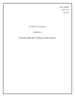
Graph 1: Boxplot 1
By observing Graph 1, there is clear evidence of an outlier in the sample. This outlier is pulling the mean
value away from the center of the data, and stretching the standard deviation. The Quantile-Quantile plot
below will measure the skew of the data.
Graph 2: Q-Q Plot 2
As exemplified in Graph 2, there is quite a significant skew in the sample. This is made apparent by the
plot points deviating significantly from the t-distribution line. Due to the skew and the extreme outlier,
we cannot use a t-distribution to analyze the sample data.
With 98% Lower Confidence Interval for Mean
Distribution of weight
98% Confidence98% Confidence
0
20
40
60
Percent
Kernel
Normal
0
20
40
60
Percent
Kernel
Normal
14.0 14.2 14.4 14.6
weight
-1 0 1
Quantile
14.0
14.2
14.4
weight
Q-Q Plot of weight

6. 6
The following code removes the outlier, and performs the same tests to measure distribution and skew.
/************************************************************************************/
ODS RTF;
Data boxes;
Input weight @@;
Datalines;
14.02 13.97 14.1 14.12 14.10 14.15 14.51 13.97 14.05 14.04 14.11 14.12 14.02
;
Run;
Proc Print data=boxes; /To view all of the data/
Run;
Data nooutlier; /Creates No Outlier dataset/
set boxes;
if weight >=14.27 then delete; /Parameters set by observing the boxplot/
Run;
Proc print data=nooutlier; /To test new dataset/
Run;
Proc TTEST data=nooutlier plots sides=LL h0=14 alpha=.02;
var weight;
Run;
Proc Means data=nooutlier n mean stddev clm alpha=.02 maxdec=10;
var weight;
Title "98% Confidence Interval on Weight of Cereal Boxes";
Run;
ODS RTF CLOSE;
/***********************************************************************************/

7. 7
Graph 4: Boxplot 2
Graph 4 displays a more normal distribution. The mean is more centered in the boxplot, creating an
average that may be more representative of the population mean.
Graph 5: Q-Q plot 2
Graph 5 demonstrates data that is closer to the t-distribution line. There is skew, but it is not significant.
Therefore, we can use a t-test. Below is an analysis of the confidence intervals with and without the
outlier.
With 98% Lower Confidence Interval for Mean
Distribution of weight
98% Confidence98% Confidence
0
10
20
30
40
Percent
Kernel
Normal
0
10
20
30
40
Percent
Kernel
Normal
14.0 14.1 14.2
weight
-1 0 1
Quantile
13.95
14.00
14.05
14.10
14.15
weight
Q-Q Plot of weight

8. 8
STEP 5: Confidence Interval with Outlier
The TTEST Procedure
Variable: Weight
Mean
98% CL
Mean Std Dev
98% CL Std
Dev
14.0642 -Infty 14.1050 0.0608 0.0406 0.1154
MEANS procedure
Confidence Interval (13.998-14.2): Based on how confidence intervals are calculated, we are
98% confident that the mean weight of the cereal boxes is between 13.998oz and 14.20oz. This
conclusion allows us to retain the null hypothesis, as the estimate of 14oz is contained within
the confidence interval.
Margin of Error= .046oz
14.2−13.996
2
=.010 oz
Based on how we calculate confidence intervals, we have concluded that there is a 98% chance
that our estimate mean of 14.064 ounces is the true average plus or minus .046 ounces.
N Mean Std Dev Std Err Minimum Maximum
12 14.0642 0.0608 0.0176 13.9700 14.1500
DF t Value Pr < t
11 3.65 0.9981
Analysis Variable : weight
N Mean Std Dev
Lower 98%
CL for Mean
Upper 98%
CL for Mean
12 14.0641667 0.0608214 14.0164437 14.1118897

9. 9
STEP 6: Confidence Interval without Outlier
The TTEST Procedure
Variable: Weight
Mean
98% CL
Mean Std Dev
98% CL Std
Dev
14.0642 -Infty 14.1050 0.0608 0.0406 0.1154
MEANS Procedure
Confidence Interval (14.01-14.11): Based on how confidence intervals are calculated, we
are 98% confident that the mean weight of the cereal boxes is between 14.01 ounces and
14.11 ounces. This conclusion allows us to reject the null hypothesis, as the estimate of 14
ounces is not contained within the confidence interval.
Margin of Error:
=
14.11−14.01
2
=.05oz
This value means that we are 98% confident that the true mean of the cereal boxes is 14.06
ounces plus or minus .05 ounces.
Conclusion: Upon analyzing the two confidence intervals, it is apparent that the outlier
increases the standard deviation, and stretches out the average of the data. Excluding the
outlier yields an entirely different result as it shows that we are unable to retain our null
hypothesis. For this instance, it may be better to take a larger sample size to get a better
representation of the population as a whole.
N Mean Std Dev Std Err Minimum Maximum
12 14.0642 0.0608 0.0176 13.9700 14.1500
DF t Value Pr < t
11 3.65 0.9981
Analysis Variable : weight
N Mean Std Dev
Lower 98%
CL for Mean
Upper 98%
CL for Mean
12 14.0641667 0.0608214 14.0164437 14.1118897

10. 10
STEP 7: Distribution and Interpretation
t-value: The sample average of 14.06 ounces is 3.65 standard errors to the right of the
hypothesized average of 14 ounces.
p-value: The probability of getting the sample average of 14.06 ounces or lower is
99% when the true average is 14 ounces.
Conclusion: The p-value of .99 is greater than .02 alpha (the significance level necessary
to be 98% confident) so we conclude that the data is not significant. In other
words, since the confidence level does not include the hypothesized
14ounces, we cannot confidently accept the null. Similarly, the data has
shown to not fit the alternative hypothesis either, making it statistically
insignificant.