SlideShare a Scribd company logo
1 of 20
Download to read offline
Harcourt, Inc. items and derived items copyright © 2002 by Harcourt, Inc. Answers and Solutions: 14 - 1
Chapter 14
Cash Flow Estimation and Risk Analysis
ANSWERS TO END-OF-CHAPTER QUESTIONS
14-1 a. Cash flow, which is the relevant financial variable, represents the
actual flow of cash. Accounting income, on the other hand, reports
accounting data as defined by Generally Accepted Accounting Principles
(GAAP).
b. Incremental cash flows are those cash flows that arise solely from the
asset that is being evaluated. For example, assume an existing machine
generates revenues of $1,000 per year and expenses of $600 per year. A
machine being considered as a replacement would generate revenues of
$1,000 per year and expenses of $400 per year. On an incremental
basis, the new machine would not increase revenues at all, but would
decrease expenses by $200 per year. Thus, the annual incremental cash
flow is a before-tax savings of $200. A sunk cost is one that has
already occurred and is not affected by the capital project decision.
Sunk costs are not relevant to capital budgeting decisions. Within the
context of this chapter, an opportunity cost is a cash flow which a
firm must forgo to accept a project. For example, if the project
requires the use of a building which could otherwise be sold, the
market value of the building is an opportunity cost of the project.
c. Net operating working capital changes are the increases in current
operating assets resulting from accepting a project less the resulting
increases in current operting liabilities, or accruals and accounts
payable. A net operating working capital change must be financed just
as a firm must finance its increases in fixed assets.
d. Salvage value is the market value of an asset after its useful life.
Salvage values and their tax effects must be included in project cash
flow estimation.
e. The real rate of return (kr), or, for that matter the real cost of
capital, contains no adjustment for expected inflation. If net cash
flows from a project do not include inflation adjustments, then the
cash flows should be discounted at the real cost of capital. In a
similar manner, the IRR resulting from real net cash flows should be
compared with the real cost of capital. Conversely, the nominal rate
of return (kn) does include an inflation adjustment (premium). Thus if
nominal rates of return are used in the capital budgeting process, the
net cash flows must also be nominal.
f. Sensitivity analysis indicates exactly how much NPV will change in
Answers and Solutions: 14 - 2 Harcourt, Inc. items and derived items copyright © 2002 by Harcourt, Inc.
response to a given change in an input variable, other things held
constant. Sensitivity analysis is sometimes called “what if” analysis
because it answers this type of question.
g. A firm’s worst-case scenario is when all of the variables used in an
analysis are set at their worst reasonably forecasted values. On the
other hand, a best-case scenario sets all input variables at their best
reasonably forecasted values. The worst-and best-case scenarios are
then compared to a base-case in which input values are set at their
most likely values.
h. Scenario analysis is a shorter version of simulation analysis that uses
only a few outcomes. Often the outcomes considered are optimistic,
pessimistic and most likely.
i. Monte Carlo simulation analysis is a risk analysis technique in which a
computer is used to simulate probable future events and thus to
estimate the profitability and risk of a project.
j. The coefficient of variation is a standardized risk measure, obtained
by dividing the standard deviation of a variable by the expected value
of that variable. Since the coefficient of variation is standardized,
it can be used to compare the relative stand-alone risk of projects
which differ in NPV size. The standard deviation measures the
variability of the distribution about the expected value.
k. Corporate diversification involves acquiring assets whose returns are
not highly correlated with the firm’s other assets. The major stated
objectives of corporate diversification are to stabilize earnings and
reduce corporate risk. Stockholder diversification occurs when
stockholders hold a well-diversified portfolio of many companies.
There is some disagreement over the benefits of corporate diversifi-
cation to reduce risk when investors can accomplish the same result
more easily. Under some circumstances, however, diversification
benefits may only arise from corporate diversification.
l. A risk-adjusted discount rate incorporates the riskiness of the
project’s cash flows. The cost of capital to the firm reflects the
average risk of the firm’s existing projects. Thus, new projects that
are riskier than existing projects should have a higher risk-adjusted
discount rate. Conversely, projects with less risk should have a lower
risk-adjusted discount rate. This adjustment process also applies to a
firm’s divisions. Risk differences are difficult to quantify, thus
risk adjustments are often subjective in nature. A project’s cost of
capital is its risk-adjusted discount rate for that project.
14-2 Only cash can be spent or reinvested, and since accounting profits do not
represent cash, they are of less fundamental importance than cash flows
for investment analysis. Recall that in the stock valuation chapters we
focused on dividends and free cash flows, which represent cash flows,
rather than on earnings per share, which represent accounting profits.
Harcourt, Inc. items and derived items copyright © 2002 by Harcourt, Inc. Answers and Solutions: 14 - 3
14-3 Since the cost of capital includes a premium for expected inflation,
failure to adjust cash flows means that the denominator, but not the
numerator, rises with inflation, and this lowers the calculated NPV.
14-4 Capital budgeting analysis should only include those cash flows which will
be affected by the decision. Sunk costs are unrecoverable and cannot be
changed, so they have no bearing on the capital budgeting decision.
Opportunity costs represent the cash flows the firm gives up by investing
in this project rather than its next best alternative, and externalities
are the cash flows (both positive and negative) to other projects that
result from the firm taking on this project. These cash flows occur only
because the firm took on the capital budgeting project; therefore, they
must be included in the analysis.
14-5 When a firm takes on a new capital budgeting project, it typically must
increase its investment in receivables and inventories, over and above the
increase in payables and accruals, thus increasing its net operating
working capital. Since this increase must be financed, it is included as
an outflow in Year 0 of the analysis. At the end of the project’s life,
inventories are depleted and receivables are collected. Thus, there is a
decrease in NOWC, which is treated as an inflow.
14-6 Simulation analysis involves working with continuous probability
distributions, and the output of a simulation analysis is a distribution
of net present values or rates of return. Scenario analysis involves
picking several points on the various probability distributions and
determining cash flows or rates of return for these points. Sensitivity
analysis involves determining the extent to which cash flows change, given
a change in one particular input variable. Simulation analysis is
expensive. Therefore, it would more than likely be employed in the
decision for the $200 million investment in a satellite system than in the
decision for the $12,000 truck.
14-7 Beta (market) risk refers to the project’s effect on the corporate beta
coefficient. Within-firm (corporate) risk refers to the project’s effect
on the stability of the firm’s earnings. Stand-alone risk refers to the
inherent riskiness of the project’s expected returns when viewed alone.
Theoretically, beta (market) risk should be given greater weight for
publicly held firms, but from a practical standpoint, within-firm
(corporate) risk is probably considered more important.
Answers and Solutions: 14 - 4 Harcourt, Inc. items and derived items copyright © 2002 by Harcourt, Inc.
SOLUTIONS TO END-OF-CHAPTER PROBLEMS
14-1 Equipment $ 9,000,000
NWC Investment 3,000,000
Initial investment outlay $12,000,000
14-2 Operating Cash Flows: t = 1
Sales revenues $10,000,000
Operating costs 7,000,000
Depreciation 2,000,000
Operating income before taxes $ 1,000,000
Taxes (40%) 400,000
Operating income after taxes $ 600,000
Add back depreciation 2,000,000
Operating cash flow $ 2,600,000
14-3 Equipment's original cost $20,000,000
Depreciation (80%) 16,000,000
Book value $ 4,000,000
Gain on sale = $5,000,000 - $4,000,000 = $1,000,000.
Tax on gain = $1,000,000(0.4) = $400,000.
AT net salvage value = $5,000,000 - $400,000 = $4,600,000.
14-4 a. The net cost is $126,000:
Price ($108,000)
Modification (12,500)
Increase in NWC (5,500)
Cash outlay for new machine ($126,000)
b. The operating cash flows follow:
Year 1 Year 2 Year 3
1. After-tax savings $28,600 $28,600 $28,600
2. Depreciation tax savings 13,918 18,979 6,326
Net cash flow $42,518 $47,579 $34,926
Notes:
1. The after-tax cost savings is $44,000(1 - T) = $44,000(0.65)
= $28,600.
2. The depreciation expense in each year is the depreciable basis,
$120,500, times the MACRS allowance percentages of 0.33, 0.45, and
Harcourt, Inc. items and derived items copyright © 2002 by Harcourt, Inc. Answers and Solutions: 14 - 5
0.15 for Years 1, 2, and 3, respectively. Depreciation expense in
Years 1, 2, and 3 is $39,765, $54,225, and $18,075. The
depreciation tax savings is calculated as the tax rate (35%) times
the depreciation expense in each year.
c. The terminal year cash flow is $50,702:
Salvage value $65,000
Tax on SV* (19,798)
Return of NWC 5,500
$50,702
BV in Year 4 = $120,500(0.07) = $8,435.
*Tax on SV = ($65,000 - $8,435)(0.35) = $19,798.
d. The project has an NPV of $10,841; thus, it should be accepted.
Year Net Cash Flow PV @ 12%
0 ($126,000) ($126,000)
1 42,518 37,963
2 47,579 37,930
3 85,628 60,948
NPV = $ 10,841
Alternatively, place the cash flows on a time line:
0 1 2 3
| | | |
-126,000 42,518 47,579 34,926
50,702
85,628
With a financial calculator, input the appropriate cash flows into the
cash flow register, input I = 12, and then solve for NPV = $10,841.
14-5 Year MACRS S-L Dep ∆Dep T(∆Dep)
0 0 0 0 0
1 $5,000,000 $5,000,000 0 0
2 9,000,000 5,000,000 $4,000,000 $1,360,000
3 7,000,000 5,000,000 2,000,000 680,000
4 6,000,000 5,000,000 1,000,000 340,000
5 4,500,000 5,000,000 ( 500,000) ( 170,000)
6 3,500,000 5,000,000 (1,500,000) ( 510,000)
7 3,500,000 5,000,000 (1,500,000) ( 510,000)
8 3,500,000 5,000,000 (1,500,000) ( 510,000)
9 3,500,000 5,000,000 (1,500,000) ( 510,000)
10 3,000,000 5,000,000 (2,000,000) ( 680,000)
11 1,500,000 0 1,500,000 510,000
PV @ 10% = $674,311
12%
Answers and Solutions: 14 - 6 Harcourt, Inc. items and derived items copyright © 2002 by Harcourt, Inc.
With a financial calculator, input the following: CF0 = 0, CF1 = 0,
CF2 = 1360000, CF3 = 680000, CF4 = 340000, CF5 = -170000, CF6 = -510000, Nj
= 4, CF10 = -680000, CF11 = 510000, and I = 10 to solve for NPV =
$674,310.51.
Therefore, the value of the firm would increase by $674,311, each year,
if it elected to use standard MACRS depreciation rates.
14-6 a. The net cost is $89,000:
Price ($70,000)
Modification (15,000)
Change in NWC (4,000)
($89,000)
b. The operating cash flows follow:
Year 1 Year 2 Year 3
After-tax savings $15,000 $15,000 $15,000
Depreciation shield 11,220 15,300 5,100
Net cash flow $26,220 $30,300 $20,100
Notes:
1. The after-tax cost savings is $25,000(1 – T) = $25,000(0.6)
= $15,000.
2. The depreciation expense in each year is the depreciable basis,
$85,000, times the MACRS allowance percentage of 0.33, 0.45, and
0.15 for Years 1, 2 and 3, respectively. Depreciation expense in
Years 1, 2, and 3 is $28,050, $38,250, and $12,750. The
depreciation shield is calculated as the tax rate (40%) times the
depreciation expense in each year.
c. The additional end-of-project cash flow is $24,380:
Salvage value $30,000
Tax on SV* (9,620)
Return of NWC 4,000
$24,380
*Tax on SV = ($30,000 - $5,950)(0.4) = $9,620.
Note that the remaining BV in Year 4 = $85,000(0.07) = $5,950.
d. The project has an NPV of -$6,705. Thus, it should not be accepted.
Year Net Cash Flow PV @ 10%
0 ($89,000) ($89,000)
1 26,220 23,836
2 30,300 25,041
3 44,480 33,418
Harcourt, Inc. items and derived items copyright © 2002 by Harcourt, Inc. Answers and Solutions: 14 - 7
NPV = ($ 6,705)
Alternatively, with a financial calculator, input the following: CF0 =
-89000, CF1 = 26220, CF2 = 30300, CF3 = 44480, and I = 10 to solve for
NPV = -$6,703.83.
14-7 a. Sales = 1,000($138) $138,000
Cost = 1,000($105) 105,000
Net before tax $ 33,000
Taxes (34%) 11,220
Net after tax $ 21,780
Not considering inflation, NPV is -$4,800. This value is calculated as
-$150,000 +
15.0
780,21$
= -$4,800.
Considering inflation, the real cost of capital is calculated as
follows:
(1 + kr)(1 + i) = 1.15
(1 + kr)(1.06) = 1.15
kr = 0.0849.
Thus, the NPV considering inflation is calculated as
-$150,000 +
0849.0
780,21$
= $106,537.
After adjusting for expected inflation, we see that the project has a
positive NPV and should be accepted. This demonstrates the bias that
inflation can induce into the capital budgeting process: Inflation is
already reflected in the denominator (the cost of capital), so it must
also be reflected in the numerator.
b. If part of the costs were fixed, and hence did not rise with inflation,
then sales revenues would rise faster than total costs. However, when
the plant wears out and must be replaced, inflation will cause the
replacement cost to jump, necessitating a sharp output price increase
to cover the now higher depreciation charges.
14-8 E(NPV) = 0.05(-$70) + 0.20(-$25) + 0.50($12) + 0.20($20) + 0.05($30)
= -$3.5 + -$5.0 + $6.0 + $4.0 + $1.5
= $3.0 million.
σNPV = [0.05(-$70 - $3)2
+ 0.20(-$25 - $3)2
+ 0.50($12 - $3)2
+ 0.20($20 - $3)2
+ 0.05($30 - $3)2
]
= $23.622 million.
CV =
$3.0
$23.622
= 7.874.
Answers and Solutions: 14 - 8 Harcourt, Inc. items and derived items copyright © 2002 by Harcourt, Inc.
14-9 a. Expected annual cash flows:
Project A: Probable
Probability × Cash Flow = Cash Flow
0.2 $6,000 $1,200
0.6 6,750 4,050
0.2 7,500 1,500
Expected annual cash flow = $6,750
Project B: Probable
Probability × Cash Flow = Cash Flow
0.2 $ 0 $ 0
0.6 6,750 4,050
0.2 18,000 3,600
Expected annual cash flow = $7,650
Coefficient of variation:
CV =
NPVExpected
=
valueExpected
deviationStandard NPVσ
Project A:
σA = $474.34.=(0.2))($750+(0.6))($0+(0.2))(-$750 222
Project B:
σB = (0.2))($10,350+(0.6))(-$900+(0.2))(-$7,650 222
= $5,797.84.
CVA = $474.34/$6,750 = 0.0703.
CVB = $5,797.84/$7,650 = 0.7579.
b. Project B is the riskier project because it has the greater variability
in its probable cash flows, whether measured by the standard deviation
or the coefficient of variation. Hence, Project B is evaluated at the
12 percent cost of capital, while Project A requires only a 10 percent
cost of capital.
Project A: With a financial calculator, input the appropriate cash
flows into the cash flow register, input I = 10, and then solve for
NPV = $10,036.25.
Project B: With a financial calculator, input the appropriate cash
flows into the cash flow register, input I = 12, and then solve for NPV
= $11,624.01.
Project B has the higher NPV; therefore, the firm should accept
Project B.
Harcourt, Inc. items and derived items copyright © 2002 by Harcourt, Inc. Answers and Solutions: 14 - 9
c. The portfolio effects from Project B would tend to make it less risky
than otherwise. This would tend to reinforce the decision to accept
Project B. Again, if Project B were negatively correlated with the GDP
(Project B is profitable when the economy is down), then it is less
risky and Project B’s acceptance is reinforced.
14-10 a. First, note that with symmetric probability distributions, the middle
value of each distribution is the expected value. Therefore,
Expected Values
Sales (units) 200
Sales price $13,500
Sales in dollars $2,700,000
Costs (200 x $6,000) 1,200,000
Earnings before taxes $1,500,000
Taxes (40%) 600,000
Net income $ 900,000 = Cash flow under the
assumption used in the
problem.
0 = ∑= +
8
1t
t
)IRR1(
000,900$
- $4,000,000.
Using a financial calculator, input the following: CF0 = -4000000,
CF1 = 900000, and Nj = 8, to solve for IRR = 15.29%.
Expected IRR = 15.29% 15.3%.
Assuming complete independence between the distributions, and
normality, it would be possible to derive σIRR statistically.
Alternatively, we could employ simulation to develop a distribution of
IRRs, hence σIRR. There is no easy way to get σIRR.
b. NPV = $900,000(PVIFA15%,8) - $4,000,000.
Using a financial calculator, input the following: CF0 = -4000000,
CF1 = 900000, Nj = 8, and I = 15 to solve for NPV = $38,589.36. Again,
there is no easy way to estimate σNPV.
c. (1) a. Calculate developmental costs. The 44 random number value,
coming between 30 and 70, indicates that the costs for this run
should be taken to be $4 million.
b. Calculate the project life. The 17, being less than 20,
indicates that a 3-year life should be used.
(2) a. Estimate unit sales. The 16 indicates sales of 100 units.
Answers and Solutions: 14 - 10 Harcourt, Inc. items and derived items copyright © 2002 by Harcourt, Inc.
b. Estimate the sales price. The 58 indicates a sales price of
$13,500.
c. Estimate the cost per unit. The 1 indicates a cost of $5,000.
d. Now estimate the after-tax cash flow for Year 1. It is
[100($13,500) - 100($5,000)](1 - 0.4) = $510,000 = CF1.
(3) Repeat the process for Year 2. Sales will be 200 with a random
number of 79; the price will be $13,500 with a random number of 83;
and the cost will be $7,000 with a random number of 86:
[200($13,500) - 200($7,000)](0.6) = $780,000 = CF2.
(4) Repeat the process for Year 3. Sales will be 100 units with a
random number of 19; the price will be $13,500 with a random number
of 62; and the cost will be $5,000 with a random number of 6:
[100($13,500) - 100($5,000)](0.6) = $510,000 = CF3.
(5) a. 0 = 321
)IRR1(
000,510$
)IRR1(
000,780$
)IRR1(
000,510$
+
+
+
+
+
- $4,000,000
IRR = -31.55%.
Alternatively, with a financial calculator, input the
following: CF0 = -4000000, CF1 = 510000, CF2 = 780000, CF3 =
510000, and solve for IRR = -31.55%.
b. NPV = 321
)15.1(
000,510$
)15.1(
000,780$
)15.1(
000,510$
++ - $4,000,000.
With a financial calculator, input the following: CF0 =
-4000000, CF1 = 510000, CF2 = 780000, CF3 = 510000, and I = 15
to solve for NPV = -$2,631,396.40.
The results of this run are very bad because the project’s
life is so short. Had the life turned out (by chance) to be
13 years, the longest possible life, the IRR would have been
about 25%, and the NPV would have been about $1 million.
(6) & (7) The computer would store σNPVs and σIRRs for the different
trials, then display them as frequency distributions:
Harcourt, Inc. items and derived items copyright © 2002 by Harcourt, Inc. Answers and Solutions: 14 - 11
Probability
of occurrence
X
XX
XXXX
XXXXXXXX
XXXXXXXXXXXXXXX
XXXXXXXXXXXXXXXXXXX
0 E(NPV) NPV
Probability
of occurrence
X
XX
XXXX
XXXXXXXX
XXXXXXXXXXXXXXX
XXXXXXXXXXXXXXXXXXX
0 E(NPV) NPV
The distribution would be reasonably symmetrical because all
the input data were from symmetrical distributions. One
often finds, however, that the input and output
distributions are badly skewed. The frequency values would
also be used to calculate σNPV and σIRR; these values would be
printed out and available for analysis.
d. It’s not strange--the risk analysis should be used as a basis for
setting the cost of capital for use in the NPV method. What can be
done is to discount at the risk-free rate to get an NPV which simply
reflects the timing of cash flows, then to use the variability of this
NPV distribution to establish the project’s riskiness, and finally to
conduct a second simulation with a risk-adjusted cost of capital before
making the final go/no-go decision on the project.
e. Dependence among the variables listed could either decrease or increase
the dispersion of the NPV distribution, depending on the type of
correlations assumed. For example, if we assume that high unit sales
are associated with strong market prices, and that high volume brings
low unit costs because of scale economies, then the NPV would probably
widen. If we assume intertemporal dependence--for example, that strong
demand in Year 1 signifies good product acceptance, hence strong sales
in Years 2 to n, this will definitely increase NPV and IRR, because
good and bad events will not cancel one another out, but will be
reinforcing. However, if we assume that low prices will produce high
unit sales, then FNPV would probably decrease.
f. The biggest problem is getting good data on probability distributions,
and especially on correlations among the input variables such as among
unit sales, sales prices, and unit costs. The second major problem is
Answers and Solutions: 14 - 12 Harcourt, Inc. items and derived items copyright © 2002 by Harcourt, Inc.
a conceptual one--this type of analysis does not deal at all with
market (or beta) risk. A project with a high FNPV or FIRR may not be
strongly correlated with “the market,” or may even be negatively
correlated, making FNPV and FIRR not very useful as an indicator of risk.
Harcourt, Inc. items and derived items copyright © 2002 by Harcourt, Inc. Solution to Spreadsheet Problems: 14 - 13
SOLUTION TO SPREADSHEET PROBLEMS
14-11 The detailed solution for the problem is available both on the
instructor’s resource CD-ROM (in the file Solution for Ch 14-11 Build a
Model.xls) and on the instructor’s side of the Harcourt College
Publishers’ web site, http://www.harcourtcollege.com/finance/theory10e.
14-12 a. The net cost is $212,500:
Price ($180,000)
Modification (25,000)
Change in NWC (7,500)
($212,500)
b. The operating cash flows follow:
Year 1 Year 2 Year 3
1. After-tax savings $49,500 $49,500 $49,500
2. Depreciation tax savings 23,001 31,365 10,455
Net cash flow $72,501 $80,865 $59,955
Notes:
1. The after-tax cost savings is $75,000(1 - T) = $75,000(0.66)
= $49,500.
2. The depreciation expense in each year is the depreciable basis,
$205,000, times the MACRS allowance percentage of 0.33, 0.45, and
0.15 for Years 1, 2 and 3, respectively. Depreciation expense in
Years 1, 2, and 3 is $67,650, $92,250, and $30,750. The
depreciation shield is calculated as the tax rate (34%) times the
depreciation expense in each year.
c. The end-of-project net cash flow is $65,179:
Salvage value $80,000
Tax on SV* (22,321)
Return of NWC 7,500
$65,179
*Tax on SV = ($80,000 - $14,350)(0.34) = $22,321.
BV in Year 4 = $205,000(0.07) = $14,350.
d. The project has an NPV of $14,256; thus, it should be accepted.
Year Net Cash Flow PV @ 10%
0 ($212,500) ($212,500)
1 72,501 65,910
2 80,865 66,831
3 125,134 94,015
NPV = $ 14,256
Solution to Spreadsheet Problems: 14 - 14 Harcourt, Inc. items and derived items copyright © 2002 by Harcourt, Inc.
Alternatively, using a financial calculator, input the following: CF0 =
-212500, CF1 = 72501, CF2 = 80865, CF3 = 125134, and I = 10 to solve for
NPV = $14,255.60.
e. (1) NPV = $5,766 at k = 12%; (2) NPV = $23,295 at k = 8%.
f. NPV = ($620) and $19,214. If the salvage value were as low as $50,000,
the NPV would be negative; therefore, the uncertainty about the salvage
value could cause the project to be rejected. A salvage value of
$51,251 (rounded to $51,000) would make you indifferent to the project.
g. NPV = $5,256 if the tax rate were changed to 46%.
h. When the base price of the machine is increased to $200,000, the NPV is
($52). You would be indifferent to the project at a machine cost of
$199,928 (rounded to $199,900).
14-13 a. Nominal WACC:
kn = WACC = wdkd(1 - T) + wceks = 0.5(12%)(1 - 0.4) + 0.5(16%)
= 3.6% + 8.0% = 11.6%.
Real WACC:
kr = (kn - i)/(1 + i) = (11.6% - 6%)/(1 + 0.06) = 5.6%/1.06 = 5.28%.
b. The relevant real cash flows are:
0 1 2 3
($18,800) $5,100a
$5,100 $5,100
2,482b
3,384 1,128
($18,800) $7,582 $8,484 $6,228
a
(R - VC - FC)(1 - T) = ($30,000 - $15,000 - $6,500)(0.60) = $5,100.
b
(Dep)(T) = $6,204(0.4) = $2,482.
When calculating the NPV based upon real cash flows, the firm's real
WACC should be utilized. If the nominal WACC were used, the discount
rate would include an inflation premium, while the cash flows would
not. The calculation would bias NPV downward.
c. Using a financial calculator, input the following: CF0 = -18800,
CF1 = 7582, CF2 = 8484, CF3 = 6228, and I = 5.28 to solve for NPV =
$1,393.28 $1,393. Therefore, the project should be accepted. If the
analyst had used the nominal WACC with real cash flows, an erroneous
reject decision would have been made.
NPVat 5.28% = -$18,800 + 1
)0528.1(
582,7$
+ 2
)0528.1(
484,8$
+
)0528.1(
228,6$
= $1,392.
NPVat 11.6% = -$18,800 + 1
)116.1(
582,7$
+ 2
)116.1(
484,8$
+ 3
)116.1(
228,6$
= $-713.7.
Harcourt, Inc. items and derived items copyright © 2002 by Harcourt, Inc. Solution to Spreadsheet Problems: 14 - 15
d. First, we must determine the relevant nominal cash flows:
0 1 2 3
Investment ($18,800)
Rev $31,800 $33,708 $35,730
VC 15,900 16,854 17,865
FC 6,890 7,303 7,742
Net Rev $ 9,010 $ 9,551 $10,123
Net Rev (1 - T) $ 5,406 $ 5,731 $ 6,074
Dep (T) 2,482 3,384 1,128
Net CF $ 7,888 $ 9,115 $ 7,202
Now, since these are nominal cash flows, the NPV can be found using the
nominal WACC:
NPV = -$18,800 + 1
)116.1(
888,7$
+ 2
)116.1(
115,9$
+ 3
)116.1(
202,7$
= $768.
Alternatively, with a financial calculator, input the following: CF0 =
-18800, CF1 = 7888, CF2 = 9115, CF3 = 7202, and I = 11.6 to solve for
NPV = $768.26.
The NPV is less than that found in Part c because the depreciation
savings do not increase with inflation.
e. The relevant after-tax cash flows are:
0 1 2 3
Investment ($18,800)
Rev $31,800 $33,708 $35,730
VC 16,125 17,334 18,634
FC 6,988 7,512 8,075
Net Rev $ 8,687 $ 8,862 $ 9,021
Net Rev (1 - T) $ 5,212 $ 5,317 $ 5,413
Dep (T) 2,482 3,384 1,128
Net CF $ 7,694 $ 8,701 $ 6,541
With a financial calculator, input the following: CF0 = -18800, CF1 =
7694, CF2 = 8701, CF3 = 6541, and I = 11.6 to solve for NPV = -$213.54
-$214.
The unanticipated inflation premium would have caused the project's
NPV to decrease from $768 (as calculated in part d) to -$214. This
would have caused the project to decrease the value of the firm by
$214.
f. (1) Biases would occur--projects' cash flows would not be adjusted for
inflation, but the market cost of capital would be, hence NPVs
would be downward biased.
(2) Long-term projects would have a greater downward bias because of
the compounding in the denominator of the NPV equation.
(3) Cash flows should be adjusted to reflect expected inflation.
Solution to Spreadsheet Problems: 14 - 16 Harcourt, Inc. items and derived items copyright © 2002 by Harcourt, Inc.
14-14 a. If the actual life is 5 years:
Amount Amount Year PV Factor
before tax after tax Event Occurs at 10% PV
Outflows:
Investment in
new equipment $30,000 $30,000 0 1.0 $30,000
Total PV of outflows $30,000
Inflows:
Revenues $10,000 $ 6,000 1-5 3.7908 $22,745
Depreciation 6,000 2,400 1-5 3.7908 9,098
Total PV of inflows $31,843
NPV = PV(Inflows) - PV(Outflows) $ 1,843
Alternatively, using a financial calculator:
Inputs 5 10 8400 0
Output = -31,842.61
NPV = PV(Inflows) – PV(Outflows) = $31,843 - $30,000 = $1,843.
If the actual life is 4 years:
Amount Amount Year PV Factor
before tax after tax Event Occurs at 10% PV
Inflows:
Revenues $10,000 $6,000 1-4 3.1699 $19,019
Depreciation 6,000 2,400 1-4 3.1699 7,608
Tax savings on loss
at end of Year 4 6,000 2,400 4 0.6830 1,639
Total PV of inflows $28,266
NPV = $28,266 - $30,000 = ($1,734).
Alternatively, using a financial calculator, input the following:
CF0 = -30000, CF1 = 8400, Nj = 3, CF4 = 10800, and I = 10 to solve for
NPV = -$1,733.90 -$1,734.
N I FVPMTPV
Harcourt, Inc. items and derived items copyright © 2002 by Harcourt, Inc. Solution to Spreadsheet Problems: 14 - 17
If the actual life is 8 years:
Amount Amount Year PV Factor
before tax after tax Event Occurs at 10% PV
Inflows:
Revenues $10,000 $6,000 1-8 5.3349 $32,009
Depreciation 6,000 2,400 1-5 3.7908 9,098
Total PV of Inflows $41,107
NPV = $41,107 - $30,000 = $11,107.
Alternatively, using a financial calculator, input the following:
CF0 = -30000, CF1 = 8400, Nj = 5, CF4 = 6000, Nj = 3, and I = 10 to solve
for NPV = $11,107.45 $11,107.
If the life is as low as 4 years (an unlikely event), the
investment will not be desirable. But, if the investment life is
longer than 4 years, the investment will be a good one. Therefore, the
decision will depend on the directors’ confidence in the life of the
tractor. Given the low probability of the tractor’s life being only 4
years, it is likely that the directors will decide to purchase the
tractor.
b. 8% cost of capital; NPV = $3,539. 12% cost of capital; NPV = $280.
NPV is still positive at a 12% cost of capital; therefore, the tractor
should be purchased. The project is not very sensitive because when
the cost of capital is increased by 4% NPV is still positive.
c. At $7,000 operating revenue, NPV = ($4,981). At $13,000 operating
revenue, NPV = $8,666.
With a project life of one year, NPV = ($13,636). With a project life
of ten years, NPV = $15,965.
4% cost of capital; NPV = $7,395. 16% cost of capital; NPV = ($2,496).
Solution to Spreadsheet Problems: 14 - 18 Harcourt, Inc. items and derived items copyright © 2002 by Harcourt, Inc.
NPV
NPV
(Thousandsof$)
10
8
5
3
1
(5)
(3)
7
6
9
4
2
0
(6)
(4)
(2)
(1)
7 9
Pre-tax Revenues
(Thousands of $)
11 13
Sensitivity Diagram
Sensitivity Diagram
NPV vs. Project Life
15
10
20
5
0
(15)
(10)
(5)
97531
NPV
(Thousandsof$)
Project Life
(Years)
NPV
NPV
(Thousandsof$)
Sensitivity Diagram
NPV vs. Cost of Capital
7
5
9
3
1
(3)
(2)
(1)
6
4
8
2
0
1412 1610864
Cost of Capital
(%)
NPV
Harcourt, Inc. items and derived items copyright © 2002 by Harcourt, Inc. Solution to Cyberproblem: 14 - 19
CYBERPROBLEM
14-15 The detailed solution for the cyberproblem is available on the
instructor’s side of the Harcourt College Publishers’ web site:
http://www.harcourtcollege.com/finance/theory10e.
Mini Case: 14 - 20 Harcourt, Inc. items and derived items copyright © 2002 by Harcourt, Inc.

More Related Content

What's hot

Investment appraisal methods p2
Investment appraisal methods p2Investment appraisal methods p2
Investment appraisal methods p2Antonio Alcocer
 
Capital budgeting techniques
Capital budgeting techniquesCapital budgeting techniques
Capital budgeting techniquesIan Isabel
 
chap006 Making Capital Investment Decisions
chap006 Making Capital Investment Decisionschap006 Making Capital Investment Decisions
chap006 Making Capital Investment DecisionsKartika Dwi Rachmawati
 
Valuation and capital budgeting for the levered firm
Valuation and capital budgeting for the levered firmValuation and capital budgeting for the levered firm
Valuation and capital budgeting for the levered firmOnline
 
Complex Investment Decisions
Complex Investment DecisionsComplex Investment Decisions
Complex Investment DecisionsPANKAJ PANDEY
 
Capital Budgeting and Leverages
Capital Budgeting and LeveragesCapital Budgeting and Leverages
Capital Budgeting and LeveragesBhooshan Kanani
 
Capital Budgeting - Discounted Cash Flow Analysis - group syndicate 3
Capital Budgeting - Discounted Cash Flow Analysis - group syndicate 3Capital Budgeting - Discounted Cash Flow Analysis - group syndicate 3
Capital Budgeting - Discounted Cash Flow Analysis - group syndicate 3Kiki Fitria Rahadian
 
10. cash flow in capital budgeting
10. cash flow in capital budgeting10. cash flow in capital budgeting
10. cash flow in capital budgetingAfiqEfendy Zaen
 
6 financial evaluation
6 financial evaluation6 financial evaluation
6 financial evaluationharshgakhar
 
FINANCIAL MANAGEMENT BY FINMANCapital budgeting cash flows diorella badel
FINANCIAL MANAGEMENT BY FINMANCapital budgeting cash flows diorella badelFINANCIAL MANAGEMENT BY FINMANCapital budgeting cash flows diorella badel
FINANCIAL MANAGEMENT BY FINMANCapital budgeting cash flows diorella badelMary Rose Habagat
 
Enterprise dcf valuation 2 –stage and 3 stage
Enterprise dcf valuation 2 –stage and 3 stageEnterprise dcf valuation 2 –stage and 3 stage
Enterprise dcf valuation 2 –stage and 3 stageMD Asgar
 
Financial Management Slides Ch 16
Financial Management Slides Ch 16Financial Management Slides Ch 16
Financial Management Slides Ch 16Sayyed Naveed Ali
 
DiscountedCashFlowAnalysis_FMS
DiscountedCashFlowAnalysis_FMSDiscountedCashFlowAnalysis_FMS
DiscountedCashFlowAnalysis_FMSAntoine Parant
 
Cash flow estimation ppt @ bec doms on finance
Cash flow estimation ppt @ bec doms on financeCash flow estimation ppt @ bec doms on finance
Cash flow estimation ppt @ bec doms on financeBabasab Patil
 
PM Unit III - Project Cash Flows
PM   Unit III - Project Cash FlowsPM   Unit III - Project Cash Flows
PM Unit III - Project Cash FlowsGhaith Al Darmaki
 

What's hot (20)

Estimation of Cash Flow
Estimation of Cash FlowEstimation of Cash Flow
Estimation of Cash Flow
 
Investment appraisal methods p2
Investment appraisal methods p2Investment appraisal methods p2
Investment appraisal methods p2
 
Capital budgeting techniques
Capital budgeting techniquesCapital budgeting techniques
Capital budgeting techniques
 
chap006 Making Capital Investment Decisions
chap006 Making Capital Investment Decisionschap006 Making Capital Investment Decisions
chap006 Making Capital Investment Decisions
 
Capital Budgeting
Capital BudgetingCapital Budgeting
Capital Budgeting
 
Valuation and capital budgeting for the levered firm
Valuation and capital budgeting for the levered firmValuation and capital budgeting for the levered firm
Valuation and capital budgeting for the levered firm
 
Complex Investment Decisions
Complex Investment DecisionsComplex Investment Decisions
Complex Investment Decisions
 
Capital Budgeting and Leverages
Capital Budgeting and LeveragesCapital Budgeting and Leverages
Capital Budgeting and Leverages
 
Capital Budgeting - Discounted Cash Flow Analysis - group syndicate 3
Capital Budgeting - Discounted Cash Flow Analysis - group syndicate 3Capital Budgeting - Discounted Cash Flow Analysis - group syndicate 3
Capital Budgeting - Discounted Cash Flow Analysis - group syndicate 3
 
Chapter 5- capital budgeting
Chapter   5- capital budgetingChapter   5- capital budgeting
Chapter 5- capital budgeting
 
4 the basic of capital budgeting
4 the basic of capital budgeting4 the basic of capital budgeting
4 the basic of capital budgeting
 
09eh2ch13
09eh2ch1309eh2ch13
09eh2ch13
 
10. cash flow in capital budgeting
10. cash flow in capital budgeting10. cash flow in capital budgeting
10. cash flow in capital budgeting
 
6 financial evaluation
6 financial evaluation6 financial evaluation
6 financial evaluation
 
FINANCIAL MANAGEMENT BY FINMANCapital budgeting cash flows diorella badel
FINANCIAL MANAGEMENT BY FINMANCapital budgeting cash flows diorella badelFINANCIAL MANAGEMENT BY FINMANCapital budgeting cash flows diorella badel
FINANCIAL MANAGEMENT BY FINMANCapital budgeting cash flows diorella badel
 
Enterprise dcf valuation 2 –stage and 3 stage
Enterprise dcf valuation 2 –stage and 3 stageEnterprise dcf valuation 2 –stage and 3 stage
Enterprise dcf valuation 2 –stage and 3 stage
 
Financial Management Slides Ch 16
Financial Management Slides Ch 16Financial Management Slides Ch 16
Financial Management Slides Ch 16
 
DiscountedCashFlowAnalysis_FMS
DiscountedCashFlowAnalysis_FMSDiscountedCashFlowAnalysis_FMS
DiscountedCashFlowAnalysis_FMS
 
Cash flow estimation ppt @ bec doms on finance
Cash flow estimation ppt @ bec doms on financeCash flow estimation ppt @ bec doms on finance
Cash flow estimation ppt @ bec doms on finance
 
PM Unit III - Project Cash Flows
PM   Unit III - Project Cash FlowsPM   Unit III - Project Cash Flows
PM Unit III - Project Cash Flows
 

Similar to Ch14sol cash flow estimation

PPAM-AK PPT.pptx
PPAM-AK PPT.pptxPPAM-AK PPT.pptx
PPAM-AK PPT.pptxShyam273559
 
Lecture cash flow evaluation new
Lecture cash flow evaluation newLecture cash flow evaluation new
Lecture cash flow evaluation newBsgr Planmin
 
Lecture cash flow evaluation new
Lecture cash flow evaluation newLecture cash flow evaluation new
Lecture cash flow evaluation newBsgr Planmin
 
Brad Simon - Finance Lecture - Project Valuation
Brad Simon - Finance Lecture - Project ValuationBrad Simon - Finance Lecture - Project Valuation
Brad Simon - Finance Lecture - Project Valuationbradhapa
 
Project Valuation Lecture
Project Valuation LectureProject Valuation Lecture
Project Valuation Lecturebradhapa
 
Introduction To Capital Budgeting Techniques.ppt
Introduction To Capital Budgeting Techniques.pptIntroduction To Capital Budgeting Techniques.ppt
Introduction To Capital Budgeting Techniques.pptanshikagoel52
 
Capital budgeting methods lecture notes
Capital budgeting methods lecture notesCapital budgeting methods lecture notes
Capital budgeting methods lecture notesWarui Maina
 
237367257 question-case-study-3
237367257 question-case-study-3237367257 question-case-study-3
237367257 question-case-study-3homeworkping3
 
Chapter 10.The Cost of Capital(WACC)
Chapter 10.The Cost of Capital(WACC)Chapter 10.The Cost of Capital(WACC)
Chapter 10.The Cost of Capital(WACC)ZahraMirzayeva
 
Capital Budgeting
Capital BudgetingCapital Budgeting
Capital Budgetingyashpal01
 
Sheet4Assignment 1 LASA # 2—Capital Budgeting TechniquesSheet1So.docx
Sheet4Assignment 1 LASA # 2—Capital Budgeting TechniquesSheet1So.docxSheet4Assignment 1 LASA # 2—Capital Budgeting TechniquesSheet1So.docx
Sheet4Assignment 1 LASA # 2—Capital Budgeting TechniquesSheet1So.docxlesleyryder69361
 
UNIT-4 Capital Budgeting.pdf
UNIT-4 Capital Budgeting.pdfUNIT-4 Capital Budgeting.pdf
UNIT-4 Capital Budgeting.pdfPralayMondal3
 
Financial Tools for Product Managers
Financial Tools for Product ManagersFinancial Tools for Product Managers
Financial Tools for Product ManagersSVPMA
 

Similar to Ch14sol cash flow estimation (20)

PPAM-AK PPT.pptx
PPAM-AK PPT.pptxPPAM-AK PPT.pptx
PPAM-AK PPT.pptx
 
Ch 10
Ch 10Ch 10
Ch 10
 
Lecture cash flow evaluation new
Lecture cash flow evaluation newLecture cash flow evaluation new
Lecture cash flow evaluation new
 
Lecture cash flow evaluation new
Lecture cash flow evaluation newLecture cash flow evaluation new
Lecture cash flow evaluation new
 
Brad Simon - Finance Lecture - Project Valuation
Brad Simon - Finance Lecture - Project ValuationBrad Simon - Finance Lecture - Project Valuation
Brad Simon - Finance Lecture - Project Valuation
 
Project Valuation Lecture
Project Valuation LectureProject Valuation Lecture
Project Valuation Lecture
 
THE COST OF CAPITAL
THE COST OF CAPITALTHE COST OF CAPITAL
THE COST OF CAPITAL
 
Introduction To Capital Budgeting Techniques.ppt
Introduction To Capital Budgeting Techniques.pptIntroduction To Capital Budgeting Techniques.ppt
Introduction To Capital Budgeting Techniques.ppt
 
Cfd ppt
Cfd pptCfd ppt
Cfd ppt
 
Investment decision
Investment decisionInvestment decision
Investment decision
 
Capital budgeting methods lecture notes
Capital budgeting methods lecture notesCapital budgeting methods lecture notes
Capital budgeting methods lecture notes
 
237367257 question-case-study-3
237367257 question-case-study-3237367257 question-case-study-3
237367257 question-case-study-3
 
Chapter 10.The Cost of Capital(WACC)
Chapter 10.The Cost of Capital(WACC)Chapter 10.The Cost of Capital(WACC)
Chapter 10.The Cost of Capital(WACC)
 
ch 12 cost of capital.pdf
ch 12 cost of capital.pdfch 12 cost of capital.pdf
ch 12 cost of capital.pdf
 
Capital Budgeting
Capital BudgetingCapital Budgeting
Capital Budgeting
 
VBM, KPI Feb 2016
VBM, KPI Feb 2016VBM, KPI Feb 2016
VBM, KPI Feb 2016
 
Sheet4Assignment 1 LASA # 2—Capital Budgeting TechniquesSheet1So.docx
Sheet4Assignment 1 LASA # 2—Capital Budgeting TechniquesSheet1So.docxSheet4Assignment 1 LASA # 2—Capital Budgeting TechniquesSheet1So.docx
Sheet4Assignment 1 LASA # 2—Capital Budgeting TechniquesSheet1So.docx
 
UNIT-4 Capital Budgeting.pdf
UNIT-4 Capital Budgeting.pdfUNIT-4 Capital Budgeting.pdf
UNIT-4 Capital Budgeting.pdf
 
capital_budgeting.ppt
capital_budgeting.pptcapital_budgeting.ppt
capital_budgeting.ppt
 
Financial Tools for Product Managers
Financial Tools for Product ManagersFinancial Tools for Product Managers
Financial Tools for Product Managers
 

Recently uploaded

Crayon Activity Handout For the Crayon A
Crayon Activity Handout For the Crayon ACrayon Activity Handout For the Crayon A
Crayon Activity Handout For the Crayon AUnboundStockton
 
18-04-UA_REPORT_MEDIALITERAСY_INDEX-DM_23-1-final-eng.pdf
18-04-UA_REPORT_MEDIALITERAСY_INDEX-DM_23-1-final-eng.pdf18-04-UA_REPORT_MEDIALITERAСY_INDEX-DM_23-1-final-eng.pdf
18-04-UA_REPORT_MEDIALITERAСY_INDEX-DM_23-1-final-eng.pdfssuser54595a
 
EPANDING THE CONTENT OF AN OUTLINE using notes.pptx
EPANDING THE CONTENT OF AN OUTLINE using notes.pptxEPANDING THE CONTENT OF AN OUTLINE using notes.pptx
EPANDING THE CONTENT OF AN OUTLINE using notes.pptxRaymartEstabillo3
 
How to Configure Email Server in Odoo 17
How to Configure Email Server in Odoo 17How to Configure Email Server in Odoo 17
How to Configure Email Server in Odoo 17Celine George
 
Organic Name Reactions for the students and aspirants of Chemistry12th.pptx
Organic Name Reactions  for the students and aspirants of Chemistry12th.pptxOrganic Name Reactions  for the students and aspirants of Chemistry12th.pptx
Organic Name Reactions for the students and aspirants of Chemistry12th.pptxVS Mahajan Coaching Centre
 
call girls in Kamla Market (DELHI) 🔝 >༒9953330565🔝 genuine Escort Service 🔝✔️✔️
call girls in Kamla Market (DELHI) 🔝 >༒9953330565🔝 genuine Escort Service 🔝✔️✔️call girls in Kamla Market (DELHI) 🔝 >༒9953330565🔝 genuine Escort Service 🔝✔️✔️
call girls in Kamla Market (DELHI) 🔝 >༒9953330565🔝 genuine Escort Service 🔝✔️✔️9953056974 Low Rate Call Girls In Saket, Delhi NCR
 
ECONOMIC CONTEXT - LONG FORM TV DRAMA - PPT
ECONOMIC CONTEXT - LONG FORM TV DRAMA - PPTECONOMIC CONTEXT - LONG FORM TV DRAMA - PPT
ECONOMIC CONTEXT - LONG FORM TV DRAMA - PPTiammrhaywood
 
KSHARA STURA .pptx---KSHARA KARMA THERAPY (CAUSTIC THERAPY)————IMP.OF KSHARA ...
KSHARA STURA .pptx---KSHARA KARMA THERAPY (CAUSTIC THERAPY)————IMP.OF KSHARA ...KSHARA STURA .pptx---KSHARA KARMA THERAPY (CAUSTIC THERAPY)————IMP.OF KSHARA ...
KSHARA STURA .pptx---KSHARA KARMA THERAPY (CAUSTIC THERAPY)————IMP.OF KSHARA ...M56BOOKSTORE PRODUCT/SERVICE
 
Employee wellbeing at the workplace.pptx
Employee wellbeing at the workplace.pptxEmployee wellbeing at the workplace.pptx
Employee wellbeing at the workplace.pptxNirmalaLoungPoorunde1
 
Introduction to ArtificiaI Intelligence in Higher Education
Introduction to ArtificiaI Intelligence in Higher EducationIntroduction to ArtificiaI Intelligence in Higher Education
Introduction to ArtificiaI Intelligence in Higher Educationpboyjonauth
 
Painted Grey Ware.pptx, PGW Culture of India
Painted Grey Ware.pptx, PGW Culture of IndiaPainted Grey Ware.pptx, PGW Culture of India
Painted Grey Ware.pptx, PGW Culture of IndiaVirag Sontakke
 
Roles & Responsibilities in Pharmacovigilance
Roles & Responsibilities in PharmacovigilanceRoles & Responsibilities in Pharmacovigilance
Roles & Responsibilities in PharmacovigilanceSamikshaHamane
 
Framing an Appropriate Research Question 6b9b26d93da94caf993c038d9efcdedb.pdf
Framing an Appropriate Research Question 6b9b26d93da94caf993c038d9efcdedb.pdfFraming an Appropriate Research Question 6b9b26d93da94caf993c038d9efcdedb.pdf
Framing an Appropriate Research Question 6b9b26d93da94caf993c038d9efcdedb.pdfUjwalaBharambe
 
Interactive Powerpoint_How to Master effective communication
Interactive Powerpoint_How to Master effective communicationInteractive Powerpoint_How to Master effective communication
Interactive Powerpoint_How to Master effective communicationnomboosow
 
भारत-रोम व्यापार.pptx, Indo-Roman Trade,
भारत-रोम व्यापार.pptx, Indo-Roman Trade,भारत-रोम व्यापार.pptx, Indo-Roman Trade,
भारत-रोम व्यापार.pptx, Indo-Roman Trade,Virag Sontakke
 
Capitol Tech U Doctoral Presentation - April 2024.pptx
Capitol Tech U Doctoral Presentation - April 2024.pptxCapitol Tech U Doctoral Presentation - April 2024.pptx
Capitol Tech U Doctoral Presentation - April 2024.pptxCapitolTechU
 

Recently uploaded (20)

Crayon Activity Handout For the Crayon A
Crayon Activity Handout For the Crayon ACrayon Activity Handout For the Crayon A
Crayon Activity Handout For the Crayon A
 
18-04-UA_REPORT_MEDIALITERAСY_INDEX-DM_23-1-final-eng.pdf
18-04-UA_REPORT_MEDIALITERAСY_INDEX-DM_23-1-final-eng.pdf18-04-UA_REPORT_MEDIALITERAСY_INDEX-DM_23-1-final-eng.pdf
18-04-UA_REPORT_MEDIALITERAСY_INDEX-DM_23-1-final-eng.pdf
 
TataKelola dan KamSiber Kecerdasan Buatan v022.pdf
TataKelola dan KamSiber Kecerdasan Buatan v022.pdfTataKelola dan KamSiber Kecerdasan Buatan v022.pdf
TataKelola dan KamSiber Kecerdasan Buatan v022.pdf
 
EPANDING THE CONTENT OF AN OUTLINE using notes.pptx
EPANDING THE CONTENT OF AN OUTLINE using notes.pptxEPANDING THE CONTENT OF AN OUTLINE using notes.pptx
EPANDING THE CONTENT OF AN OUTLINE using notes.pptx
 
How to Configure Email Server in Odoo 17
How to Configure Email Server in Odoo 17How to Configure Email Server in Odoo 17
How to Configure Email Server in Odoo 17
 
Organic Name Reactions for the students and aspirants of Chemistry12th.pptx
Organic Name Reactions  for the students and aspirants of Chemistry12th.pptxOrganic Name Reactions  for the students and aspirants of Chemistry12th.pptx
Organic Name Reactions for the students and aspirants of Chemistry12th.pptx
 
call girls in Kamla Market (DELHI) 🔝 >༒9953330565🔝 genuine Escort Service 🔝✔️✔️
call girls in Kamla Market (DELHI) 🔝 >༒9953330565🔝 genuine Escort Service 🔝✔️✔️call girls in Kamla Market (DELHI) 🔝 >༒9953330565🔝 genuine Escort Service 🔝✔️✔️
call girls in Kamla Market (DELHI) 🔝 >༒9953330565🔝 genuine Escort Service 🔝✔️✔️
 
Model Call Girl in Bikash Puri Delhi reach out to us at 🔝9953056974🔝
Model Call Girl in Bikash Puri  Delhi reach out to us at 🔝9953056974🔝Model Call Girl in Bikash Puri  Delhi reach out to us at 🔝9953056974🔝
Model Call Girl in Bikash Puri Delhi reach out to us at 🔝9953056974🔝
 
ECONOMIC CONTEXT - LONG FORM TV DRAMA - PPT
ECONOMIC CONTEXT - LONG FORM TV DRAMA - PPTECONOMIC CONTEXT - LONG FORM TV DRAMA - PPT
ECONOMIC CONTEXT - LONG FORM TV DRAMA - PPT
 
KSHARA STURA .pptx---KSHARA KARMA THERAPY (CAUSTIC THERAPY)————IMP.OF KSHARA ...
KSHARA STURA .pptx---KSHARA KARMA THERAPY (CAUSTIC THERAPY)————IMP.OF KSHARA ...KSHARA STURA .pptx---KSHARA KARMA THERAPY (CAUSTIC THERAPY)————IMP.OF KSHARA ...
KSHARA STURA .pptx---KSHARA KARMA THERAPY (CAUSTIC THERAPY)————IMP.OF KSHARA ...
 
Model Call Girl in Tilak Nagar Delhi reach out to us at 🔝9953056974🔝
Model Call Girl in Tilak Nagar Delhi reach out to us at 🔝9953056974🔝Model Call Girl in Tilak Nagar Delhi reach out to us at 🔝9953056974🔝
Model Call Girl in Tilak Nagar Delhi reach out to us at 🔝9953056974🔝
 
Employee wellbeing at the workplace.pptx
Employee wellbeing at the workplace.pptxEmployee wellbeing at the workplace.pptx
Employee wellbeing at the workplace.pptx
 
Introduction to ArtificiaI Intelligence in Higher Education
Introduction to ArtificiaI Intelligence in Higher EducationIntroduction to ArtificiaI Intelligence in Higher Education
Introduction to ArtificiaI Intelligence in Higher Education
 
Painted Grey Ware.pptx, PGW Culture of India
Painted Grey Ware.pptx, PGW Culture of IndiaPainted Grey Ware.pptx, PGW Culture of India
Painted Grey Ware.pptx, PGW Culture of India
 
Roles & Responsibilities in Pharmacovigilance
Roles & Responsibilities in PharmacovigilanceRoles & Responsibilities in Pharmacovigilance
Roles & Responsibilities in Pharmacovigilance
 
Framing an Appropriate Research Question 6b9b26d93da94caf993c038d9efcdedb.pdf
Framing an Appropriate Research Question 6b9b26d93da94caf993c038d9efcdedb.pdfFraming an Appropriate Research Question 6b9b26d93da94caf993c038d9efcdedb.pdf
Framing an Appropriate Research Question 6b9b26d93da94caf993c038d9efcdedb.pdf
 
Interactive Powerpoint_How to Master effective communication
Interactive Powerpoint_How to Master effective communicationInteractive Powerpoint_How to Master effective communication
Interactive Powerpoint_How to Master effective communication
 
भारत-रोम व्यापार.pptx, Indo-Roman Trade,
भारत-रोम व्यापार.pptx, Indo-Roman Trade,भारत-रोम व्यापार.pptx, Indo-Roman Trade,
भारत-रोम व्यापार.pptx, Indo-Roman Trade,
 
ESSENTIAL of (CS/IT/IS) class 06 (database)
ESSENTIAL of (CS/IT/IS) class 06 (database)ESSENTIAL of (CS/IT/IS) class 06 (database)
ESSENTIAL of (CS/IT/IS) class 06 (database)
 
Capitol Tech U Doctoral Presentation - April 2024.pptx
Capitol Tech U Doctoral Presentation - April 2024.pptxCapitol Tech U Doctoral Presentation - April 2024.pptx
Capitol Tech U Doctoral Presentation - April 2024.pptx
 

Ch14sol cash flow estimation

  • 1. Harcourt, Inc. items and derived items copyright © 2002 by Harcourt, Inc. Answers and Solutions: 14 - 1 Chapter 14 Cash Flow Estimation and Risk Analysis ANSWERS TO END-OF-CHAPTER QUESTIONS 14-1 a. Cash flow, which is the relevant financial variable, represents the actual flow of cash. Accounting income, on the other hand, reports accounting data as defined by Generally Accepted Accounting Principles (GAAP). b. Incremental cash flows are those cash flows that arise solely from the asset that is being evaluated. For example, assume an existing machine generates revenues of $1,000 per year and expenses of $600 per year. A machine being considered as a replacement would generate revenues of $1,000 per year and expenses of $400 per year. On an incremental basis, the new machine would not increase revenues at all, but would decrease expenses by $200 per year. Thus, the annual incremental cash flow is a before-tax savings of $200. A sunk cost is one that has already occurred and is not affected by the capital project decision. Sunk costs are not relevant to capital budgeting decisions. Within the context of this chapter, an opportunity cost is a cash flow which a firm must forgo to accept a project. For example, if the project requires the use of a building which could otherwise be sold, the market value of the building is an opportunity cost of the project. c. Net operating working capital changes are the increases in current operating assets resulting from accepting a project less the resulting increases in current operting liabilities, or accruals and accounts payable. A net operating working capital change must be financed just as a firm must finance its increases in fixed assets. d. Salvage value is the market value of an asset after its useful life. Salvage values and their tax effects must be included in project cash flow estimation. e. The real rate of return (kr), or, for that matter the real cost of capital, contains no adjustment for expected inflation. If net cash flows from a project do not include inflation adjustments, then the cash flows should be discounted at the real cost of capital. In a similar manner, the IRR resulting from real net cash flows should be compared with the real cost of capital. Conversely, the nominal rate of return (kn) does include an inflation adjustment (premium). Thus if nominal rates of return are used in the capital budgeting process, the net cash flows must also be nominal. f. Sensitivity analysis indicates exactly how much NPV will change in
  • 2. Answers and Solutions: 14 - 2 Harcourt, Inc. items and derived items copyright © 2002 by Harcourt, Inc. response to a given change in an input variable, other things held constant. Sensitivity analysis is sometimes called “what if” analysis because it answers this type of question. g. A firm’s worst-case scenario is when all of the variables used in an analysis are set at their worst reasonably forecasted values. On the other hand, a best-case scenario sets all input variables at their best reasonably forecasted values. The worst-and best-case scenarios are then compared to a base-case in which input values are set at their most likely values. h. Scenario analysis is a shorter version of simulation analysis that uses only a few outcomes. Often the outcomes considered are optimistic, pessimistic and most likely. i. Monte Carlo simulation analysis is a risk analysis technique in which a computer is used to simulate probable future events and thus to estimate the profitability and risk of a project. j. The coefficient of variation is a standardized risk measure, obtained by dividing the standard deviation of a variable by the expected value of that variable. Since the coefficient of variation is standardized, it can be used to compare the relative stand-alone risk of projects which differ in NPV size. The standard deviation measures the variability of the distribution about the expected value. k. Corporate diversification involves acquiring assets whose returns are not highly correlated with the firm’s other assets. The major stated objectives of corporate diversification are to stabilize earnings and reduce corporate risk. Stockholder diversification occurs when stockholders hold a well-diversified portfolio of many companies. There is some disagreement over the benefits of corporate diversifi- cation to reduce risk when investors can accomplish the same result more easily. Under some circumstances, however, diversification benefits may only arise from corporate diversification. l. A risk-adjusted discount rate incorporates the riskiness of the project’s cash flows. The cost of capital to the firm reflects the average risk of the firm’s existing projects. Thus, new projects that are riskier than existing projects should have a higher risk-adjusted discount rate. Conversely, projects with less risk should have a lower risk-adjusted discount rate. This adjustment process also applies to a firm’s divisions. Risk differences are difficult to quantify, thus risk adjustments are often subjective in nature. A project’s cost of capital is its risk-adjusted discount rate for that project. 14-2 Only cash can be spent or reinvested, and since accounting profits do not represent cash, they are of less fundamental importance than cash flows for investment analysis. Recall that in the stock valuation chapters we focused on dividends and free cash flows, which represent cash flows, rather than on earnings per share, which represent accounting profits.
  • 3. Harcourt, Inc. items and derived items copyright © 2002 by Harcourt, Inc. Answers and Solutions: 14 - 3 14-3 Since the cost of capital includes a premium for expected inflation, failure to adjust cash flows means that the denominator, but not the numerator, rises with inflation, and this lowers the calculated NPV. 14-4 Capital budgeting analysis should only include those cash flows which will be affected by the decision. Sunk costs are unrecoverable and cannot be changed, so they have no bearing on the capital budgeting decision. Opportunity costs represent the cash flows the firm gives up by investing in this project rather than its next best alternative, and externalities are the cash flows (both positive and negative) to other projects that result from the firm taking on this project. These cash flows occur only because the firm took on the capital budgeting project; therefore, they must be included in the analysis. 14-5 When a firm takes on a new capital budgeting project, it typically must increase its investment in receivables and inventories, over and above the increase in payables and accruals, thus increasing its net operating working capital. Since this increase must be financed, it is included as an outflow in Year 0 of the analysis. At the end of the project’s life, inventories are depleted and receivables are collected. Thus, there is a decrease in NOWC, which is treated as an inflow. 14-6 Simulation analysis involves working with continuous probability distributions, and the output of a simulation analysis is a distribution of net present values or rates of return. Scenario analysis involves picking several points on the various probability distributions and determining cash flows or rates of return for these points. Sensitivity analysis involves determining the extent to which cash flows change, given a change in one particular input variable. Simulation analysis is expensive. Therefore, it would more than likely be employed in the decision for the $200 million investment in a satellite system than in the decision for the $12,000 truck. 14-7 Beta (market) risk refers to the project’s effect on the corporate beta coefficient. Within-firm (corporate) risk refers to the project’s effect on the stability of the firm’s earnings. Stand-alone risk refers to the inherent riskiness of the project’s expected returns when viewed alone. Theoretically, beta (market) risk should be given greater weight for publicly held firms, but from a practical standpoint, within-firm (corporate) risk is probably considered more important.
  • 4. Answers and Solutions: 14 - 4 Harcourt, Inc. items and derived items copyright © 2002 by Harcourt, Inc. SOLUTIONS TO END-OF-CHAPTER PROBLEMS 14-1 Equipment $ 9,000,000 NWC Investment 3,000,000 Initial investment outlay $12,000,000 14-2 Operating Cash Flows: t = 1 Sales revenues $10,000,000 Operating costs 7,000,000 Depreciation 2,000,000 Operating income before taxes $ 1,000,000 Taxes (40%) 400,000 Operating income after taxes $ 600,000 Add back depreciation 2,000,000 Operating cash flow $ 2,600,000 14-3 Equipment's original cost $20,000,000 Depreciation (80%) 16,000,000 Book value $ 4,000,000 Gain on sale = $5,000,000 - $4,000,000 = $1,000,000. Tax on gain = $1,000,000(0.4) = $400,000. AT net salvage value = $5,000,000 - $400,000 = $4,600,000. 14-4 a. The net cost is $126,000: Price ($108,000) Modification (12,500) Increase in NWC (5,500) Cash outlay for new machine ($126,000) b. The operating cash flows follow: Year 1 Year 2 Year 3 1. After-tax savings $28,600 $28,600 $28,600 2. Depreciation tax savings 13,918 18,979 6,326 Net cash flow $42,518 $47,579 $34,926 Notes: 1. The after-tax cost savings is $44,000(1 - T) = $44,000(0.65) = $28,600. 2. The depreciation expense in each year is the depreciable basis, $120,500, times the MACRS allowance percentages of 0.33, 0.45, and
  • 5. Harcourt, Inc. items and derived items copyright © 2002 by Harcourt, Inc. Answers and Solutions: 14 - 5 0.15 for Years 1, 2, and 3, respectively. Depreciation expense in Years 1, 2, and 3 is $39,765, $54,225, and $18,075. The depreciation tax savings is calculated as the tax rate (35%) times the depreciation expense in each year. c. The terminal year cash flow is $50,702: Salvage value $65,000 Tax on SV* (19,798) Return of NWC 5,500 $50,702 BV in Year 4 = $120,500(0.07) = $8,435. *Tax on SV = ($65,000 - $8,435)(0.35) = $19,798. d. The project has an NPV of $10,841; thus, it should be accepted. Year Net Cash Flow PV @ 12% 0 ($126,000) ($126,000) 1 42,518 37,963 2 47,579 37,930 3 85,628 60,948 NPV = $ 10,841 Alternatively, place the cash flows on a time line: 0 1 2 3 | | | | -126,000 42,518 47,579 34,926 50,702 85,628 With a financial calculator, input the appropriate cash flows into the cash flow register, input I = 12, and then solve for NPV = $10,841. 14-5 Year MACRS S-L Dep ∆Dep T(∆Dep) 0 0 0 0 0 1 $5,000,000 $5,000,000 0 0 2 9,000,000 5,000,000 $4,000,000 $1,360,000 3 7,000,000 5,000,000 2,000,000 680,000 4 6,000,000 5,000,000 1,000,000 340,000 5 4,500,000 5,000,000 ( 500,000) ( 170,000) 6 3,500,000 5,000,000 (1,500,000) ( 510,000) 7 3,500,000 5,000,000 (1,500,000) ( 510,000) 8 3,500,000 5,000,000 (1,500,000) ( 510,000) 9 3,500,000 5,000,000 (1,500,000) ( 510,000) 10 3,000,000 5,000,000 (2,000,000) ( 680,000) 11 1,500,000 0 1,500,000 510,000 PV @ 10% = $674,311 12%
  • 6. Answers and Solutions: 14 - 6 Harcourt, Inc. items and derived items copyright © 2002 by Harcourt, Inc. With a financial calculator, input the following: CF0 = 0, CF1 = 0, CF2 = 1360000, CF3 = 680000, CF4 = 340000, CF5 = -170000, CF6 = -510000, Nj = 4, CF10 = -680000, CF11 = 510000, and I = 10 to solve for NPV = $674,310.51. Therefore, the value of the firm would increase by $674,311, each year, if it elected to use standard MACRS depreciation rates. 14-6 a. The net cost is $89,000: Price ($70,000) Modification (15,000) Change in NWC (4,000) ($89,000) b. The operating cash flows follow: Year 1 Year 2 Year 3 After-tax savings $15,000 $15,000 $15,000 Depreciation shield 11,220 15,300 5,100 Net cash flow $26,220 $30,300 $20,100 Notes: 1. The after-tax cost savings is $25,000(1 – T) = $25,000(0.6) = $15,000. 2. The depreciation expense in each year is the depreciable basis, $85,000, times the MACRS allowance percentage of 0.33, 0.45, and 0.15 for Years 1, 2 and 3, respectively. Depreciation expense in Years 1, 2, and 3 is $28,050, $38,250, and $12,750. The depreciation shield is calculated as the tax rate (40%) times the depreciation expense in each year. c. The additional end-of-project cash flow is $24,380: Salvage value $30,000 Tax on SV* (9,620) Return of NWC 4,000 $24,380 *Tax on SV = ($30,000 - $5,950)(0.4) = $9,620. Note that the remaining BV in Year 4 = $85,000(0.07) = $5,950. d. The project has an NPV of -$6,705. Thus, it should not be accepted. Year Net Cash Flow PV @ 10% 0 ($89,000) ($89,000) 1 26,220 23,836 2 30,300 25,041 3 44,480 33,418
  • 7. Harcourt, Inc. items and derived items copyright © 2002 by Harcourt, Inc. Answers and Solutions: 14 - 7 NPV = ($ 6,705) Alternatively, with a financial calculator, input the following: CF0 = -89000, CF1 = 26220, CF2 = 30300, CF3 = 44480, and I = 10 to solve for NPV = -$6,703.83. 14-7 a. Sales = 1,000($138) $138,000 Cost = 1,000($105) 105,000 Net before tax $ 33,000 Taxes (34%) 11,220 Net after tax $ 21,780 Not considering inflation, NPV is -$4,800. This value is calculated as -$150,000 + 15.0 780,21$ = -$4,800. Considering inflation, the real cost of capital is calculated as follows: (1 + kr)(1 + i) = 1.15 (1 + kr)(1.06) = 1.15 kr = 0.0849. Thus, the NPV considering inflation is calculated as -$150,000 + 0849.0 780,21$ = $106,537. After adjusting for expected inflation, we see that the project has a positive NPV and should be accepted. This demonstrates the bias that inflation can induce into the capital budgeting process: Inflation is already reflected in the denominator (the cost of capital), so it must also be reflected in the numerator. b. If part of the costs were fixed, and hence did not rise with inflation, then sales revenues would rise faster than total costs. However, when the plant wears out and must be replaced, inflation will cause the replacement cost to jump, necessitating a sharp output price increase to cover the now higher depreciation charges. 14-8 E(NPV) = 0.05(-$70) + 0.20(-$25) + 0.50($12) + 0.20($20) + 0.05($30) = -$3.5 + -$5.0 + $6.0 + $4.0 + $1.5 = $3.0 million. σNPV = [0.05(-$70 - $3)2 + 0.20(-$25 - $3)2 + 0.50($12 - $3)2 + 0.20($20 - $3)2 + 0.05($30 - $3)2 ] = $23.622 million. CV = $3.0 $23.622 = 7.874.
  • 8. Answers and Solutions: 14 - 8 Harcourt, Inc. items and derived items copyright © 2002 by Harcourt, Inc. 14-9 a. Expected annual cash flows: Project A: Probable Probability × Cash Flow = Cash Flow 0.2 $6,000 $1,200 0.6 6,750 4,050 0.2 7,500 1,500 Expected annual cash flow = $6,750 Project B: Probable Probability × Cash Flow = Cash Flow 0.2 $ 0 $ 0 0.6 6,750 4,050 0.2 18,000 3,600 Expected annual cash flow = $7,650 Coefficient of variation: CV = NPVExpected = valueExpected deviationStandard NPVσ Project A: σA = $474.34.=(0.2))($750+(0.6))($0+(0.2))(-$750 222 Project B: σB = (0.2))($10,350+(0.6))(-$900+(0.2))(-$7,650 222 = $5,797.84. CVA = $474.34/$6,750 = 0.0703. CVB = $5,797.84/$7,650 = 0.7579. b. Project B is the riskier project because it has the greater variability in its probable cash flows, whether measured by the standard deviation or the coefficient of variation. Hence, Project B is evaluated at the 12 percent cost of capital, while Project A requires only a 10 percent cost of capital. Project A: With a financial calculator, input the appropriate cash flows into the cash flow register, input I = 10, and then solve for NPV = $10,036.25. Project B: With a financial calculator, input the appropriate cash flows into the cash flow register, input I = 12, and then solve for NPV = $11,624.01. Project B has the higher NPV; therefore, the firm should accept Project B.
  • 9. Harcourt, Inc. items and derived items copyright © 2002 by Harcourt, Inc. Answers and Solutions: 14 - 9 c. The portfolio effects from Project B would tend to make it less risky than otherwise. This would tend to reinforce the decision to accept Project B. Again, if Project B were negatively correlated with the GDP (Project B is profitable when the economy is down), then it is less risky and Project B’s acceptance is reinforced. 14-10 a. First, note that with symmetric probability distributions, the middle value of each distribution is the expected value. Therefore, Expected Values Sales (units) 200 Sales price $13,500 Sales in dollars $2,700,000 Costs (200 x $6,000) 1,200,000 Earnings before taxes $1,500,000 Taxes (40%) 600,000 Net income $ 900,000 = Cash flow under the assumption used in the problem. 0 = ∑= + 8 1t t )IRR1( 000,900$ - $4,000,000. Using a financial calculator, input the following: CF0 = -4000000, CF1 = 900000, and Nj = 8, to solve for IRR = 15.29%. Expected IRR = 15.29% 15.3%. Assuming complete independence between the distributions, and normality, it would be possible to derive σIRR statistically. Alternatively, we could employ simulation to develop a distribution of IRRs, hence σIRR. There is no easy way to get σIRR. b. NPV = $900,000(PVIFA15%,8) - $4,000,000. Using a financial calculator, input the following: CF0 = -4000000, CF1 = 900000, Nj = 8, and I = 15 to solve for NPV = $38,589.36. Again, there is no easy way to estimate σNPV. c. (1) a. Calculate developmental costs. The 44 random number value, coming between 30 and 70, indicates that the costs for this run should be taken to be $4 million. b. Calculate the project life. The 17, being less than 20, indicates that a 3-year life should be used. (2) a. Estimate unit sales. The 16 indicates sales of 100 units.
  • 10. Answers and Solutions: 14 - 10 Harcourt, Inc. items and derived items copyright © 2002 by Harcourt, Inc. b. Estimate the sales price. The 58 indicates a sales price of $13,500. c. Estimate the cost per unit. The 1 indicates a cost of $5,000. d. Now estimate the after-tax cash flow for Year 1. It is [100($13,500) - 100($5,000)](1 - 0.4) = $510,000 = CF1. (3) Repeat the process for Year 2. Sales will be 200 with a random number of 79; the price will be $13,500 with a random number of 83; and the cost will be $7,000 with a random number of 86: [200($13,500) - 200($7,000)](0.6) = $780,000 = CF2. (4) Repeat the process for Year 3. Sales will be 100 units with a random number of 19; the price will be $13,500 with a random number of 62; and the cost will be $5,000 with a random number of 6: [100($13,500) - 100($5,000)](0.6) = $510,000 = CF3. (5) a. 0 = 321 )IRR1( 000,510$ )IRR1( 000,780$ )IRR1( 000,510$ + + + + + - $4,000,000 IRR = -31.55%. Alternatively, with a financial calculator, input the following: CF0 = -4000000, CF1 = 510000, CF2 = 780000, CF3 = 510000, and solve for IRR = -31.55%. b. NPV = 321 )15.1( 000,510$ )15.1( 000,780$ )15.1( 000,510$ ++ - $4,000,000. With a financial calculator, input the following: CF0 = -4000000, CF1 = 510000, CF2 = 780000, CF3 = 510000, and I = 15 to solve for NPV = -$2,631,396.40. The results of this run are very bad because the project’s life is so short. Had the life turned out (by chance) to be 13 years, the longest possible life, the IRR would have been about 25%, and the NPV would have been about $1 million. (6) & (7) The computer would store σNPVs and σIRRs for the different trials, then display them as frequency distributions:
  • 11. Harcourt, Inc. items and derived items copyright © 2002 by Harcourt, Inc. Answers and Solutions: 14 - 11 Probability of occurrence X XX XXXX XXXXXXXX XXXXXXXXXXXXXXX XXXXXXXXXXXXXXXXXXX 0 E(NPV) NPV Probability of occurrence X XX XXXX XXXXXXXX XXXXXXXXXXXXXXX XXXXXXXXXXXXXXXXXXX 0 E(NPV) NPV The distribution would be reasonably symmetrical because all the input data were from symmetrical distributions. One often finds, however, that the input and output distributions are badly skewed. The frequency values would also be used to calculate σNPV and σIRR; these values would be printed out and available for analysis. d. It’s not strange--the risk analysis should be used as a basis for setting the cost of capital for use in the NPV method. What can be done is to discount at the risk-free rate to get an NPV which simply reflects the timing of cash flows, then to use the variability of this NPV distribution to establish the project’s riskiness, and finally to conduct a second simulation with a risk-adjusted cost of capital before making the final go/no-go decision on the project. e. Dependence among the variables listed could either decrease or increase the dispersion of the NPV distribution, depending on the type of correlations assumed. For example, if we assume that high unit sales are associated with strong market prices, and that high volume brings low unit costs because of scale economies, then the NPV would probably widen. If we assume intertemporal dependence--for example, that strong demand in Year 1 signifies good product acceptance, hence strong sales in Years 2 to n, this will definitely increase NPV and IRR, because good and bad events will not cancel one another out, but will be reinforcing. However, if we assume that low prices will produce high unit sales, then FNPV would probably decrease. f. The biggest problem is getting good data on probability distributions, and especially on correlations among the input variables such as among unit sales, sales prices, and unit costs. The second major problem is
  • 12. Answers and Solutions: 14 - 12 Harcourt, Inc. items and derived items copyright © 2002 by Harcourt, Inc. a conceptual one--this type of analysis does not deal at all with market (or beta) risk. A project with a high FNPV or FIRR may not be strongly correlated with “the market,” or may even be negatively correlated, making FNPV and FIRR not very useful as an indicator of risk.
  • 13. Harcourt, Inc. items and derived items copyright © 2002 by Harcourt, Inc. Solution to Spreadsheet Problems: 14 - 13 SOLUTION TO SPREADSHEET PROBLEMS 14-11 The detailed solution for the problem is available both on the instructor’s resource CD-ROM (in the file Solution for Ch 14-11 Build a Model.xls) and on the instructor’s side of the Harcourt College Publishers’ web site, http://www.harcourtcollege.com/finance/theory10e. 14-12 a. The net cost is $212,500: Price ($180,000) Modification (25,000) Change in NWC (7,500) ($212,500) b. The operating cash flows follow: Year 1 Year 2 Year 3 1. After-tax savings $49,500 $49,500 $49,500 2. Depreciation tax savings 23,001 31,365 10,455 Net cash flow $72,501 $80,865 $59,955 Notes: 1. The after-tax cost savings is $75,000(1 - T) = $75,000(0.66) = $49,500. 2. The depreciation expense in each year is the depreciable basis, $205,000, times the MACRS allowance percentage of 0.33, 0.45, and 0.15 for Years 1, 2 and 3, respectively. Depreciation expense in Years 1, 2, and 3 is $67,650, $92,250, and $30,750. The depreciation shield is calculated as the tax rate (34%) times the depreciation expense in each year. c. The end-of-project net cash flow is $65,179: Salvage value $80,000 Tax on SV* (22,321) Return of NWC 7,500 $65,179 *Tax on SV = ($80,000 - $14,350)(0.34) = $22,321. BV in Year 4 = $205,000(0.07) = $14,350. d. The project has an NPV of $14,256; thus, it should be accepted. Year Net Cash Flow PV @ 10% 0 ($212,500) ($212,500) 1 72,501 65,910 2 80,865 66,831 3 125,134 94,015 NPV = $ 14,256
  • 14. Solution to Spreadsheet Problems: 14 - 14 Harcourt, Inc. items and derived items copyright © 2002 by Harcourt, Inc. Alternatively, using a financial calculator, input the following: CF0 = -212500, CF1 = 72501, CF2 = 80865, CF3 = 125134, and I = 10 to solve for NPV = $14,255.60. e. (1) NPV = $5,766 at k = 12%; (2) NPV = $23,295 at k = 8%. f. NPV = ($620) and $19,214. If the salvage value were as low as $50,000, the NPV would be negative; therefore, the uncertainty about the salvage value could cause the project to be rejected. A salvage value of $51,251 (rounded to $51,000) would make you indifferent to the project. g. NPV = $5,256 if the tax rate were changed to 46%. h. When the base price of the machine is increased to $200,000, the NPV is ($52). You would be indifferent to the project at a machine cost of $199,928 (rounded to $199,900). 14-13 a. Nominal WACC: kn = WACC = wdkd(1 - T) + wceks = 0.5(12%)(1 - 0.4) + 0.5(16%) = 3.6% + 8.0% = 11.6%. Real WACC: kr = (kn - i)/(1 + i) = (11.6% - 6%)/(1 + 0.06) = 5.6%/1.06 = 5.28%. b. The relevant real cash flows are: 0 1 2 3 ($18,800) $5,100a $5,100 $5,100 2,482b 3,384 1,128 ($18,800) $7,582 $8,484 $6,228 a (R - VC - FC)(1 - T) = ($30,000 - $15,000 - $6,500)(0.60) = $5,100. b (Dep)(T) = $6,204(0.4) = $2,482. When calculating the NPV based upon real cash flows, the firm's real WACC should be utilized. If the nominal WACC were used, the discount rate would include an inflation premium, while the cash flows would not. The calculation would bias NPV downward. c. Using a financial calculator, input the following: CF0 = -18800, CF1 = 7582, CF2 = 8484, CF3 = 6228, and I = 5.28 to solve for NPV = $1,393.28 $1,393. Therefore, the project should be accepted. If the analyst had used the nominal WACC with real cash flows, an erroneous reject decision would have been made. NPVat 5.28% = -$18,800 + 1 )0528.1( 582,7$ + 2 )0528.1( 484,8$ + )0528.1( 228,6$ = $1,392. NPVat 11.6% = -$18,800 + 1 )116.1( 582,7$ + 2 )116.1( 484,8$ + 3 )116.1( 228,6$ = $-713.7.
  • 15. Harcourt, Inc. items and derived items copyright © 2002 by Harcourt, Inc. Solution to Spreadsheet Problems: 14 - 15 d. First, we must determine the relevant nominal cash flows: 0 1 2 3 Investment ($18,800) Rev $31,800 $33,708 $35,730 VC 15,900 16,854 17,865 FC 6,890 7,303 7,742 Net Rev $ 9,010 $ 9,551 $10,123 Net Rev (1 - T) $ 5,406 $ 5,731 $ 6,074 Dep (T) 2,482 3,384 1,128 Net CF $ 7,888 $ 9,115 $ 7,202 Now, since these are nominal cash flows, the NPV can be found using the nominal WACC: NPV = -$18,800 + 1 )116.1( 888,7$ + 2 )116.1( 115,9$ + 3 )116.1( 202,7$ = $768. Alternatively, with a financial calculator, input the following: CF0 = -18800, CF1 = 7888, CF2 = 9115, CF3 = 7202, and I = 11.6 to solve for NPV = $768.26. The NPV is less than that found in Part c because the depreciation savings do not increase with inflation. e. The relevant after-tax cash flows are: 0 1 2 3 Investment ($18,800) Rev $31,800 $33,708 $35,730 VC 16,125 17,334 18,634 FC 6,988 7,512 8,075 Net Rev $ 8,687 $ 8,862 $ 9,021 Net Rev (1 - T) $ 5,212 $ 5,317 $ 5,413 Dep (T) 2,482 3,384 1,128 Net CF $ 7,694 $ 8,701 $ 6,541 With a financial calculator, input the following: CF0 = -18800, CF1 = 7694, CF2 = 8701, CF3 = 6541, and I = 11.6 to solve for NPV = -$213.54 -$214. The unanticipated inflation premium would have caused the project's NPV to decrease from $768 (as calculated in part d) to -$214. This would have caused the project to decrease the value of the firm by $214. f. (1) Biases would occur--projects' cash flows would not be adjusted for inflation, but the market cost of capital would be, hence NPVs would be downward biased. (2) Long-term projects would have a greater downward bias because of the compounding in the denominator of the NPV equation. (3) Cash flows should be adjusted to reflect expected inflation.
  • 16. Solution to Spreadsheet Problems: 14 - 16 Harcourt, Inc. items and derived items copyright © 2002 by Harcourt, Inc. 14-14 a. If the actual life is 5 years: Amount Amount Year PV Factor before tax after tax Event Occurs at 10% PV Outflows: Investment in new equipment $30,000 $30,000 0 1.0 $30,000 Total PV of outflows $30,000 Inflows: Revenues $10,000 $ 6,000 1-5 3.7908 $22,745 Depreciation 6,000 2,400 1-5 3.7908 9,098 Total PV of inflows $31,843 NPV = PV(Inflows) - PV(Outflows) $ 1,843 Alternatively, using a financial calculator: Inputs 5 10 8400 0 Output = -31,842.61 NPV = PV(Inflows) – PV(Outflows) = $31,843 - $30,000 = $1,843. If the actual life is 4 years: Amount Amount Year PV Factor before tax after tax Event Occurs at 10% PV Inflows: Revenues $10,000 $6,000 1-4 3.1699 $19,019 Depreciation 6,000 2,400 1-4 3.1699 7,608 Tax savings on loss at end of Year 4 6,000 2,400 4 0.6830 1,639 Total PV of inflows $28,266 NPV = $28,266 - $30,000 = ($1,734). Alternatively, using a financial calculator, input the following: CF0 = -30000, CF1 = 8400, Nj = 3, CF4 = 10800, and I = 10 to solve for NPV = -$1,733.90 -$1,734. N I FVPMTPV
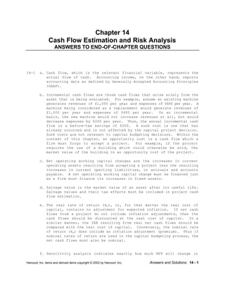
  • 17. Harcourt, Inc. items and derived items copyright © 2002 by Harcourt, Inc. Solution to Spreadsheet Problems: 14 - 17 If the actual life is 8 years: Amount Amount Year PV Factor before tax after tax Event Occurs at 10% PV Inflows: Revenues $10,000 $6,000 1-8 5.3349 $32,009 Depreciation 6,000 2,400 1-5 3.7908 9,098 Total PV of Inflows $41,107 NPV = $41,107 - $30,000 = $11,107. Alternatively, using a financial calculator, input the following: CF0 = -30000, CF1 = 8400, Nj = 5, CF4 = 6000, Nj = 3, and I = 10 to solve for NPV = $11,107.45 $11,107. If the life is as low as 4 years (an unlikely event), the investment will not be desirable. But, if the investment life is longer than 4 years, the investment will be a good one. Therefore, the decision will depend on the directors’ confidence in the life of the tractor. Given the low probability of the tractor’s life being only 4 years, it is likely that the directors will decide to purchase the tractor. b. 8% cost of capital; NPV = $3,539. 12% cost of capital; NPV = $280. NPV is still positive at a 12% cost of capital; therefore, the tractor should be purchased. The project is not very sensitive because when the cost of capital is increased by 4% NPV is still positive. c. At $7,000 operating revenue, NPV = ($4,981). At $13,000 operating revenue, NPV = $8,666. With a project life of one year, NPV = ($13,636). With a project life of ten years, NPV = $15,965. 4% cost of capital; NPV = $7,395. 16% cost of capital; NPV = ($2,496).
  • 18. Solution to Spreadsheet Problems: 14 - 18 Harcourt, Inc. items and derived items copyright © 2002 by Harcourt, Inc. NPV NPV (Thousandsof$) 10 8 5 3 1 (5) (3) 7 6 9 4 2 0 (6) (4) (2) (1) 7 9 Pre-tax Revenues (Thousands of $) 11 13 Sensitivity Diagram Sensitivity Diagram NPV vs. Project Life 15 10 20 5 0 (15) (10) (5) 97531 NPV (Thousandsof$) Project Life (Years) NPV NPV (Thousandsof$) Sensitivity Diagram NPV vs. Cost of Capital 7 5 9 3 1 (3) (2) (1) 6 4 8 2 0 1412 1610864 Cost of Capital (%) NPV
  • 19. Harcourt, Inc. items and derived items copyright © 2002 by Harcourt, Inc. Solution to Cyberproblem: 14 - 19 CYBERPROBLEM 14-15 The detailed solution for the cyberproblem is available on the instructor’s side of the Harcourt College Publishers’ web site: http://www.harcourtcollege.com/finance/theory10e.
  • 20. Mini Case: 14 - 20 Harcourt, Inc. items and derived items copyright © 2002 by Harcourt, Inc.