1. Scilab Textbook Companion for
Digital Signal Processing
by P. Ramesh Babu1
Created by
Mohammad Faisal Siddiqui
B.Tech (pursuing)
Electronics Engineering
Jamia Milia Islamia
College Teacher
Dr. Sajad A. Loan, JMI, New D
Cross-Checked by
Santosh Kumar, IITB
July 12, 2011
1
Funded by a grant from the National Mission on Education through ICT,
http://spoken-tutorial.org/NMEICT-Intro. This Textbook Companion and Scilab
codes written in it can be downloaded from the ”Textbook Companion Project”
section at the website http://scilab.in
2. Book Description
Title: Digital Signal Processing
Author: P. Ramesh Babu
Publisher: Scitech Publications (INDIA) Pvt. Ltd.
Edition: 4
Year: 2010
ISBN: 81-8371-081-7
1
3. Scilab numbering policy used in this document and the relation to the
above book.
Exa Example (Solved example)
Eqn Equation (Particular equation of the above book)
AP Appendix to Example(Scilab Code that is an Appednix to a particular
Example of the above book)
For example, Exa 3.51 means solved example 3.51 of this book. Sec 2.3 means
a scilab code whose theory is explained in Section 2.3 of the book.
2
4. Contents
List of Scilab Codes 4
1 DISCRETE TIME SIGNALS AND LINEAR SYSTEMS 11
2 THE Z TRANSFORM 34
3 THE DISCRETE FOURIER TRANSFORM 59
4 THE FAST FOURIER TRANSFORM 79
5 INFINITE IMPULSE RESPONSE FILTERS 90
6 FINITE IMPULSE RESPONSE FILTERS 102
7 FINITE WORD LENGTH EFFECTS IN DIGITAL FIL-
TERS 139
8 MULTIRATE SIGNAL PROCESSING 141
9 STATISTICAL DIGITAL SIGNAL PROCESSING 143
11 DIGITAL SIGNAL PROCESSORS 146
3
5. List of Scilab Codes
Exa 1.1 Continuous Time Plot and Discrete Time Plot . . . . 11
Exa 1.2 Continuous Time Plot and Discrete Time Plot . . . . 13
Exa 1.3.a Evaluate the Summations . . . . . . . . . . . . . . . . 14
Exa 1.3.b Evaluate the Summations . . . . . . . . . . . . . . . . 14
Exa 1.4.a Check for Energy or Power Signals . . . . . . . . . . . 15
Exa 1.4.d Check for Energy or Power Signals . . . . . . . . . . . 15
Exa 1.5.a Determining Periodicity of Signal . . . . . . . . . . . . 16
Exa 1.5.c Determining Periodicity of Signal . . . . . . . . . . . . 18
Exa 1.5.d Determining Periodicity of Signal . . . . . . . . . . . . 19
Exa 1.11 Stability of the System . . . . . . . . . . . . . . . . . 21
Exa 1.12 Convolution Sum of Two Sequences . . . . . . . . . . 21
Exa 1.13 Convolution of Two Signals . . . . . . . . . . . . . . . 22
Exa 1.18 Cross Correlation of Two Sequences . . . . . . . . . . 22
Exa 1.19 Determination of Input Sequence . . . . . . . . . . . . 23
Exa 1.32.a Plot Magnitude and Phase Response . . . . . . . . . . 24
Exa 1.37 Sketch Magnitude and Phase Response . . . . . . . . . 24
Exa 1.38 Plot Magnitude and Phase Response . . . . . . . . . . 26
Exa 1.45 Filter to Eliminate High Frequency Component . . . . 27
Exa 1.57.a Discrete Convolution of Sequences . . . . . . . . . . . 29
Exa 1.61 Fourier Transform . . . . . . . . . . . . . . . . . . . . 29
Exa 1.62 Fourier Transform . . . . . . . . . . . . . . . . . . . . 30
Exa 1.64.a Frequency Response of LTI System . . . . . . . . . . . 31
Exa 1.64.c Frequency Response of LTI System . . . . . . . . . . . 31
Exa 2.1 z Transform and ROC of Causal Sequence . . . . . . . 34
Exa 2.2 z Transform and ROC of Anticausal Sequence . . . . . 34
Exa 2.3 z Transform of the Sequence . . . . . . . . . . . . . . 35
Exa 2.4 z Transform and ROC of the Signal . . . . . . . . . . 36
Exa 2.5 z Transform and ROC of the Signal . . . . . . . . . . 36
4
6. Exa 2.6 Stability of the System . . . . . . . . . . . . . . . . . 37
Exa 2.7 z Transform of the Signal . . . . . . . . . . . . . . . . 37
Exa 2.8.a z Transform of the Signal . . . . . . . . . . . . . . . . 37
Exa 2.9 z Transform of the Sequence . . . . . . . . . . . . . . 38
Exa 2.10 z Transform Computation . . . . . . . . . . . . . . . . 38
Exa 2.11 z Transform of the Sequence . . . . . . . . . . . . . . 39
Exa 2.13.a z Transform of Discrete Time Signals . . . . . . . . . . 39
Exa 2.13.b z Transform of Discrete Time Signals . . . . . . . . . . 40
Exa 2.13.c z Transform of Discrete Time Signals . . . . . . . . . . 40
Exa 2.13.d z Transform of Discrete Time Signals . . . . . . . . . . 41
Exa 2.16 Impulse Response of the System . . . . . . . . . . . . 41
Exa 2.17 Pole Zero Plot of the Difference Equation . . . . . . . 42
Exa 2.19 Frequency Response of the System . . . . . . . . . . . 44
Exa 2.20.a Inverse z Transform Computation . . . . . . . . . . . 44
Exa 2.22 Inverse z Transform Computation . . . . . . . . . . . 45
Exa 2.23 Causal Sequence Determination . . . . . . . . . . . . . 45
Exa 2.34 Impulse Response of the System . . . . . . . . . . . . 46
Exa 2.35.a Pole Zero Plot of the System . . . . . . . . . . . . . . 47
Exa 2.35.b Unit Sample Response of the System . . . . . . . . . . 49
Exa 2.38 Determine Output Response . . . . . . . . . . . . . . 50
Exa 2.40 Input Sequence Computation . . . . . . . . . . . . . . 52
Exa 2.41.a z Transform of the Signal . . . . . . . . . . . . . . . . 53
Exa 2.41.b z Transform of the Signal . . . . . . . . . . . . . . . . 53
Exa 2.41.c z Transform of the Signal . . . . . . . . . . . . . . . . 54
Exa 2.45 Pole Zero Pattern of the System . . . . . . . . . . . . 55
Exa 2.53.a z Transform of the Sequence . . . . . . . . . . . . . . 55
Exa 2.53.b z Transform of the Signal . . . . . . . . . . . . . . . . 55
Exa 2.53.c z Transform of the Signal . . . . . . . . . . . . . . . . 56
Exa 2.53.d z Transform of the Signal . . . . . . . . . . . . . . . . 56
Exa 2.54 z Transform of Cosine Signal . . . . . . . . . . . . . . 56
Exa 2.58 Impulse Response of the System . . . . . . . . . . . . 58
Exa 3.1 DFT and IDFT . . . . . . . . . . . . . . . . . . . . . 59
Exa 3.2 DFT of the Sequence . . . . . . . . . . . . . . . . . . 60
Exa 3.3 8 Point DFT . . . . . . . . . . . . . . . . . . . . . . . 62
Exa 3.4 IDFT of the given Sequence . . . . . . . . . . . . . . . 62
Exa 3.7 Plot the Sequence . . . . . . . . . . . . . . . . . . . . 63
Exa 3.9 Remaining Samples . . . . . . . . . . . . . . . . . . . 64
Exa 3.11 DFT Computation . . . . . . . . . . . . . . . . . . . . 65
5
12. Chapter 1
DISCRETE TIME SIGNALS
AND LINEAR SYSTEMS
Scilab code Exa 1.1 Continuous Time Plot and Discrete Time Plot
1 //Example 1. 1
2 // S k et ch t he c o n ti n uo u s t im e s i g n a l x ( t ) =2∗exp(−2 t )
and a l so i t s d i s c r et e time e qu iv al en t s i g n al with
a s am pl in g p e r i od T = 0 . 2 s e c
3 clear all;
4 clc ;
5 close ;
6 t=0:0.01:2;
7 x1=2*exp (-2*t);
8 subplot(1,2,1);
9 plot(t,x1);
10 xlabel( ’ t ’ );
11 ylabel( ’ x ( t ) ’ );
12 title( ’CONTINUOUS TIME PLOT’ );
13 n=0:0.2:2;
14 x2=2*exp (-2*n);
15 subplot(1,2,2);
11
14. Figure 1.2: Continuous Time Plot and Discrete Time Plot
16 plot2d3(n,x2);
17 xlabel( ’ n ’ );
18 ylabel( ’x(n) ’ );
19 title( ’DISCRETE TIME PLOT ’ );
Scilab code Exa 1.2 Continuous Time Plot and Discrete Time Plot
1 //Example 1. 2
2 // S k et ch t he c o n ti n uo u s t im e s i g n a l x=s i n ( 7∗ t )+si n
(10∗ t ) and a l s o i t s d i s c r e t e time e q ui v a le n t
s i g n a l wi th a s am pl in g p e ri o d T = 0 . 2 s e c
13
15. 3 clear all;
4 clc ;
5 close ;
6 t=0:0.01:2;
7 x1=sin (7*t)+sin (10*t);
8 subplot(1,2,1);
9 plot(t,x1);
10 xlabel( ’ t ’ );
11 ylabel( ’ x ( t ) ’ );
12 title( ’CONTINUOUS TIME PLOT’ );
13 n=0:0.2:2;
14 x2=sin (7*n)+sin (10*n);
15 subplot(1,2,2);
16 plot2d3(n,x2);
17 xlabel( ’ n ’ );
18 ylabel( ’x(n) ’ );
19 title( ’DISCRETE TIME PLOT ’ );
Scilab code Exa 1.3.a Evaluate the Summations
1 //Example 1.3 (a )
2 //MAXIMA SCILAB TOOLBOX REQUIRED FOR THIS PROGRAM
3 // Calcu late Following Summations
4 clear all;
5 clc ;
6 close ;
7 syms n;
8 X = s ym su m (sin (2*n),n ,2, 2);
9 // Display the re su lt in command window
10 disp (X,”The Value of summation comes out to be : ”);
Scilab code Exa 1.3.b Evaluate the Summations
14
16. 1 //Example 1.3 (b)
2 //MAXIMA SCILAB TOOLBOX REQUIRED FOR THIS PROGRAM
3 // Calcu late Following Summations
4 clear all;
5 clc ;
6 close ;
7 syms n;
8 X= symsum (%e^(2*n),n ,0, 0);
9 // Display the re su lt in command window
10 disp (X,”The Value of summation comes out to be : ”);
Scilab code Exa 1.4.a Check for Energy or Power Signals
1 //Example 1.4 (a )
2 //MAXIMA SCILAB TOOLBOX REQUIRED FOR THIS PROGRAM
3 //Find Energy and Power of Given Sign als
4 clear all;
5 clc ;
6 close ;
7 syms n N ;
8 x=(1/3)^n;
9 E= symsum (x^2,n ,0, %inf);
10 // Display the re su lt in command window
11 disp (E,” Energy : ”);
12 p=(1/(2*N+1))*symsum (x^2,n ,0, N);
13 P=limit(p,N,%inf);
14 disp (P,”Power : ”);
15 // The E nergy i s F i n i t e and P ower i s 0 . T h e re f o re t he
g iv en s i g n a l i s an Energy S i gn a l
Scilab code Exa 1.4.d Check for Energy or Power Signals
1 //Example 1.4 (d)
15
17. 2 //MAXIMA SCILAB TOOLBOX REQUIRED FOR THIS PROGRAM
3 //Find Energy and Power of Given Sign als
4 clear all;
5 clc ;
6 close ;
7 syms n N ;
8 x=%e^(2*n);
9 E= symsum (x^2,n ,0, %inf);
10 // Display the re su lt in command window
11 disp (E,” Energy : ”);
12 p=(1/(2*N+1))*symsum (x^2,n ,0, N);
13 P=limit(p,N,%inf);
14 disp (P,”Power : ”);
15 //The Energy andPower i s i n f i n i t e . There fore the
g iv en s i g n a l i s an n e i th e r Energy S i gn a l nor
Power Sig nal
Scilab code Exa 1.5.a Determining Periodicity of Signal
1 //Example 1.5 (a )
2 //To Determine Whether Given Signal is Period ic or
not
3 clear all;
4 clc ;
5 close ;
6 t=0:0.01:2;
7 x1=exp(%i*6*%pi*t);
8 subplot(1,2,1);
9 plot(t,x1);
10 xlabel( ’ t ’ );
11 ylabel( ’ x ( t ) ’ );
12 title( ’CONTINUOUS TIME PLOT’ );
13 n=0:0.2:2;
16
19. Figure 1.4: Determining Periodicity of Signal
14 x2=exp(%i*6*%pi*n);
15 subplot(1,2,2);
16 plot2d3(n,x2);
17 xlabel( ’ n ’ );
18 ylabel( ’x(n) ’ );
19 title( ’DISCRETE TIME PLOT ’ );
20 //Hence Given Signal is Period ic with N=1
Scilab code Exa 1.5.c Determining Periodicity of Signal
1 //Example 1. 5 ( c )
18
20. 2 //To Determine Whether Given Signal is Period ic or
not
3 clear all;
4 clc ;
5 close ;
6 t=0:0.01:10;
7 x1=cos (2*%pi*t/3);
8 subplot(1,2,1);
9 plot(t,x1);
10 xlabel( ’ t ’ );
11 ylabel( ’ x ( t ) ’ );
12 title( ’CONTINUOUS TIME PLOT’ );
13 n=0:0.2:10;
14 x2=cos (2*%pi*n/3);
15 subplot(1,2,2);
16 plot2d3(n,x2);
17 xlabel( ’ n ’ );
18 ylabel( ’x(n) ’ );
19 title( ’DISCRETE TIME PLOT ’ );
20 //Hence Given Signal is Period ic with N=3
Scilab code Exa 1.5.d Determining Periodicity of Signal
1 //Example 1.5 (d)
2 //To Determine Whether Given Signal is Period ic or
not
3 clear all;
4 clc ;
5 close ;
6 t=0:0.01:50;
7 x1=cos(%pi*t/3)+cos (3*%pi*t/4);
8 subplot(1,2,1);
9 plot(t,x1);
19
22. 10 xlabel( ’ t ’ );
11 ylabel( ’ x ( t ) ’ );
12 title( ’CONTINUOUS TIME PLOT’ );
13 n=0:0.2:50;
14 x2=cos(%pi*n/3)+cos (3*%pi*n/4);
15 subplot(1,2,2);
16 plot2d3(n,x2);
17 xlabel( ’ n ’ );
18 ylabel( ’x(n) ’ );
19 title( ’DISCRETE TIME PLOT ’ );
20 //Hence Given Signal is Period ic with N=24
Scilab code Exa 1.11 Stability of the System
1 //Example 1.1 1
2 //MAXIMA SCILAB TOOLBOX REQUIRED FOR THIS PROGRAM
3 // T e st i ng S t a b i l i t y o f Given System
4 clear all;
5 clc ;
6 close ;
7 syms n;
8 x =(1/2)^n
9 X = s ym su m ( x, n ,0 , % in f ) ;
10 // Display the re su lt in command window
11 disp (X,”Summation i s : ”);
12 disp( ’ Hence Summation < i n f i n i t y . Given System i s
Stable ’ );
Scilab code Exa 1.12 Convolution Sum of Two Sequences
1 //Example 1.1 2
2 //Program to Compute convolution of given sequences
3 // x( n ) =[3 2 1 2 ] , h ( n) =[1 2 1 2 ] ;
21
23. 4 clear all;
5 clc ;
6 close ;
7 x = [3 2 1 2];
8 h = [1 2 1 2];
9 y=convol(x,h);
10 disp(y);
Scilab code Exa 1.13 Convolution of Two Signals
1 //Example 1.1 3
2 //Program to Compute convolution of given sequences
3 // x ( n ) =[1 2 1 1 ] , h ( n ) =[1 −1 1 −1];
4 clear all;
5 clc ;
6 close ;
7 x = [1 2 1 1];
8 h = [1 -1 1 -1];
9 y=convol(x,h);
10 disp(round(y));
Scilab code Exa 1.18 Cross Correlation of Two Sequences
1 //Example 1.1 8
2 //Program to Compute Cross−c o rr e la t i on o f given
sequences
3 // x( n ) =[1 2 1 1 ] , h ( n) =[1 1 2 1 ] ;
4 clear all;
5 clc ;
6 close ;
7 x = [1 2 1 1];
8 h = [1 1 2 1];
9 h1 =[1 2 1 1];
22
24. Figure 1.6: Plot Magnitude and Phase Response
10 y=convol(x,h1);
11 disp(round(y));
Scilab code Exa 1.19 Determination of Input Sequence
1 //Example 1.1 9
2 / /To f i n d i n pu t x ( n )
3 //h ( n) =[1 2 1 ] , y ( n) =[1 5 10 11 8 4 1 ]
4 clear all;
5 clc ;
6 close ;
7 z=%z;
8 a=z^6+5*(z^(5))+10*(z^(4))+11*(z^(3))+8*(z^(2))+4*(z
^(1))+1;
9 b=z^6+2*z^(5)+1*z^(4);
10 x =ldiv(a,b,5);
11 disp (x,”x(n)=”);
23
25. Scilab code Exa 1.32.a Plot Magnitude and Phase Response
1 //Example 1.3 2
2 //Program to Plot Magnitude and Phase Responce
3 clear all;
4 clc ;
5 close ;
6 w=-%pi:0.01:%pi;
7 H=1+2*cos(w)+2*cos(2*w);
8 // c a l u c u l a t i o n o f Pha se and Mag ni tud e o f H
9 [phase_H ,m]=phasemag (H);
10 Hm=abs(H);
11 a=gca ();
12 subplot(2,1,1);
13 a.y_location=” or ig in ”;
14 plot2d(w/%pi,Hm);
15 xlabel( ’ Frequency in Radians ’ )
16 ylabel( ’ abs (Hm) ’ );
17 title( ’MAGNITUDE RESPONSE ’ );
18 subplot(2,1,2);
19 a=gca ();
20 a.x_location=” or ig in ”;
21 a.y_location=” or ig in ”;
22 plot2d(w/(2*%pi),phase_H);
23 xlabel( ’ Frequency in Radians ’ );
24 ylabel( ’ <(H) ’ );
25 title( ’PHASE RESPONSE’ );
Scilab code Exa 1.37 Sketch Magnitude and Phase Response
24
26. Figure 1.7: Sketch Magnitude and Phase Response
1 //Example 1.3 7
2 //Program to Plot Magnitude and Phase Responce
3 //y( n) =1/2[x (n )+x( n−2) ]
4 clear all;
5 clc ;
6 close ;
7 w=0:0.01:%pi;
8 H=(1+cos(2*w)-%i*sin (2*w))/2;
9 // c a l u c u l a t i o n o f Pha se and Mag ni tud e o f H
10 [phase_H ,m]=phasemag (H);
11 Hm=abs(H);
12 a=gca ();
13 subplot(2,1,1);
14 a.y_location=” or ig in ”;
15 plot2d(w/%pi,Hm);
16 xlabel( ’ Frequency in Radians ’ )
17 ylabel( ’ abs (Hm) ’ );
18 title( ’MAGNITUDE RESPONSE ’ );
19 subplot(2,1,2);
20 a=gca ();
21 a.x_location=” or ig in ”;
22 a.y_location=” or ig in ”;
23 plot2d(w/(2*%pi),phase_H);
25
27. Figure 1.8: Plot Magnitude and Phase Response
24 xlabel( ’ Frequency in Radians ’ );
25 ylabel( ’ <(H) ’ );
26 title( ’PHASE RESPONSE’ );
Scilab code Exa 1.38 Plot Magnitude and Phase Response
1 //Example 1.3 8
2 //Program to Plot Magnitude and Phase Responce
3 // 0. 5 de lt a (n )+del ta (n−1)+0.5 de lt a (n−2)
4 clear all;
5 clc ;
6 close ;
7 w=-%pi:0.01:%pi;
8 H=0.5+exp(-%i*w)+0.5*exp(-%i*w);
9 // c a l u c u l a t i o n o f Pha se and Mag ni tud e o f H
10 [phase_H ,m]=phasemag (H);
11 Hm=abs(H);
12 a=gca ();
13 subplot(2,1,1);
26
28. 14 a.y_location=” or ig in ”;
15 plot2d(w/%pi,Hm);
16 xlabel( ’ Frequency in Radians ’ )
17 ylabel( ’ abs (Hm) ’ );
18 title( ’MAGNITUDE RESPONSE ’ );
19 subplot(2,1,2);
20 a=gca ();
21 a.x_location=” or ig in ”;
22 a.y_location=” or ig in ”;
23 plot2d(w/(2*%pi),phase_H);
24 xlabel( ’ Frequency in Radians ’ );
25 ylabel( ’ <(H) ’ );
26 title( ’PHASE RESPONSE’ );
Scilab code Exa 1.45 Filter to Eliminate High Frequency Component
1 //Example 1.4 5
2 //
3 clear all;
4 clc ;
5 close ;
6 t=0:0.01:10;
7 x=2*cos (5*t)+cos (300*t);
8 x1=2*cos (5*t);
9 b=[0.05 0.05];
10 a=[1 -0.9];
11 y=filter(b,a,x);
12 subplot(2,1,1);
13 plot(t,x);
14 xlabel( ’Time in Sec ’ );
15 ylabel( ’ Amplitud e ’ );
16 subplot(2,1,2);
17 plot(t,y);
27
30. 18 subplot(2,1,2);
19 plot(t,x1, ’ : ’ );
20 title( ’ x : SIGNAL WITHOUT NOISE y : SIGNAL WITH NOISE ’ )
;
21 xlabel( ’Time in Sec ’ );
22 ylabel( ’ Amplitud e ’ );
Scilab code Exa 1.57.a Discrete Convolution of Sequences
1 //Example 1.57 (a )
2 //Program to Compute di sc re te convolution of given
sequences
3 //x(n)=[1 2 −1 1 ] , h (n ) =[1 0 1 1 ] ;
4 clear all;
5 clc ;
6 close ;
7 x =[1 2 -1 1];
8 h = [1 0 1 1];
9 y=convol(x,h);
10 disp(round(y));
Scilab code Exa 1.61 Fourier Transform
1 //Example 1.6 1
2 //MAXIMA SCILAB TOOLBOX REQUIRED FOR THIS PROGRAM
3 // F o u r ie r t r an s fo r m o f ( 3 ) ˆ n u ( n )
4 clear all;
5 clc ;
6 close ;
7 syms n;
8 x = (3) ^ n;
9 X = s ym su m ( x, n ,0 , % in f )
10 // Display the re su lt in command window
29
31. Figure 1.10: Frequency Response of LTI System
11 disp (X,” The F o u r ie r T ra ns fo rm d oe s n ot e x i t a s x ( n )
is not abs olut ely summable and approaches
i n f i n i t y i . e . ”);
Scilab code Exa 1.62 Fourier Transform
1 //Example 1.6 2
2 //MAXIMA SCILAB TOOLBOX REQUIRED FOR THIS PROGRAM
3 // F o u r ie r t r an s fo r m o f ( 0 . 8 ) ˆ | n | u(n)
4 clear all;
5 clc ;
6 close ;
7 syms w n ;
8 X= symsum ((0.8)^n*%e^(%i*w*n),n ,1, %inf )+symsum
((0.8)^n*%e^(-%i*w*n),n ,0, %inf )
9 // Display the re su lt in command window
10 disp (X,”The Fourier Transform comes out to be : ”);
30
32. Scilab code Exa 1.64.a Frequency Response of LTI System
1 //Example 1.64 (a )
2 //Program to Calcu late Plot Magnitude and Phase
Responce
3 clear all;
4 clc ;
5 close ;
6 w=0:0.01:%pi;
7 H=1/(1-0.5*%e^(-%i*w));
8 // c a l u c u l a t i o n o f Pha se and Mag ni tud e o f H
9 [phase_H ,m]=phasemag (H);
10 Hm=abs(H);
11 a=gca ();
12 subplot(2,1,1);
13 a.y_location=” or ig in ”;
14 plot2d(w/%pi,Hm);
15 xlabel( ’ Frequency in Radians ’ )
16 ylabel( ’ abs (Hm) ’ );
17 title( ’MAGNITUDE RESPONSE ’ );
18 subplot(2,1,2);
19 a=gca ();
20 a.x_location=” or ig in ”;
21 a.y_location=” or ig in ”;
22 plot2d(w/(2*%pi),phase_H);
23 xlabel( ’ Frequency in Radians ’ );
24 ylabel( ’ <(H) ’ );
25 title( ’PHASE RESPONSE’ );
Scilab code Exa 1.64.c Frequency Response of LTI System
31
34. 1 //Example 1. 64 ( c )
2 //Program to Calcu late Plot Magnitude and Phase
Responce
3 clear all;
4 clc ;
5 close ;
6 w=0:0.01:%pi;
7 H=1/(1-0.9*%i*%e^(-%i*w));
8 // c a l u c u l a t i o n o f Pha se and Mag ni tud e o f H
9 [phase_H ,m]=phasemag (H);
10 Hm=abs(H);
11 a=gca ();
12 subplot(2,1,1);
13 a.y_location=” or ig in ”;
14 plot2d(w/%pi,Hm);
15 xlabel( ’ Frequency in Radians ’ )
16 ylabel( ’ abs (Hm) ’ );
17 title( ’MAGNITUDE RESPONSE ’ );
18 subplot(2,1,2);
19 a=gca ();
20 a.x_location=” or ig in ”;
21 a.y_location=” or ig in ”;
22 plot2d(w/(2*%pi),phase_H);
23 xlabel( ’ Frequency in Radians ’ );
24 ylabel( ’ <(H) ’ );
25 title( ’PHASE RESPONSE’ );
33
35. Chapter 2
THE Z TRANSFORM
Scilab code Exa 2.1 z Transform and ROC of Causal Sequence
1 //Example 2. 1
2 //Z− tr an sf or m o f [ 1 0 3 −1 2 ]
3 clear all;
4 clc ;
5 close ;
6 function[za]= ztransfer(sequence ,n)
7 z=poly (0, ’ z ’ , ’ r ’ )
8 za=sequence*(1/z)^n’
9 endfunction
10 x 1 =[1 0 3 -1 2];
11 n=0: length(x1)-1;
12 zz=ztransfer(x1,n);
13 // Display the re su lt in command window
14 disp (zz,”Z−t r an s f or m o f s e qu e nc e i s : ”);
15 disp( ’ROC i s t he e n t i r e p la ne e xc ep t z = 0 ’ );
Scilab code Exa 2.2 z Transform and ROC of Anticausal Sequence
34
36. 1 //Example 2. 2
2 //Z− t ra n sf or m o f [−3 −2 −1 0 1 ]
3 clear all;
4 clc ;
5 close ;
6 function[za]= ztransfer(sequence ,n)
7 z=poly (0, ’ z ’ , ’ r ’ )
8 za=sequence*(1/z)^n’
9 endfunction
10 x 1 =[ -3 -2 -1 0 1] ;
11 n=-(length(x1)-1):0;
12 zz=ztransfer(x1,n);
13 // Display the re su lt in command window
14 disp (zz,”Z−t r an s f or m o f s e qu e nc e i s : ”);
15 disp( ’ROC i s t he e n t i r e p l an e e x ce p t z = % i nf ’ );
Scilab code Exa 2.3 z Transform of the Sequence
1 //Example 2. 3
2 //Z− t ra n sf or m o f [ 2 −1 3 2 1 0 2 3 −1]
3 clear all;
4 clc ;
5 close ;
6 function[za]= ztransfer(sequence ,n)
7 z=poly (0, ’ z ’ , ’ r ’ )
8 za=sequence*(1/z)^n’
9 endfunction
10 x1 =[2 -1 3 2 1 0 2 3 -1];
11 n=-4:4;
12 zz=ztransfer(x1,n);
13 // Display the re su lt in command window
14 disp (zz,”Z−t r an s f or m o f s e qu e nc e i s : ”);
15 disp( ’ROC i s t he e n t i r e p la ne e xc ep t z = 0 and z =
%inf ’ );
35
37. Scilab code Exa 2.4 z Transform and ROC of the Signal
1 //Example 2. 4
2 //MAXIMA SCILAB TOOLBOX REQUIRED FOR THIS PROGRAM
3 //Z− tr a ns fo rm o f a ˆn u ( n )
4 clear all;
5 clc ;
6 close ;
7 syms a n z;
8 x = a^ n
9 X= symsum (x*(z^(-n)),n ,0, %inf );
10 // Display the re su lt in command window
11 disp (X,”Z−t r an s fo r m o f a ˆn u ( n ) w it h i s : ”);
12 disp( ’ROC i s the Region mod( z ) > a ’ )
Scilab code Exa 2.5 z Transform and ROC of the Signal
1 //Example 2. 5
2 //MAXIMA SCILAB TOOLBOX REQUIRED FOR THIS PROGRAM
3 //Z− tr a n sf o rm o f −bˆn u(−n−1)
4 clear all;
5 clc ;
6 close ;
7 syms b n z;
8 x = b^ n
9 X= symsum (x*(z^(-n)),n ,0, %inf );
10 // Display the re su lt in command window
11 disp (X,”Z−t r an s fo r m o f b ˆn u ( n ) w it h i s : ”);
12 disp( ’ROC i s the Region mod( z ) < b ’ )
36
38. Scilab code Exa 2.6 Stability of the System
1 //Example 2. 6
2 //MAXIMA SCILAB TOOLBOX REQUIRED FOR THIS PROGRAM
3 //Z− tr a ns fo rm o f 2ˆ n u ( n )
4 clear all;
5 clc ;
6 close ;
7 syms n z ;
8 x =(2) ^ n
9 X= symsum (x*(z^(-n)),n ,0, %inf );
10 // Display the re su lt in command window
11 disp (X,”Z−t ra ns fo rm o f 2ˆ n u ( n ) i s : ”);
12 disp( ’ROC i s the Region mod( z ) > 2 ’ );
Scilab code Exa 2.7 z Transform of the Signal
1 //Example 2. 7
2 //MAXIMA SCILAB TOOLBOX REQUIRED FOR THIS PROGRAM
3 //Z− t ra n sf or m o f [ 3 ( 3 ˆ n ) −4(2)ˆn ] u(n )
4 clear all;
5 clc ;
6 close ;
7 syms n z ;
8 x1 =(3) ^(n);
9 X1= symsum (3* x1 *(z^(-n)),n ,0, %inf );
10 x2 =(4) ^(n);
11 X2= symsum (4* x2 *(z^(-n)),n ,0, %inf );
12 X = ( X1 - X2 );
13 // Display the re su lt in command window
14 disp (X,”Z−t ra ns fo rm o f [ 3 ( 3 ˆ n ) −4(2) ˆn ] u ( n ) i s : ”);
Scilab code Exa 2.8.a z Transform of the Signal
37
39. 1 //Example 2.8 (a )
2 //MAXIMA SCILAB TOOLBOX REQUIRED FOR THIS PROGRAM
3 //Z transform of cos (Wo∗n )
4 clc;
5 syms Wo n z ;
6 x1=exp(sqrt(-1)*Wo*n);
7 X1=symsum(x1*(z^-n),n,0,%inf);
8 x2=exp(-sqrt(-1)*Wo*n);
9 X2=symsum(x2*(z^-n),n,0,%inf);
10 X=(X1+X2)/2;
11 disp(X, ’X( z )=’ );
Scilab code Exa 2.9 z Transform of the Sequence
1 //Example 2. 9
2 //MAXIMA SCILAB TOOLBOX REQUIRED FOR THIS PROGRAM
3 //Z− t r a ns f or m o f ( 1 / 3 )ˆ n u ( n−1)
4 clear all;
5 clc ;
6 close ;
7 syms n z ;
8 x =(1/3)^n;
9 X= (1/z)*symsum (x*(z^(-n)),n ,0, %inf );
10 // Display the re su lt in command window
11 disp (X,”Z−t r an s fo r m o f ( 1 / 3) ˆ n u ( n−1) is : ”);
Scilab code Exa 2.10 z Transform Computation
1 //Example 2.1 0
2 //MAXIMA SCILAB TOOLBOX REQUIRED FOR THIS PROGRAM
3 //Z trans form of rˆn . cos (Wo∗n )
4 clc;
5 syms r Wo n z;
38
40. 6 x1=(r^n)*exp(sqrt(-1)*Wo*n);
7 X1=symsum(x1*(z^-n),n,0,%inf);
8 x2=(r^n)*exp(-sqrt(-1)*Wo*n);
9 X2=symsum(x2*(z^-n),n,0,%inf);
10 X=(X1+X2)/2;
11 disp(X, ’X( z )=’ );
Scilab code Exa 2.11 z Transform of the Sequence
1 //Example 2.1 1
2 //MAXIMA SCILAB TOOLBOX REQUIRED FOR THIS PROGRAM
3 //Z− transform of n . aˆn u(n)
4 clear all;
5 clc ;
6 close ;
7 syms a n z;
8 x =( a) ^ n;
9 X= symsum (x*(z^(-n)),n ,0, %inf )
10 Y = diff (X,z);
11 // Display the re su lt in command window
12 disp (Y,”Z−t r an s fo r m o f n . a ˆn u ( n ) i s : ”);
Scilab code Exa 2.13.a z Transform of Discrete Time Signals
1 //Example 2.13 (a )
2 //MAXIMA SCILAB TOOLBOX REQUIRED FOR THIS PROGRAM
3 //Z− t ra n sf or m o f ( −1/5)ˆn u( n) +5(1/2)ˆ(−n)u(−n−1)
4 clear all;
5 clc ;
6 close ;
7 syms n z ;
8 x1 =(-1/5)^n ;
9 X1= symsum (x1 *(z^(-n)),n ,0, %inf );
39
41. 10 x2 =(1/2)^(-n);
11 X2= symsum (5* x2 *(z^(-n)),n ,0, %inf );
12 X = ( X1 - X2 );
13 // Display the re su lt in command window
14 disp (X,”Z−t ra ns fo rm o f [ 3 ( 3 ˆ n ) −4(2) ˆn ] u ( n ) i s : ”);
15 disp( ’ROC is the Region 1/5 < mod( z ) < 2 ’ );
Scilab code Exa 2.13.b z Transform of Discrete Time Signals
1 //Example 2.13 (b)
2 //MAXIMA SCILAB TOOLBOX REQUIRED FOR THIS PROGRAM
3 //Z transform
4 clc;
5 syms n z k;
6 x1=1;
7 X1=symsum(x1*z^(-n),n,0,0);
8 x2=1;
9 X2=symsum(x2*z^(-n),n,1,1);
10 x3=1;
11 X3=symsum(x3*z^(-n),n,2,2);
12 X=0.5*X1+X2-1/3*X3;
13 disp(X, ’X( z )=’ );
Scilab code Exa 2.13.c z Transform of Discrete Time Signals
1 //Example 2. 13 ( c )
2 //MAXIMA SCILAB TOOLBOX REQUIRED FOR THIS PROGRAM
3 //Z− tr a ns fo rm o f u ( n−2)
4 clear all;
5 clc ;
6 close ;
7 syms n z ;
8 x =1;
40
42. 9 X= (1/(z^2))*symsum (x*(z^(-n)),n ,0, %inf );
10 // Display the re su lt in command window
11 disp (X,”Z−t ra ns fo rm o f u ( n−2) is : ”);
Scilab code Exa 2.13.d z Transform of Discrete Time Signals
1 //Example 2.13 (d)
2 //MAXIMA SCILAB TOOLBOX REQUIRED FOR THIS PROGRAM
3 //Z− transform of (n+0.5) ((1/3) ˆn)u(n)
4 clear all;
5 clc ;
6 close ;
7 syms n z ;
8 x1 =(1/3)^n;
9 X11= symsum (x1*(z^(-n)),n ,0, %inf )
10 X1 = diff (X11,z);
11 x2 =(1/3) ^(n);
12 X2= symsum (0.5* x2 *(z^(-n)),n ,0, %inf );
13 X = ( X1 + X2 );
14 // Display the re su lt in command window
15 disp (X,”Z−t r an s fo r m o f ( n +0 .5 ) ( ( 1 / 3 ) ˆ n )u ( n ) i s : ”);
Scilab code Exa 2.16 Impulse Response of the System
1 //Example 2.1 6
2 / /To f i n d i n pu t h ( n )
3 //a=[1 2 −4 1 ] , b = [1 ]
4 clear all;
5 clc ;
6 close ;
7 z=%z;
8 a=z^3+2*(z^(2))-4*(z)+1;
9 b=z^3;
41
43. Figure 2.1: Pole Zero Plot of the Difference Equation
10 h =ldiv(a,b,4);
11 disp (h,”h(n)=”);
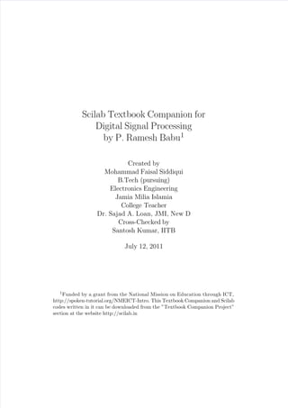
Scilab code Exa 2.17 Pole Zero Plot of the Difference Equation
1 //Example 2.1 7
2 //To draw the pole−z er o p l ot
3 clear all;
4 clc ;
5 close ;
6 z=%z
7 H1Z=((z)*(z-1))/((z-0.25)*(z-0.5));
8 xset( ’ window ’ ,1);
9 plzr(H1Z);
42
45. Scilab code Exa 2.19 Frequency Response of the System
1 //Example 2.1 9
2 //Program to Plot Magnitude and Phase Responce
3 clear all;
4 clc ;
5 close ;
6 w=-%pi:0.01:%pi;
7 H=1/(1-0.5*(cos(w)-%i*sin(w)));
8 // c a l u c u l a t i o n o f Pha se and Mag ni tud e o f H
9 [phase_H ,m]=phasemag (H);
10 Hm=abs(H);
11 a=gca ();
12 subplot(2,1,1);
13 a.y_location=” or ig in ”;
14 plot2d(w/%pi,Hm);
15 xlabel( ’ Frequency in Radians ’ );
16 ylabel( ’ abs (Hm) ’ );
17 title( ’MAGNITUDE RESPONSE ’ );
18 subplot(2,1,2);
19 a=gca ();
20 a.x_location=” or ig in ”;
21 a.y_location=” or ig in ”;
22 plot2d(w/(2*%pi),phase_H);
23 xlabel( ’ Frequency in Radians ’ );
24 ylabel( ’ <(H) ’ );
25 title( ’PHASE RESPONSE’ );
Scilab code Exa 2.20.a Inverse z Transform Computation
1 //Example 2.10 (a )
2 / /To f i n d i n pu t h ( n )
3 //X( z )=(z +0.2) / (( z +0. 5) ( z −1) ;
4 clear all;
5 clc ;
44
46. 6 close ;
7 z=%z;
8 a=(z+0.5)*(z-1);
9 b=z+0.2;
10 h =ldiv(b,a,4);
11 disp (h,”h(n)=”);
Scilab code Exa 2.22 Inverse z Transform Computation
1 //Example 2.2 2
2 / /To f i n d i n pu t x ( n )
3 //X( z ) =1/(2∗ z ˆ( −2)+2∗z ˆ( −1)+1) ;
4 clear all;
5 clc ;
6 close ;
7 z=%z;
8 a=(2+2*z+z^2);
9 b=z^2;
10 h =ldiv(b,a,6);
11 disp (h,” F i r s t s i x v a l ue s o f h ( n )=”);
Scilab code Exa 2.23 Causal Sequence Determination
1 //Example 2.2 3
2 / /To f i n d i n pu t x ( n )
3 //X( z ) =1/(1−2zˆ( −1))(1−z ˆ(−1)) ˆ2;
4 clear all;
5 clc ;
6 close ;
7 z=%z;
8 a=(z-2)*(z-1)^2;
9 b=z^3;
10 h =ldiv(b,a,6);
45
47. Figure 2.3: Impulse Response of the System
11 disp (h,” F i r s t s i x v a l ue s o f h ( n )=”);
Scilab code Exa 2.34 Impulse Response of the System
1 //Example 2.3 4
2 //To p l o t t he i m pu l se r e s po n c e o f t he s ys te m
a n a l y i c a l l y and u si ng s c i l a b
3 clear all;
4 clc ;
5 close ;
6 n=0:1:50;
46
48. 7 x=[1,zeros(1,50)];
8 b=[1 2];
9 a=[1 -3 -4];
10 yanaly=6/5*4.^n-1/5*(-1).^n;// A n a l y t i c a l S o l u t i o n
11 ymat=filter(b,a,x);
12 subplot(3,1,1);
13 plot2d3(n,x);
14 xlabel( ’ n ’ );
15 ylabel( ’x(n) ’ );
16 title( ’INPUT SEQUENCE (IMPULSE FUNCTION) ’ );
17 subplot(3,1,2);
18 plot2d3(n,yanaly);
19 xlabel( ’ n ’ );
20 ylabel( ’y(n) ’ );
21 title( ’OUTPUT SEQUENCE yanaly ’ );
22 subplot(3,1,3);
23 plot2d3(n,ymat);
24 xlabel( ’ n ’ );
25 ylabel( ’y(n) ’ );
26 title( ’OUTPUT SEQUENCE ymat ’ );
27 / /As t he A n a l t i c a l P lo t ma tches t he S c i l a b P lo t
h en ce i t i s t he Res pon ce o f t he s ys tem
Scilab code Exa 2.35.a Pole Zero Plot of the System
1 //Example 2.35 (a )
2 //To draw the pole−z er o p l ot
3 clear all;
4 clc ;
5 close ;
6 z=%z
7 H1Z=(z)/(z^2-z-1);
8 xset( ’ window ’ ,1);
47
50. Figure 2.5: Unit Sample Response of the System
9 plzr(H1Z);
Scilab code Exa 2.35.b Unit Sample Response of the System
1 //Example 2.35 (b)
2 //To p l o t t he r es p on ce o f t he s ys tem a n a l y i c a l l y and
u si ng s c i l a b
3 clear all;
4 clc ;
5 close ;
6 n=0:1:20;
49
51. 7 x=ones (1, length(n));
8 b=[0 1];
9 a=[1 -1 -1];
10 yanaly=0.447*(1.618).^n-0.447*(-0.618).^n;//
A n a l y ti c a l S o l u ti o n
11 [ymat,zf]=filter( b , a , x ) ;
12 subplot(3,1,1);
13 plot2d3(n,x);
14 xlabel( ’ n ’ );
15 ylabel( ’x(n) ’ );
16 title( ’INPUT SEQUENCE (STEP FUNCTION) ’ );
17 subplot(3,1,2);
18 plot2d3(n,yanaly);
19 xlabel( ’ n ’ );
20 ylabel( ’y(n) ’ );
21 title( ’OUTPUT SEQUENCE yanaly ’ );
22 subplot(3,1,3);
23 plot2d3(n,ymat,zf);
24 xlabel( ’ n ’ );
25 ylabel( ’y(n) ’ );
26 title( ’OUTPUT SEQUENCE ymat ’ );
27 / /As t he A n a l t i c a l P lo t ma tches t he S c i l a b P lo t
h en ce i t i s t he Res pon ce o f t he s ys tem
Scilab code Exa 2.38 Determine Output Response
1 //Example 2.3 8
2 //To p l o t t he r es p on ce o f t he s ys tem a n a l y i c a l l y and
u si ng s c i l a b
3 clear all;
4 clc ;
5 close ;
6 n=0:1:20;
50
53. 7 x=n;
8 b = [0 1 1];
9 a=[1 -0.7 0.12];
10 yanaly=38.89*(0.4).^n-26.53*(0.3).^n-12.36+4.76*n;//
A n a l y ti c a l S o l u ti o n
11 ymat=filter(b,a,x);
12 subplot(3,1,1);
13 plot2d3(n,x);
14 xlabel( ’ n ’ );
15 ylabel( ’x(n) ’ );
16 title( ’INPUT SEQUENCE (RAMP FUNCTION) ’ );
17 subplot(3,1,2);
18 plot2d3(n,yanaly);
19 xlabel( ’ n ’ );
20 ylabel( ’y(n) ’ );
21 title( ’OUTPUT SEQUENCE yanaly ’ );
22 subplot(3,1,3);
23 plot2d3(n,ymat);
24 xlabel( ’ n ’ );
25 ylabel( ’y(n) ’ );
26 title( ’OUTPUT SEQUENCE ymat ’ );
27 / /As t he A n a l t i c a l P lo t ma tches t he S c i l a b P lo t
h en ce i t i s t he Res pon ce o f t he s ys tem
Scilab code Exa 2.40 Input Sequence Computation
1 //Example 2.4 0
2 / /To f i n d i n pu t x ( n )
3 //h ( n)=1 2 3 2 , y ( n) =[1 3 7 10 10 7 2 ]
4 clear all;
5 clc ;
6 close ;
7 z=%z;
8 a=z^6+3*(z^(5))+7*(z^(4))+10*(z^(3))+10*(z^(2))+7*(z
^(1))+2;
52
54. 9 b=z^6+2*z^(5)+3*z^(4)+2*z^(3);
10 x =ldiv(a,b,4);
11 disp (x,”x(n)=”);
Scilab code Exa 2.41.a z Transform of the Signal
1 //Example 2.41 (a )
2 //MAXIMA SCILAB TOOLBOX REQUIRED FOR THIS PROGRAM
3 //Z− tr a ns fo rm o f n .( −1 ) ˆ n u ( n )
4 clear all;
5 clc ;
6 close ;
7 syms a n z;
8 x =( -1) ^ n;
9 X= symsum (x*(z^(-n)),n ,0, %inf )
10 Y = diff (X,z);
11 // Display the re su lt in command window
12 disp (Y,”Z−t ra ns fo rm o f n .( −1) ˆn u ( n ) i s : ”);
Scilab code Exa 2.41.b z Transform of the Signal
1 //Example 2.41 (b)
2 //MAXIMA SCILAB TOOLBOX REQUIRED FOR THIS PROGRAM
3 //Z− tr a ns fo rm o f n ˆ2 u ( n )
4 clear all;
5 clc ;
6 close ;
7 syms n z ;
8 x =1;
9 X= symsum (x*(z^(-n)),n ,0, %inf )
10 Y = diff(diff (X,z),z);
11 // Display the re su lt in command window
12 disp (Y,”Z−t ra ns fo rm o f n ˆ2 u ( n) i s : ”);
53
55. Figure 2.7: Pole Zero Pattern of the System
Scilab code Exa 2.41.c z Transform of the Signal
1 //Example 2. 41 ( c )
2 //MAXIMA SCILAB TOOLBOX REQUIRED FOR THIS PROGRAM
3 / /Z t ra ns fo r m o f (−1)ˆn . co s (%pi/3∗n )
4 clc;
5 syms n z ;
6 Wo=%pi/3;
7 x1=exp(sqrt(-1)*Wo*n);
8 X1=(-1)^n*symsum(x1*(z^-n),n,0,%inf);
9 x2=exp(-sqrt(-1)*Wo*n);
10 X2=(-1)^n*symsum(x2*(z^-n),n,0,%inf);
11 X=(X1+X2)/2;
12 disp(X, ’X( z )=’ );
54
56. Scilab code Exa 2.45 Pole Zero Pattern of the System
1 //Example 2.4 5
2 //To draw the pole−z er o p l ot
3 clear all;
4 clc ;
5 close ;
6 z=%z
7 H1Z=((z)*(z+1))/(z^2-z+0.5);
8 xset( ’ window ’ ,1);
9 plzr(H1Z);
Scilab code Exa 2.53.a z Transform of the Sequence
1 //Example 2.53 (a )
2 //Z− tra nsform o f [ 3 1 2 5 7 0 1 ]
3 clear all;
4 clc ;
5 close ;
6 function[za]= ztransfer(sequence ,n)
7 z=poly (0, ’ z ’ , ’ r ’ )
8 za=sequence*(1/z)^n’
9 endfunction
10 x1 =[3 1 2 5 7 0 1];
11 n=-3:3;
12 zz=ztransfer(x1,n);
13 // Display the re su lt in command window
14 disp (zz,”Z−t r an s f or m o f s e qu e nc e i s : ”);
Scilab code Exa 2.53.b z Transform of the Signal
1 //Example 2.53 (b)
2 //MAXIMA SCILAB TOOLBOX REQUIRED FOR THIS PROGRAM
55
57. 3 //Z t r an s fo r m o f d e l t a ( n )
4 clc;
5 syms n z ;
6 x=1;
7 X=symsum(x*z^(-n),n,0,0);
8 disp(X, ’X( z )=’ );
Scilab code Exa 2.53.c z Transform of the Signal
1 //Example 2. 53 ( c )
2 //MAXIMA SCILAB TOOLBOX REQUIRED FOR THIS PROGRAM
3 //Z t r an s fo r m o f d e l t a ( n )
4 clc;
5 syms n z k;
6 x=1;
7 X=symsum(x*z^(-n),n,k,k);
8 disp(X, ’X( z )=’ );
Scilab code Exa 2.53.d z Transform of the Signal
1 //Example 2.53 (d)
2 //MAXIMA SCILAB TOOLBOX REQUIRED FOR THIS PROGRAM
3 //Z t r an s fo r m o f d e l t a ( n )
4 clc;
5 syms n z kc ;
6 x=1;
7 X=symsum(x*z^(-n),n,-k,-k);
8 disp(X, ’X( z )=’ );
Scilab code Exa 2.54 z Transform of Cosine Signal
56
58. Figure 2.8: Impulse Response of the System
1 //Example 2.5 4
2 //MAXIMA SCILAB TOOLBOX REQUIRED FOR THIS PROGRAM
3 //Z transform of cos (Wo∗n )
4 clc;
5 syms Wo n z ;
6 x1=exp(sqrt(-1)*Wo*n);
7 X1=symsum(x1*(z^-n),n,0,%inf);
8 x2=exp(-sqrt(-1)*Wo*n);
9 X2=symsum(x2*(z^-n),n,0,%inf);
10 X=(X1+X2)/2;
11 disp(X, ’X( z )=’ );
57
59. Scilab code Exa 2.58 Impulse Response of the System
1 //Example 2.5 8
2 //To p l o t t he r es p on ce o f t he s ys tem a n a l y i c a l l y and
u si ng s c i l a b
3 clear all;
4 clc ;
5 close ;
6 n=0:1:20;
7 x=[1 zeros(1,20)];
8 b=[1 -0.5];
9 a=[1 -1 3/16];
10 yanaly=0.5*(0.75).^n+0.5*(0.25).^n;// Ana lyti cal
S o l u t i o n
11 ymat=filter(b,a,x);
12 subplot(3,1,1);
13 plot2d3(n,x);
14 xlabel( ’ n ’ );
15 ylabel( ’x(n) ’ );
16 title( ’INPUT SEQUENCE (IMPULSE FUNCTION) ’ );
17 subplot(3,1,2);
18 plot2d3(n,yanaly);
19 xlabel( ’ n ’ );
20 ylabel( ’y(n) ’ );
21 title( ’OUTPUT SEQUENCE yanaly ’ );
22 subplot(3,1,3);
23 plot2d3(n,ymat);
24 xlabel( ’ n ’ );
25 ylabel( ’y(n) ’ );
26 title( ’OUTPUT SEQUENCE ymat ’ );
27 / /As t he A n a l t i c a l P lo t ma tches t he S c i l a b P lo t
h en ce i t i s t he Res pon ce o f t he s ys tem
58
60. Chapter 3
THE DISCRETE FOURIER
TRANSFORM
Scilab code Exa 3.1 DFT and IDFT
1 //Example 3. 1
2 //Program to Compute the DFT of a Sequence x [ n
]=[ 1 ,1 ,0 ,0 ]
3 //and IDFT of a Sequence Y[ k ]= [1 ,0 ,1 ,0 ]
4 clear all;
5 clc ;
6 close ;
7 x = [1,1,0,0];
8 //DFT Computation
9 X = fft ( x , -1) ;
10 Y = [1,0,1,0];
11 //IDFT Computation
12 y = fft ( Y , 1 ) ;
13 // Dis pla y sequ ence X[ k ] and y [ n ] in command window
14 disp(X,”X[ k]= ”);
15 disp(y,”y [ n]=”);
59
61. Figure 3.1: DFT of the Sequence
Scilab code Exa 3.2 DFT of the Sequence
1 //Example 3. 2
2 //Program to Compute the DFT of a Sequence x [ n]=1 ,
0<=n<=2; and 0 otherwise
3 // fo r N=4 and N=8. Plot Magnitude and phase pl ots of
each .
4 clear all;
5 clc ;
6 close ;
7 //N=4
8 x1 = [1,1,1,0];
9 //DFT Computation
10 X1 = fft ( x1 , -1) ;
11 //N=8
12 x2 = [1,1,1,0,0,0,0,0];
13 //DFT Computation
14 X2 = fft ( x2 , -1) ;
15 // Dis pla y sequ ence X1 [ k ] and X2 [ k ] in command window
16 disp(X1,”X1 [ k]=” );
60
62. 17 disp(X2,”X2 [ k]=” );
18 // Plots for N=4
19 n1=0:1:3;
20 subplot(2,2,1);
21 a = gca ();
22 a.y_location =” or ig in ”;
23 a.x_location =” or ig in ”;
24 plot2d3(n1,abs(X1),2);
25 poly1=a.children(1).children (1);
26 poly1.thickness=2;
27 xtitle( ’N=4 ’ , ’ k ’ , ’ | X1(k) | ’ );
28 subplot(2,2,2);
29 a = gca ();
30 a.y_location =” or ig in ”;
31 a.x_location =” or ig in ”;
32 plot2d3(n1,atan(imag(X1),real(X1)),5);
33 poly1=a.children(1).children (1);
34 poly1.thickness=2;
35 xtitle( ’N=4 ’ , ’ k ’ , ’<X1( k) ’ );
36 // Plots for N=8
37 n2=0:1:7;
38 subplot(2,2,3);
39 a = gca ();
40 a.y_location =” or ig in ”;
41 a.x_location =” or ig in ”;
42 plot2d3(n2,abs(X2),2);
43 poly1=a.children(1).children (1);
44 poly1.thickness=2;
45 xtitle( ’N=8 ’ , ’ k ’ , ’ | X2(k) | ’ );
46 subplot(2,2,4);
47 a = gca ();
48 a.y_location =” or ig in ”;
49 a.x_location =” or ig in ”;
50 plot2d3(n2,atan(imag(X2),real(X2)),5);
51 poly1=a.children(1).children (1);
52 poly1.thickness=2;
53 xtitle( ’N=8 ’ , ’ k ’ , ’<X2( k) ’ );
61
63. Scilab code Exa 3.3 8 Point DFT
1 //Example 3. 3
2 //Program to Compute the 8−point DFT o f the Sequence
x [ n ]= [1 ,1 , 1 ,1 ,1 ,1 ,0 ,0 ]
3 clear all;
4 clc ;
5 close ;
6 x = [1,1,1,1,1,1,0,0];
7 //DFT Computation
8 X = fft ( x , -1) ;
9 // Dis pla y sequ ence X[ k ] in command window
10 disp(X,”X[ k]= ”);
Scilab code Exa 3.4 IDFT of the given Sequence
1 //Example 3. 4
2 //Program to Compute the IDFT of the Sequence X[ k
]=[ 5 ,0 ,1 − j ,0 ,1 ,0 ,1 + j , 0 ]
3 clear all;
4 clc ;
5 close ;
6 j=sqrt (-1);
7 X = [5,0,1-j,0,1,0,1+j,0]
8 //IDFT Computation
9 x = fft ( X , 1 ) ;
10 // Di sp la y se qu en ce s x [ n ] in command window
11 disp(x,”x [ n]=”);
62
64. Figure 3.2: Plot the Sequence
Scilab code Exa 3.7 Plot the Sequence
1 //Example 3. 7
2 //Program to Compute ci rc ul ar convolution of
f o l l o w i n g s e qu e nc es
3 //x [ n ]= [1 ,2 ,2 ,1 ,0 ]
4 //Y[ k]= exp(− j ∗4∗ pi ∗k /5 ) .X[ k ]
5 clear all;
6 clc ;
7 close ;
8 x=[1,2,2,1,0];
9 X=fft(x,-1);
10 k=0:1:4;
11 j=sqrt (-1);
12 pi=22/7;
63
65. 13 H=exp(-j*4*pi*k/5);
14 Y=H.*X;
15 //IDFT Computation
16 y=fft(Y,1);
17 // Dis pla y sequ ence y [ n ] in command window
18 disp(round(y),”y [ n]=”);
19 // Pl ot s
20 n=0:1:4;
21 a = gca ();
22 a.y_location =” or ig in ”;
23 a.x_location =” or ig in ”;
24 plot2d3(n,round(y),5);
25 poly1=a.children(1).children (1);
26 poly1.thickness=2;
27 xtitle( ’ Plot of sequence y [ n ] ’ , ’ n ’ , ’ y [n ] ’ );
Scilab code Exa 3.9 Remaining Samples
1 //Example 3. 9
2 //Program to remaining samples of the sequence
3 //X(0 ) =12,X(1)=−1+j3 , X(2 )=3+j4 , X(3 )=1−j5 ,X(4 )=−2+j2 ,
X(5 )=6+j3 ,X( 6) =−2−j3 ,X(7 ) =10
4 clear all;
5 clc ;
6 close ;
7 j=sqrt (-1);
8 z=1;
9 X(0+z)=12,X(1+z)=-1+j*3,X(2+z)=3+j*4,X(3+z)=1-j*5,X
(4+z)=-2+j*2,X(5+z)=6+j*3,X(6+z)=-2-j*3,X(7+z)
=10;
10 for a=9:1:14 do X(a)=conj(X(16-a)), end;
11 // Displa y the complete sequence X[ k ] in command
window
12 disp(X,”X[ k]= ”);
64
66. Scilab code Exa 3.11 DFT Computation
1 //Example 3.1 1
2 //Program to Compute the 8−point DFT of the
f o l l o w i n g s e qu e nc es
3 //x1 [ n ]= [1 ,0 ,0 ,0 ,0 ,1 ,1 ,1]
4 //x2 [ n ]= [0 ,0 ,1 ,1 ,1 ,1 ,0 ,0]
5 clear all;
6 clc ;
7 close ;
8 x1=[1,0,0,0,0,1,1,1];
9 x2=[0,0,1,1,1,1,0,0];
10 //DFT Computation
11 X1 = fft ( x1 , -1) ;
12 X2 = fft ( x2 , -1) ;
13 // Displa y sequ ences X1[ k ] and X2[ k ] in command
window
14 disp(X1,”X1 [ k]=” );
15 disp(X2,”X2 [ k]=” );
Scilab code Exa 3.13 Circular Convolution
1 //Example 3.1 3
2 //Program to Compute ci rc ul ar convolution of
f o l l o w i n g s e qu e nc es
3 //x1 [ n]=[1 , −1 , −2 , 3 , −1]
4 //x2 [ n ]= [1 ,2 ,3 ]
5 clear all;
6 clc ;
7 close ;
8 x1=[1,-1,-2,3,-1];
9 x2=[1,2,3];
65
67. 10 / /Loop f o r z er o p add in g t he s m a l l er s eq ue nc e o ut o f
the two
11 n1=length(x1);
12 n2=length(x2);
13 n3=n2-n1;
14 if (n3>=0) then
15 x1=[x1,zeros(1,n3)];
16 else
17 x2=[x2,zeros(1,-n3)];
18 end
19 //DFT Computation
20 X1=fft(x1,-1);
21 X2=fft(x2,-1);
22 Y=X1.*X2;
23 //IDFT Computation
24 y=fft(Y,1);
25 // Dis pla y sequ ence y [ n ] in command window
26 disp(y,”y [ n]=”);
Scilab code Exa 3.14 Circular Convolution
1 //Example 3.1 4
2 //Program to Compute ci rc ul ar convolution of
f o l l o w i n g s e qu e nc es
3 //x1 [ n ]= [1 ,2 ,2 ,1 ]
4 //x2 [ n ]= [1 ,2 ,3 ,1 ]
5 clear all;
6 clc ;
7 close ;
8 x1=[1,2,2,1];
9 x2=[1,2,3,1];
10 //DFT Computation
11 X1=fft(x1,-1);
12 X2=fft(x2,-1);
13 Y=X1.*X2;
66
68. 14 //IDFT Computation
15 y=fft(Y,1);
16 // Dis pla y sequ ence y [ n ] in command window
17 disp(y,”y [ n]=”);
Scilab code Exa 3.15 Determine Sequence x3
1 //Example 3.1 5
2 // Program to Compute x3 [ n ] where X3 [ k]=X1 [ k ] . X2 [ k ]
3 //x1 [ n ]= [1 ,2 ,3 ,4 ]
4 //x2 [ n ]= [1 ,1 ,2 ,2 ]
5 clear all;
6 clc ;
7 close ;
8 x1=[1,2,3,4];
9 x2=[1,1,2,2];
10 //DFT Computation
11 X1=fft(x1,-1);
12 X2=fft(x2,-1);
13 X3=X1.*X2;
14 //IDFT Computation
15 x3=fft(X3,1);
16 // Dis pla y sequ ence x3 [ n ] in command window
17 disp(x3,”x3 [ n]=” );
Scilab code Exa 3.16 Circular Convolution
1 //Example 3.1 6
2 //Program to Compute ci rc ul ar convolution of
f o l l o w i n g s e qu e nc es
3 //x1 [ n ]= [1 ,1 ,2 ,1 ]
4 //x2 [ n ]= [1 ,2 ,3 ,4 ]
5 clear all;
67
69. 6 clc ;
7 close ;
8 x1=[1,1,2,1];
9 x2=[1,2,3,4];
10 //DFT Computation
11 X1=fft(x1,-1);
12 X2=fft(x2,-1);
13 X3=X1.*X2;
14 //IDFT Computation
15 x3=fft(X3,1);
16 // Dis pla y sequ ence x3 [ n ] in command window
17 disp(x3,”x3 [ n]=” );
Scilab code Exa 3.17 Circular Convolution
1 //Example 3.1 7
2 // Program to Compute y [ n ] where Y[ k]=X1 [ k ] . X2 [ k ]
3 //x1 [ n ]= [0 ,1 ,2 ,3 ,4 ]
4 //x2 [ n ]= [0 ,1 ,0 ,0 ,0 ]
5 clear all;
6 clc ;
7 close ;
8 x1=[0,1,2,3,4];
9 x2=[0,1,0,0,0];
10 //DFT Computation
11 X1=fft(x1,-1);
12 X2=fft(x2,-1);
13 Y=X1.*X2;
14 //IDFT Computation
15 y=round(fft(Y,1));
16 // Dis pla y sequ ence y [ n ] in command window
17 disp(y,”y [ n]=”);
68
70. Scilab code Exa 3.18 Output Response
1 //Example 3.1 8
2 //Program to Compute output responce of fol low ing
sequences
3 //x [ n ]= [1 ,2 ,3 ,1 ]
4 //h [ n ]= [1 ,1 ,1 ]
5 // (1) Linear Convolution
6 // (2) Circ ula r Convolution
7 // (3) Circula r Convolution with zero padding
8 clear all;
9 clc ;
10 close ;
11 x=[1,2,3,1];
12 h=[1,1,1];
13 // (1) Linear Convolution Computation
14 ylinear=convol (x,h);
15 // Displa y Linear Convoluted Sequence y [ n ] in command
window
16 disp(yli near ,” yl in ea r [ n]=”);
17 // (2) Circ ula r Convolution Computation
18 //Now zero padding in h [ n ] sequence to make length
of x [ n ] and h [ n ] equal
19 h1=[h,zeros(1,1)];
20 //Now Performing Cir cu la r Convolution by DFT method
21 X=fft(x,-1);
22 H=fft(h1,-1);
23 Y=X.*H;
24 ycircular=fft(Y,1);
25 // Display Circ ula r Convoluted Sequence y [ n ] in
command window
26 disp(ycircular ,” yc ir cu la r [ n]=”);
27 // (3) Circ ula r Convolution Computation with zero
Padding
28 x2=[x,zeros(1,2)];
29 h2=[h,zeros(1,3)];
30 //Now Performing Cir cu la r Convolution by DFT method
31 X2=fft(x2,-1);
69
71. 32 H2=fft(h2,-1);
33 Y2=X2.*H2;
34 ycircularp=fft(Y2,1);
35 // Display Circula r Convoluted Sequence with zero
Padding y [ n ] in command window
36 disp(ycircularp ,” yc ir cu la rp [ n]=”);
Scilab code Exa 3.20 Output Response
1 //Example 3.2 0
2 //Program to Compute Linear Convolution of fol low ing
sequences
3 //x [ n ]= [3 , − 1 ,0 ,1 ,3 ,2 ,0 ,1 ,2 ,1 ]
4 //h [ n ]= [1 ,1 ,1 ]
5 clear all;
6 clc ;
7 close ;
8 x=[3,-1,0,1,3,2,0,1,2,1];
9 h=[1,1,1];
10 // Linear Convolution Computation
11 y=convol (x,h);
12 // Dis pla y Sequence y [ n ] in command window
13 disp(y,”y [ n]=”);
Scilab code Exa 3.21 Linear Convolution
1 //Example 3.2 1
2 //Program to Compute Linear Convolution of fol low ing
sequences
3 //x [ n]=[ 1 ,2 , −1 ,2 ,3 , −2 , −3 , −1 ,1 ,1 ,2 , −1]
4 //h [ n ]= [1 ,2]
5 clear all;
6 clc ;
70
72. 7 close ;
8 x=[1,2,-1,2,3,-2,-3,-1,1,1,2,-1];
9 h=[1,2];
10 // Linear Convolution Computation
11 y=convol (x,h);
12 // Dis pla y Sequence y [ n ] in command window
13 disp(y,”y [ n]=”);
Scilab code Exa 3.23.a N Point DFT Computation
1 //Example 3.23 (a )
2 //MAXIMA SCILAB TOOLBOX REQUIRED FOR THIS PROGRAM
3 //N point DFT of del ta (n)
4 clc;
5 syms n k N;
6 x=1;
7 X=symsum(x*exp(-%i*2*%pi*n*k/N),n,0,0);
8 disp(X, ’X( k)=’ );
Scilab code Exa 3.23.b N Point DFT Computation
1 //Example 3.23 (b)
2 //MAXIMA SCILAB TOOLBOX REQUIRED FOR THIS PROGRAM
3 //N point DFT of del ta (n−no )
4 clc;
5 syms n k N no ;
6 x=1;
7 X=symsum(x*exp(-%i*2*%pi*n*k/N),n,-no,-no);
8 disp(X, ’X( k)=’ );
71
73. Scilab code Exa 3.23.c N Point DFT Computation
1 //Example 3. 23 ( c )
2 //MAXIMA SCILAB TOOLBOX REQUIRED FOR THIS PROGRAM
3 //N point DFT of aˆn
4 clc;
5 syms a n k N ;
6 x=a^n;
7 X=symsum(x*exp(-%i*2*%pi*n*k/N),n,0,N-1);
8 disp(X, ’X( k)=’ );
Scilab code Exa 3.23.d N Point DFT Computation
1 //Example 3.23 (d)
2 //MAXIMA SCILAB TOOLBOX REQUIRED FOR THIS PROGRAM
3 //N point DFT of x(n) =1, 0<=n<
=N/2−1
4 clc;
5 syms n k N;
6 x=1;
7 X=symsum(x*exp(-%i*2*%pi*n*k/N),n,0,(N/2)-1);
8 disp(X, ’X( k)=’ );
Scilab code Exa 3.23.e N Point DFT Computation
1 //Example 3. 23 ( e )
2 //MAXIMA SCILAB TOOLBOX REQUIRED FOR THIS PROGRAM
3 //N poi nt DFT of x( n)=exp(%i∗2∗%pi∗ko∗n/N) ;
4 clc;
5 syms n k N ko ;
6 x=exp(%i*2*%pi*ko*n/N);
7 X=symsum(x*exp(-%i*2*%pi*n*k/N),n,0,(N/2)-1);
8 disp(X, ’X( k)=’ );
72
74. Scilab code Exa 3.23.f N Point DFT Computation
1 //Example 3.2 3 ( f )
2 //MAXIMA SCILAB TOOLBOX REQUIRED FOR THIS PROGRAM
3 //N point DFT of x(n) =1, for n=even and 0 , for n=odd
4 clc;
5 syms n k N ;
6 x=1; // x (2 n ) =1 , f o r a l l n
7 X=symsum(x*exp(-%i*4*%pi*n*k/N),n,0,N/2-1);
8 disp(X, ’X( k)=’ );
Scilab code Exa 3.24 DFT of the Sequence
1 //Example 3.2 4
2 //Program to Compute the DFT of the Sequence x [ n
]=( −1)ˆn , fo r N=4
3 clear all;
4 clc ;
5 close ;
6 N=4;
7 n=0:1:N-1;
8 x=(-1)^n;
9 //DFT Computation
10 X = fft (x,-1);
11 // Dis pla y Sequence X[ k ] in command window
12 disp(X,”X[ k]= ”);
Scilab code Exa 3.25 8 Point Circular Convolution
73
75. 1 //Example 3.2 5
2 //Program to Compute the 8−p o in t C i r c ul a r
Convolution of the Sequences
3 //x1 [ n ]= [1 ,1 ,1 ,1 ,0 ,0 ,0 ,0]
4 // x2 [ n]= s i n (3 ∗ p i ∗n/8)
5 clear all;
6 clc ;
7 close ;
8 x1=[1,1,1,1,0,0,0,0];
9 n=0:1:7;
10 pi=22/7;
11 x2=sin (3*pi*n/8);
12 //DFT Computation
13 X1=fft (x1,-1);
14 X2=fft (x2,-1);
15 // Circ ula r Convolution using DFT
16 Y=X1.*X2;
17 //IDFT Computation
18 y= fft (Y,1);
19 // Dis pla y sequ ence y [ n ] in command window
20 disp(y,”y [ n]=”);
Scilab code Exa 3.26 Linear Convolution using DFT
1 //Example 3.2 6
2 //Program to Compute the Linear Convolution of the
f o l l o w i n g S eq ue nc es
3 //x [ n ]= [1 , −1 ,1]
4 //h [ n ]= [2 ,2 ,1 ]
5 clear all;
6 clc ;
7 close ;
8 x=[1,-1,1];
9 h=[2,2,1];
10 // Convol ution Computation
74
76. 11 y= convol(x,h);
12 // Dis pla y sequ ence y [ n ] in command window
13 disp(y,”y [ n]=”);
Scilab code Exa 3.27.a Circular Convolution Computation
1 //Example 3.27 (a )
2 //Program to Compute the Convolution of the
f o l l o w i n g S eq ue nc es
3 //x1 [ n ]= [1 ,1 ,1 ]
4 // x2 [ n ]= [2 , −1 ,2 ]
5 clear all;
6 clc ;
7 close ;
8 x1=[1,1,1];
9 x2=[2,-1,2];
10 // Convol ution Computation
11 X1=fft (x1,-1);
12 X2=fft (x2,-1);
13 Y=X1.*X2;
14 y=fft (Y,1);
15 // Dis pla y Sequence y [ n ] in command window
16 disp(y,”y [ n]=”);
Scilab code Exa 3.27.b Circular Convolution Computation
1 //Example 3.27 (b)
2 //Program to Compute the Convolution of the
f o l l o w i n g S eq ue nc es
3 // x1 [ n]=[1 ,1 , −1 , −1 ,0 ]
4 // x2 [ n ]= [1 ,0 , − 1 ,0 ,1 ]
5 clear all;
6 clc ;
75
77. 7 close ;
8 x1=[1,1,-1,-1,0];
9 x2=[1,0,-1,0,1];
10 // Convol ution Computation
11 X1=fft (x1,-1);
12 X2=fft (x2,-1);
13 Y=X1.*X2;
14 y= fft (Y,1);
15 // Dis pla y Sequence y [ n ] in command window
16 disp(y,”y [ n]=”);
Scilab code Exa 3.30 Calculate value of N
1 //Example 3.3 0
2 //Program to Calculate N from given data
3 //fm=5000Hz
4 // df=50Hz
5 // t =0.5 se c
6 clear all;
7 clc ;
8 close ;
9 fm=5000 //Hz
10 df=50 //Hz
11 t=0.5 // se c
12 N1=2*fm/df;
13 N=2;
14 while N<=N1, N=N*2,end
15 // Displ aying the value of N in command window
16 disp(N,”N=”);
Scilab code Exa 3.32 Sketch Sequence
76
78. Figure 3.3: Sketch Sequence
1 //Example 3.3 2
2 // Program t o p l o t t he r e s u l t o f t he g i ve n s eq ue nc e
3 //X[ k ]= [1 ,2 ,2 ,1 ,0 ,2 ,1 ,2 ]
4 //y [ n]=x [ n /2 ] fo r n=even ,0 fo r n=odd
5 clear all;
6 clc ;
7 close ;
8 X=[1,2,2,1,0,2,1,2];
9 x = fft ( X , 1 ) ;
10 y=[x(1),0,x(2),0,x(3),0,x(4),0,x(5),0,x(6),0,x(7),0,
x(8) ,0];
11 Y = fft ( y , -1) ;
12 // Dis pla y sequ ence Y[ k ] and in command window
13 disp(Y,”Y[ k]= ”);
14 // Plotti ng the sequence Y[ k ]
15 k=0:1:15;
16 a = gca ();
17 a.y_location =” or ig in ”;
18 a.x_location =” or ig in ”;
19 plot2d3(k,Y,2);
20 poly1=a.children(1).children (1);
21 poly1.thickness=2;
22 xtitle( ’ Plot of Y(k) ’ , ’ k ’ , ’Y(k ) ’ );
77
79. Scilab code Exa 3.36 Determine IDFT
1 //Example 3.3 6
2 //Program to Compute the IDFT of the fol lo wi ng
Sequence
3 //X[ k]=[12 , −1.5 + j2 .598 , −1.5 + j0 .866 ,0 ,−1.5 − j 0
.866, −1.5 − j 2 . 5 9 8 ]
4 clear all;
5 clc ;
6 close ;
7 j=sqrt (-1);
8 X=[12,-1.5+j*2.598,-1.5+j*0.866,0,-1.5-j*0.866,-1.5-
j*2.598];
9 //IDFT Computation
10 x = fft ( X , 1 ) ;
11 // Dis pla y Sequence x [ n ] in command window
12 disp(round(x),”x [ n]=”);
78
80. Chapter 4
THE FAST FOURIER
TRANSFORM
Scilab code Exa 4.3 Shortest Sequence N Computation
1 //Example 4. 3
2 // Program t o c a l c u l a t e s h o r t e s t s eq ue nc e N su ch t ha t
a l go r it h m B r un s // f a s t e r than A
3 clear all;
4 clc ;
5 close ;
6 i=0;
7 N=32; //Given
8 / / C a l c u l a t i o n o f T wi dd le f a c t o r e xp o ne nt s f o r e ac h
stage
9 while 1==1
10 i=i+1;
11 N=2^i;
12 A=N^2;
13 B=5*N*log2(N);
14 if A>B then break;
15 end;
16 end
17 disp(N, ’SHORTEST SEQUENCE N =’ );
79
81. Scilab code Exa 4.4 Twiddle Factor Exponents Calculation
1 //Example 4. 4
2 // Program t o c a l c u l a t e T wi dd le f a c t o r e xp o ne nt s f o r
e ac h s t a g e
3 clear all;
4 clc ;
5 close ;
6 N=32; //Given
7 / / C a l c u l a t i o n o f T wi dd le f a c t o r e xp o ne nt s f o r e ac h
stage
8 for m=1:5
9 disp(m, ’ Stage : m = ’ );
10 disp( ’ k = ’);
11 for t=0:(2^(m-1)-1)
12 k=N*t/2^m;
13 disp(k);
14 end
15 end
Scilab code Exa 4.6 DFT using DIT Algorithm
1 //Example 4. 6
2 //Program to fin d the DFT of a Sequence x [ n
]= [1 ,2 ,3 ,4 ,4 ,3 ,2 ,1]
3 // usi ng DIT Algorithm .
4 clear all;
5 clc ;
6 close ;
7 x = [1,2,3,4,4,3,2,1];
8 //FFT Computation
80
82. 9 X = fft ( x , -1) ;
10 disp(X, ’X( z ) = ’ );
Scilab code Exa 4.8 DFT using DIF Algorithm
1 //Example 4. 8
2 //Program to fin d the DFT of a Sequence x [ n
]= [1 ,2 ,3 ,4 ,4 ,3 ,2 ,1]
3 // usi ng DIF Algorithm .
4 clear all;
5 clc ;
6 close ;
7 x = [1,2,3,4,4,3,2,1];
8 //FFT Computation
9 X = fft ( x , -1) ;
10 disp(X, ’X( z ) = ’ );
Scilab code Exa 4.9 8 Point DFT of the Sequence
1 //Example 4. 9
2 / / Program t o f i n d t he 8−point DFT of a Sequence x [ n
]=1 , 0<=n<=7
3 // usi ng DIT , DIF Algorithm .
4 clear all;
5 clc ;
6 close ;
7 x = [1,1,1,1,1,1,1,1];
8 //FFT Computation
9 X = fft ( x , -1) ;
10 disp(X, ’X( z ) = ’ );
81
83. Scilab code Exa 4.10 4 Point DFT of the Sequence
1 //Example 4.1 0
2 //Program to Compute the 4−point DFT of a Sequence x
[ n ]= [0 ,1 ,2 ,3]
3 // usi ng DIT−DIF Algorithm .
4 clear all;
5 clc ;
6 close ;
7 x = [0,1,2,3];
8 //FFT Computation
9 X = fft ( x , -1) ;
10 disp(X, ’X( z ) = ’ );
Scilab code Exa 4.11 IDFT of the Sequence using DIT Algorithm
1 //Example 4.1 1
2 //Program to Compute the IDFT of a Sequence using
DIT Algo rithm .
3 //X[ k ] = [7, −0.707 − j0 .707 , − j ,0.707 − j0 .707 ,1 ,0. 707 + j0
.7 0 7 , j ,−0.707+ j0 .7 0 7 ]
4 clear all;
5 clc ;
6 close ;
7 j=sqrt (-1);
8 X = [7,-0.707-j *0.707,-j ,0.707-j*0.707 ,1,0.707+j
*0.707,j,-0.707+j*0.707];
9 // In ve rs e FFT Computation
10 x = fft ( X , 1 ) ;
11 disp(x, ’ x( n) = ’ );
Scilab code Exa 4.12 8 Point DFT of the Sequence
82
84. 1 //Example 4.1 2
2 //Program to Compute the 8−point DFT of a Sequence
3 //x [ n ]=[ 0. 5 ,0 .5 ,0. 5 ,0 .5 ,0 ,0 ,0 ,0 ] using radix−2 DIT
Algor ithm .
4 clear all;
5 clc ;
6 close ;
7 x=[0.5,0.5,0.5,0.5,0,0,0,0];
8 //FFT Computation
9 X = fft ( x , -1) ;
10 disp(X, ’X( z ) = ’ );
Scilab code Exa 4.13 8 Point DFT of the Sequence
1 //Example 4.1 3
2 //Program to Compute the 8−point DFT of a Sequence
3 //x [ n ]=[ 0. 5 ,0 .5 ,0. 5 ,0 .5 ,0 ,0 ,0 ,0 ] using radix−2 DIF
Algor ithm .
4 clear all;
5 clc ;
6 close ;
7 x=[0.5,0.5,0.5,0.5,0,0,0,0];
8 //FFT Computation
9 X = fft ( x , -1) ;
10 disp(X, ’X( z ) = ’ );
Scilab code Exa 4.14 DFT using DIT Algorithm
1 //Example 4.1 4
2 //Program to Compute the 4−point DFT of a Sequence x
[ n]=[ 1 , −1 ,1 , −1]
3 // usi ng DIT Algorithm .
4 clear all;
83
85. 5 clc ;
6 close ;
7 x=[1,-1,1,-1];
8 //FFT Computation
9 X =fft ( x , -1) ;
10 disp(X, ’X( z ) = ’ );
Scilab code Exa 4.15 DFT using DIF Algorithm
1 //Example 4.1 5
2 //Program to Compute the 4−point DFT of a Sequence x
[ n ]= [1 ,0 ,0 ,1]
3 // usi ng DIF Algorithm .
4 clear all;
5 clc ;
6 close ;
7 x=[1,0,0,1];
8 //FFT Computation
9 X =fft ( x , -1) ;
10 disp(X, ’X( z ) = ’ );
Scilab code Exa 4.16.a 8 Point DFT using DIT FFT
1 //Example 4.16 (a )
2 //Program to Evaluate and Compare the 8−poin t DFT of
the given Sequence
3 // x1 [ n]=1 , −3<=n<=3 usi ng DIT−FFT Alg ori thm .
4 clear all;
5 clc ;
6 close ;
7 x1=[1,1,1,1,0,1,1,1];
8 //FFT Computation
9 X1 = fft ( x1 , -1) ;
84
86. 10 disp(X1, ’ X1 ( k ) = ’ );
Scilab code Exa 4.16.b 8 Point DFT using DIT FFT
1 //Example 4.16 (b)
2 //Program to Evaluate and Compare the 8−poin t DFT of
the given Sequence
3 //x2 [ n]=1 , 0<=n<=6 using DIT−FFT Alg ori thm .
4 clear all;
5 clc ;
6 close ;
7 x2=[1,1,1,1,1,1,1,0];
8 //FFT Computation
9 X2 = fft ( x2 , -1) ;
10 disp(X2, ’ X2 ( k ) = ’ );
Scilab code Exa 4.17 IDFT using DIF Algorithm
1 //Example 4.1 7
2 //Program to find the IDFT of the Sequence using DIF
Algorithm .
3 //X[ k]= [4 ,1 − j2 .4 14 ,0 ,1 − j0 .4 14 ,0 ,1 + j0 .414 ,0 ,1+ j2
. 4 1 4 ]
4 clear all;
5 clc ;
6 close ;
7 j=sqrt (-1);
8 X= [4,1-j*2.414,0,1-j*0.414,0 ,1+j*0.414,0 ,1+j
*2.414];
9 // In ve rs e FFT Computation
10 x = fft ( X , 1 ) ;
11 disp(x, ’ x( n) = ’ );
85
87. Scilab code Exa 4.18 IDFT using DIT Algorithm
1 //Example 4.1 8
2 //Program to fin d the IDFT of the Sequence X[ k]=
[10,−2+j2 ,−2,−2− j2 ]
3 // usi ng DIT Algorithm .
4 clear all;
5 clc ;
6 close ;
7 j=sqrt (-1);
8 X = [10,-2+j*2,-2,-2-j*2];
9 // In ve rs e FFT Computation
10 x = fft ( X , 1 ) ;
11 disp(x, ’ x( n) = ’ );
Scilab code Exa 4.19 FFT Computation of the Sequence
1 //Example 4.1 9
2 //Program to Compute the FFT of given Sequence x [ n
]= [1 ,0 ,0 ,0 ,0 ,0 ,0 ,0 ].
3 clear all;
4 clc ;
5 close ;
6 x = [1,0,0,0,0,0,0,0];
7 //FFT Computation
8 X = fft ( x , -1) ;
9 disp(X, ’X( z ) = ’ );
Scilab code Exa 4.20 8 Point DFT by Radix 2 DIT FFT
86
88. 1 //Example 4.2 0
2 //Program to Compute the 8−point DFT o f given
Sequence
3 //x [ n ]=[2 ,2 ,2 ,2 ,1 ,1 ,1 ,1] using DIT, radix −2,FFT
Algor ithm .
4 clear all;
5 clc ;
6 close ;
7 x = [2,2,2,2,1,1,1,1];
8 //FFT Computation
9 X = fft ( x , -1) ;
10 disp(X, ’X( z ) = ’ );
Scilab code Exa 4.21 DFT using DIT FFT Algorithm
1 //Example 4.2 1
2 //Program to Compute the DFT of given Sequence
3 //x [ n]=[1 , −1 , −1 , −1 ,1 ,1 ,1 , −1] using DIT−FFT Algo rithm
.
4 clear all;
5 clc ;
6 close ;
7 x = [1,-1,-1,-1,1,1,1,-1];
8 //FFT Computation
9 X = fft ( x , -1) ;
10 disp(X, ’X( z ) = ’ );
Scilab code Exa 4.22 Compute X using DIT FFT
1 //Example 4.2 2
2 //Program to Compute the DFT of given Sequence
3 //x [ n]=2ˆn and N=8 us in g DIT−FFT Alg ori thm .
4 clear all;
87
89. 5 clc ;
6 close ;
7 N=8;
8 n=0:1:N-1;
9 x =2^n;
10 //FFT Computation
11 X = fft ( x , -1) ;
12 disp(X, ’X( z ) = ’ );
Scilab code Exa 4.23 DFT using DIF FFT Algorithm
1 //Example 4.2 3
2 //Program to Compute the DFT of given Sequence
3 //x [ n]= co s (n∗ pi /2) , and N=4 usi ng DIF−FFT Alg ori thm .
4 clear all;
5 clc ;
6 close ;
7 N=4;
8 pi=22/7;
9 n=0:1:N-1;
10 x =cos(n*pi/2);
11 //FFT Computation
12 X = fft ( x , -1) ;
13 disp(X, ’X( z ) = ’ );
Scilab code Exa 4.24 8 Point DFT of the Sequence
1 //Example 4.2 4
2 //Program to Compute the 8−point DFT o f given
Sequence
3 //x [ n ]=[ 0 ,1 ,2 ,3 ,4 ,5 ,6 ,7 ] usin g DIF , radix −2,FFT
Algor ithm .
4 clear all;
88
90. 5 clc ;
6 close ;
7 x = [0,1,2,3,4,5,6,7];
8 //FFT Computation
9 X = fft ( x , -1) ;
10 disp(X, ’X( z ) = ’ );
89
91. Chapter 5
INFINITE IMPULSE
RESPONSE FILTERS
Scilab code Exa 5.1 Order of the Filter Determination
1 //Example 5. 1
2 //To Find out the order of the f i l t e r
3 clear all;
4 clc ;
5 close ;
6 ap=1; //db
7 as=30;//db
8 op=200; //rad/ sec
9 os=600; //rad/ sec
10 N=log(sqrt ((10^(0.1*as)-1)/(10^(0.1*ap)-1)))/log(os/
op);
11 disp(ceil (N), ’ Order of the f i l t e r , N =’ );
Scilab code Exa 5.2 Order of Low Pass Butterworth Filter
1 //Example 5. 2
90
92. 2 //To Find out the order of a Low Pass Butterworth
F i l t e r
3 clear all;
4 clc ;
5 close ;
6 ap=3; //db
7 as=40;//db
8 fp=500; //Hz
9 fs=1000; //Hz
10 op=2*%pi*fp;
11 os=2*%pi*fs;
12 N=log(sqrt ((10^(0.1*as)-1)/(10^(0.1*ap)-1)))/log(os/
op);
13 disp(ceil (N), ’ Order of the f i l t e r , N =’ );
Scilab code Exa 5.4 Analog Butterworth Filter Design
1 //Example 5. 4
2 //To Design an Analog Butterworth Fi lt er
3 clear all;
4 clc ;
5 close ;
6 ap=2; //db
7 as=10;//db
8 op=20;//rad/ sec
9 os=30;//rad/ sec
10 N=log(sqrt ((10^(0.1*as)-1)/(10^(0.1*ap)-1)))/log(os/
op);
11 disp(ceil (N), ’ Order of the f i l t e r , N =’ );
12 s=%s;
13 HS=1/((s^2+0.76537*s+1)*(s^2+1.8477*s+1));// Tran sfer
Function fo r N=4
14 oc=op/(10^(0.1*ap)-1)^(1/(2*ceil(N)));
15 HS1=horner(HS,s/oc);
16 disp(HS1, ’ Normalized Tran sfer Function , H( s ) =’ );
91
93. Scilab code Exa 5.5 Analog Butterworth Filter Design
1 //Example 5. 5
2 //To Design an Analog Butterworth Fi lt er
3 clear all;
4 clc ;
5 close ;
6 op=0.2*%pi;
7 os=0.4*%pi;
8 e1=0.9;
9 l1=0.2;
10 epsilon=sqrt(1/(e1^2)-1);
11 lambda=sqrt (1/(l1^2)-1);
12 N=log(lambda/epsilon)/log(os/op);
13 disp(ceil (N), ’ Order of the f i l t e r , N =’ );
14 s=%s;
15 HS=1/((s^2+0.76537*s+1)*(s^2+1.8477*s+1));// Tran sfer
Function fo r N=4
16 oc=op/epsilon^(1/ceil(N));
17 HS1=horner(HS,s/oc);
18 disp(HS1, ’ Normalized Tran sfer Function , H( s ) =’ );
Scilab code Exa 5.6 Order of Chebyshev Filter
1 //Example 5. 6
2 / /To Find out th e o rd er o f t he F i l t e r u si ng
Chebyshev Approximation
3 clear all;
4 clc ;
5 close ;
6 ap=3; //db
92
94. 7 as=16;//db
8 fp=1000; //Hz
9 fs=2000; //Hz
10 op=2*%pi*fp;
11 os=2*%pi*fs;
12 N=acosh(sqrt ((10^(0.1*as)-1)/(10^(0.1*ap)-1)))/acosh
(os/op);
13 disp(ceil (N), ’ Order of the f i l t e r , N =’ );
Scilab code Exa 5.7 Chebyshev Filter Design
1 //Example 5. 7
2 //To Design an analog Chebyshev Fi lt er with Given
S p e c i f i c a t i o n s
3 clear all;
4 clc ;
5 close ;
6 os=2;
7 op=1;
8 ap=3; //db
9 as=16;//db
10 e1=1/ sqrt (2);
11 l1=0.1;
12 epsilon=sqrt(1/(e1^2)-1);
13 lambda=sqrt (1/(l1^2)-1);
14 N=acosh(lambda/epsilon)/acosh(os/op);
15 disp(ceil (N), ’ Order of the f i l t e r , N =’ );
Scilab code Exa 5.8 Order of Type 1 Low Pass Chebyshev Filter
1 //Example 5. 8
2 / /To Find o ut t he o r de r o f t he p o l e s o f t he Type 1
Lowpass Chebyshev Fi lt er
93
95. 3 clear all;
4 clc ;
5 close ;
6 ap=1; //dB
7 as=40;//dB
8 op=1000*%pi;
9 os=2000*%pi;
10 N=acosh(sqrt ((10^(0.1*as)-1)/(10^(0.1*ap)-1)))/acosh
(os/op);
11 disp(ceil (N), ’ Order of the f i l t e r , N =’ );
Scilab code Exa 5.9 Chebyshev Filter Design
1 //Example 5. 9
2 //To Design a Chebyshev Fi lt er with Given
S p e c i f i c a t i o n s
3 clear all;
4 clc ;
5 close ;
6 ap=2.5; //db
7 as=30;//db
8 op=20;//rad/ sec
9 os=50;//rad/ sec
10 N=acosh(sqrt ((10^(0.1*as)-1)/(10^(0.1*ap)-1)))/acosh
(os/op);
11 disp(ceil (N), ’ Order of the f i l t e r , N =’ );
Scilab code Exa 5.10 HPF Filter Design with given Specifications
1 //Example 5.1 0
2 / /To D es ig n a H. P . F. wi th g i ve n s p e c i f i c a t i o n s
3 clear all;
4 clc ;
94
96. 5 close ;
6 ap=3; //db
7 as=15;//db
8 op=500; //rad/ sec
9 os=1000; //rad/ sec
10 N=log(sqrt ((10^(0.1*as)-1)/(10^(0.1*ap)-1)))/log(os/
op);
11 disp(ceil (N), ’ Order of the f i l t e r , N =’ );
12 s=%s;
13 HS=1/((s+1)*(s^2+s+1));// Transfer Function for N=3
14 oc=1000 //rad/ sec
15 HS1=horner(HS,oc/s);
16 disp(HS1, ’ Normalized Tran sfer Function , H( s ) =’ );
Scilab code Exa 5.11 Impulse Invariant Method Filter Design
1 //Example 5.1 1
2 / /To D e si gn t he F i l t e r u s in g I mp ul se I n v a r i e nt
Method
3 clear all;
4 clc ;
5 close ;
6 s=%s;
7 T=1;
8 HS=(2)/(s^2+3*s+2);
9 elts=pfss (HS);
10 disp(elts, ’ Factorized HS = ’ );
11 / /The p o l e s comes o ut t o be a t −2 and −1
12 p1=-2;
13 p2=-1;
14 z=%z;
15 HZ=(2/(1-%e^(p2*T)*z^(-1)))-(2/(1-%e^(p1*T)*z^(-1)))
16 disp(HZ, ’HZ = ’ );
95
97. Scilab code Exa 5.12 Impulse Invariant Method Filter Design
1 //Example 5.1 2
2 //MAXIMA SCILAB TOOLBOX REQUIRED FOR THIS PROGRAM
3 / /To D e si gn t he F i l t e r u s in g I mp ul se I n v a r i e nt
Method
4 clear all;
5 clc ;
6 close ;
7 s=%s;
8 HS=1/(s^2+sqrt (2)*s+1);
9 pp=ilaplace(HS);
10 syms n z ;
11 t=1;
12 X= symsum (pp*(z^(-n)),n ,0, %inf );
13 disp(X, ’ Factorized HS = ’ );
Scilab code Exa 5.13 Impulse Invariant Method Filter Design
1 //Example 5.1 3
2 //MAXIMA SCILAB TOOLBOX REQUIRED FOR THIS PROGRAM
3 / /To D es ig n t he 3 r d Order B ut te rw or th F i l t e r u s i ng
Impulse Inv ari ent Method
4 clear all;
5 clc ;
6 close ;
7 s=%s;
8 HS=1/((s+1)*(s^2+s+1));
9 pp=ilaplace(HS);// Inverse Laplace
10 syms n z ;
11 t=1;
12 X= symsum (pp*(z^(-n)),n ,0, %inf );//Z Transform
96
98. 13 disp(X, ’H( z )= ’ );
Scilab code Exa 5.15 Impulse Invariant Method Filter Design
1 //Example 5.1 5
2 / /To D e si gn t he F i l t e r u s in g I mp ul se I n v a r i e nt
Method
3 clear all;
4 clc ;
5 close ;
6 s=%s;
7 T=0.2;
8 HS=10/(s^2+7*s+10);
9 elts=pfss (HS);
10 disp(elts, ’ Factorized HS = ’ );
11 / /The p o l e s comes o ut t o be a t −5 and −2
12 p1=-5;
13 p2=-2;
14 z=%z;
15 HZ=T*((-3.33/(1-%e^(p1*T)*z^(-1)))+(3.33/(1-%e^(p2*T
)*z^(-1))))
16 disp(HZ, ’HZ = ’ );
Scilab code Exa 5.16 Bilinear Transformation Method Filter Design
1 //Example 5.1 6
2 //To Find out Bi li ne ar Transformation of HS=2/(( s+1)
∗( s +2) )
3 clear all;
4 clc ;
5 close ;
6 s=%s;
7 z=%z;
97
99. 8 HS=2/((s+1)*(s+2));
9 T=1;
10 HZ=horner(HS,(2/T)*(z-1)/(z+1));
11 disp(HZ, ’H( z ) =’ );
Scilab code Exa 5.17 HPF Design using Bilinear Transform
1 //Example 5.1 7
2 //To Design an H.P.F. monotonic in passband using
Bil ine ar Transform
3 clear all;
4 clc ;
5 close ;
6 ap=3; //db
7 as=10;//db
8 fp=1000; //Hz
9 fs=350; //Hz
10 f=5000;
11 T=1/f;
12 wp=2*%pi*fp;
13 ws=2*%pi*fs;
14 op=2/T*tan(wp*T/2);
15 os=2/T*tan(ws*T/2);
16 N=log(sqrt ((10^(0.1*as)-1)/(10^(0.1*ap)-1)))/log(op/
os);
17 disp(ceil (N), ’ Order of the f i l t e r , N =’ );
18 s=%s;
19 HS=1/(s+1)// Transfer Function for N=1
20 oc=op//rad/ sec
21 HS1=horner(HS,oc/s);
22 disp(HS1, ’ Normalized Tran sfer Function , H( s ) =’ );
23 z=%z;
24 HZ=horner(HS,(2/T)*(z-1)/(z+1));
25 disp(HZ, ’H( z ) =’ );
98
100. Scilab code Exa 5.18 Bilinear Transformation Method Filter Design
1 //Example 5.1 8
2 //To Find out Bil ine ar Transformation of H( s )=(s
ˆ2+4 .525 ) /( s ˆ2+0.692∗ s +0.50 4)
3 clear all;
4 clc ;
5 close ;
6 s=%s;
7 z=%z;
8 HS=(s^2+4.525)/(s^2+0.692*s+0.504);
9 T=1;
10 HZ=horner(HS,(2/T)*(z-1)/(z+1));
11 disp(HZ, ’H( z ) =’ );
Scilab code Exa 5.19 Single Pole LPF into BPF Conversion
1 //Example 5.1 9
2 //To Convert a si ng le Pole LPF into BPF
3 clear all;
4 clc ;
5 close ;
6 s=%s;
7 z=%z;
8 HZ=(0.5*(1+z^(-1)))/(1-0.302*z^(-2));
9 T=1;
10 wu=3*%pi/4;
11 wl=%pi/4;
12 wp=%pi/6;
13 k=tan(wp/2)/tan ((wu-wl)/2);
14 a=cos ((wu+wl)/2)/cos((wu-wl)/2);
99
101. 15 transf=-((((k-1)/(k+1))*(z^(-2)))-((2*a*k/(k+1))*(z
^(-1)))+1)/(z^( -2) -(2*a*k/(1+k)*z ^(-1))+((k-1)/(k
+1)));
16 HZ1=horner(HZ,transf);
17 disp(HZ1, ’H( z ) of B.P.F =’ );
Scilab code Exa 5.29 Pole Zero IIR Filter into Lattice Ladder Structure
1 //Example 5.2 9
2 //Program to convert given IIR pole−z er o F i l t e r i nt o
L a t t i c e La dd er S t r u c t ur e .
3 clear all;
4 clc ;
5 close ;
6 U=1; //Zero Adjust
7 a(3+U,0+U)=1;
8 a(3+U,1+U)=13/24;
9 a(3+U,2+U)=5/8;
10 a(3+U,3+U)=1/3;
11 a(2+U,0+U)=1; //a(m,0)=1
12 a(2+U,3+U)=1/3;
13 m=3,k=1;
14 a(m-1+U,k+U)=(a(m+U,k+U)-a(m+U,m+U)*a(m+U,m-k+U))
/(1-a(m+U,m+U)*a(m+U,m+U));
15 m=3,k=2;
16 a(m-1+U,k+U)=(a(m+U,k+U)-a(m+U,m+U)*a(m+U,m-k+U))
/(1-a(m+U,m+U)*a(m+U,m+U));
17 m=2,k=1;
18 a(m-1+U,k+U)=(a(m+U,k+U)-a(m+U,m+U)*a(m+U,m-k+U))
/(1-a(m+U,m+U)*a(m+U,m+U));
19 disp( ’LATTICE COEFFICIENTS ’ );
20 disp(a(1+U,1+U), ’ k1 ’ );
21 disp(a(2+U,2+U), ’ k2 ’ );
22 disp(a(3+U,3+U), ’ k3 ’ );
23 b0=1;
100
109. 8 N=11;
9 U=6;
10 for n=-5+U:1:5+U
11 if n==6
12 hd(n)=0.5;
13 else
14 hd(n)=(sin(%pi*3*(n-U)/4)-sin(%pi*(n-U)/4))/(%pi*(n-
U));
15 end
16 end
17 [ hzm , fr ]= frmag (hd ,256) ;
18 hzm_dB = 20* log10 (hzm)./ max ( h z m ) ;
19 figure
20 plot ( 2* fr , h zm _d B )
21 a= gca ();
22 xlabel ( ’ Frequency w∗ pi ’ );
23 ylabel ( ’ Magnitude in dB ’ );
24 title ( ’ Frequency Response of FIR BPF with N=11 ’ );
25 xgrid (2);
Scilab code Exa 6.8 BRF Magnitude Response
1 //Example 6. 8
2 //Program to Plot Magnitude Responce of id eal B.R.F.
with
3 //wc1=0.33∗ pi and wc2=0.67∗ p i
4 //N=11
5 clear all;
6 clc ;
7 close ;
8 N=11;
9 U=6;
10 for n=-5+U:1:5+U
108
111. 11 if n==6
12 hd(n)=0.5;
13 else
14 hd(n)=(sin(%pi*(n-U))+sin(%pi*(n-U)/3)-sin(%pi*2*(n-
U)/3))/(%pi*(n-U));
15 end
16 end
17 [ hzm , fr ]= frmag (hd ,256) ;
18 hzm_dB = 20* log10 (hzm)./ max ( h z m ) ;
19 figure
20 plot ( 2* fr , h zm _d B )
21 a= gca ();
22 xlabel ( ’ Frequency w∗ pi ’ );
23 ylabel ( ’ Magnitude in dB ’ );
24 title ( ’ Frequency Response of FIR BRF with N=11 ’ );
25 xgrid (2);
Scilab code Exa 6.9.a HPF Magnitude Response using Hanning Window
1 //Example 6. 9 a
2 //Program to Plot Magnitude Responce of id eal H.P.F.
3 // us in g Hanning Window
4 //wc1=0.25∗ pi
5 //N=11
6 clear all;
7 clc ;
8 close ;
9 N=11;
10 U=6;
11 h_hann=window( ’ hn ’ ,N);
12 for n=-5+U:1:5+U
13 if n==6
14 hd(n)=0.75;
110
112. Figure 6.5: HPF Magnitude Response using Hanning Window
111
113. 15 else
16 hd(n)=(sin(%pi*(n-U))-sin(%pi*(n-U)/4))/(%pi*(n-U));
17 end
18 h(n)=h_hann(n)*hd(n);
19 end
20 [ hzm , fr ]= frmag ( h ,256) ;
21 hzm_dB = 20* log10 (hzm)./ max ( h z m ) ;
22 figure
23 plot ( 2* fr , h zm _d B )
24 a= gca ();
25 xlabel ( ’ Frequency w∗ pi ’ );
26 ylabel ( ’ Magnitude in dB ’ );
27 title ( ’ Frequency Response of FIR HRF with N=11
us in g Hanning Window ’);
28 xgrid (2);
Scilab code Exa 6.9.b HPF Magnitude Response using Hamming Win-
dow
1 //Example 6.9 b
2 //Program to Plot Magnitude Responce of id eal H.P.F.
3 // using Hamming Window
4 //wc1=0.25∗ pi
5 //N=11
6 clear all;
7 clc ;
8 close ;
9 N=11;
10 U=6;
11 h_hamm=window( ’hm ’ ,N);
12 for n=-5+U:1:5+U
13 if n==6
14 hd(n)=0.75;
112
114. Figure 6.6: HPF Magnitude Response using Hamming Window
113
115. 15 else
16 hd(n)=(sin(%pi*(n-U))-sin(%pi*(n-U)/4))/(%pi*(n-U));
17 end
18 h(n)=h_hamm(n)*hd(n);
19 end
20 [ hzm , fr ]= frmag ( h ,256) ;
21 hzm_dB = 20* log10 (hzm)./ max ( h z m ) ;
22 figure
23 plot ( 2* fr , h zm _d B )
24 a= gca ();
25 xlabel ( ’ Frequency w∗ pi ’ );
26 ylabel ( ’ Magnitude in dB ’ );
27 title ( ’ Frequency Response of FIR HRF with N=11
using Hamming Window ’);
28 xgrid (2);
Scilab code Exa 6.10 Hanning Window Filter Design
1 //Example 6.1 0
2 //Program to Plot Magnitude Responce of given L .P.F.
with s p e c i f i c a t i o n s :
3 //N=7,w=pi /4
4 // Using Hanning Window
5 clear all;
6 clc ;
7 close ;
8 N=7;
9 alpha=3;
10 U=1;
11 h_hann=window( ’ hn ’ ,N);
12 for n=0+U:1:6+U
13 if n==4
14 hd(n)=0.25;
114
117. 15 else
16 hd(n)=(sin(%pi*(n-U-alpha)/4))/(%pi*(n-U-alpha));
17 end
18 h(n)=hd(n)*h_hann(n);
19 end
20 [ hzm , fr ]= frmag ( h ,256) ;
21 hzm_dB = 20* log10 (hzm)./ max ( h z m ) ;
22 figure
23 plot ( 2* fr , h zm _d B )
24 a= gca ();
25 xlabel ( ’ Frequency w∗ pi ’ );
26 ylabel ( ’ Magnitude in dB ’ );
27 title ( ’ Frequency Response of given LPF with N=7 ’ );
28 xgrid (2);
Scilab code Exa 6.11 LPF Filter Design using Kaiser Window
1 //Example 6.1 1
2 //Program to Plot Magnitude Responce of given L .P.F.
with s p e c i f i c a t i o n s :
3 //wp=20rad / sec , ws=30rad / sec , wsf=100rad / se c
4 // as =44.0dB , ap=0.1dB
5 //Using Kai ser Window
6 clear all;
7 clc ;
8 close ;
9 wsf=100//rad/ sec
10 ws=30;//rad/ sec
11 wp=20;//rad/ sec
12 as=44.0 //dB
13 ap=0.1//dB
14 B=ws-wp;
15 wc=0.5*(ws+wp);
116
119. 16 wc1=wc*2*%pi/wsf;
17 delta1=10^(-0.05*as);
18 delta2=(10^(0.05*as)-1)/(10^(0.05*as)+1);
19 delta=min(delta1,delta2);
20 alphas=-20*log10(delta);
21 alpha =0.5842*( alphas -21) ^0.4+0.0 7886*( alphas -21)
22 D=( alphas -7.95) /14.36;
23 N1=wsf*D/B+1;
24 N=ceil(N1);
25 U=ceil(N/2);
26 win_l=window( ’ kr ’ ,N,alpha);
27 for n=-floor(N/2)+U:1:floor(N/2)+U
28 if n== ceil(N/2);
29 hd(n)=0.5;
30 else
31 hd(n)=(sin(%pi*(n-U)/2))/(%pi*(n-U));
32 end
33 h(n)=hd(n)*win_l(n);
34 end
35 [ hzm , fr ]= frmag ( h ,256) ;
36 hzm_dB = 20* log10 (hzm)./ max ( h z m ) ;
37 figure
38 plot ( 2* fr , h zm _d B )
39 a= gca ();
40 xlabel ( ’ Frequency w∗ pi ’ );
41 ylabel ( ’ Magnitude in dB ’ );
42 title ( ’ Frequency Response of given LPF using Kaiser
Window ’ );
43 xgrid (2);
44 disp(h,” F i l t e r C o e f f i c i e n t s , h ( n )=” );
Scilab code Exa 6.12 BPF Filter Design using Kaiser Window
118
121. 1 //Example 6.1 2
2 //Program to Plot Magnitude Responce of given B.P.F.
with s p e c i f i c a t i o n s :
3 //wp1=40p i rad/ sec , wp2=60p i rad/ sec
4 //ws1=20pi rad/ sec , ws2=80pi rad/ sec
5 // as =30dB , ap=0.5dB
6 //F=100 Hz
7 //Using Kai ser Window
8 clear all;
9 clc ;
10 close ;
11 wsf=200*%pi;//rad/ sec
12 ws1=20*%pi;//rad/ sec
13 ws2=80*%pi;//rad/ sec
14 wp1=40*%pi;//rad/ sec
15 wp2=60*%pi;//rad/ sec
16 as=30 //dB
17 ap=0.5//dB
18 B=min(wp1-ws1,ws2-wp2);
19 wc1=wp1-B/2;
20 wc2=wp2+B/2;
21 wc1=wc1*2*%pi/wsf;
22 wc2=wc2*2*%pi/wsf;
23 delta1=10^(-0.05*as);
24 delta2=(10^(0.05*as)-1)/(10^(0.05*as)+1);
25 delta=min(delta1,delta2);
26 alphas=-20*log10(delta);
27 alpha =0.5842*( alphas -21) ^0.4+0.0 7886*( alphas -21)
28 D=( alphas -7.95) /14.36;
29 N1=wsf*D/B+1;
30 N=ceil(N1);
31 U=ceil(N/2);
32 win_l=window( ’ kr ’ ,N,alpha);
33 for n=-floor(N/2)+U:1:floor(N/2)+U
34 if n== ceil(N/2);
35 hd(n)=0.4;
36 else
37 hd(n)=(sin (0.7*%pi*(n-U))-sin (0.3*%pi*(n-U)))/(%pi*(
120
122. Figure 6.10: Digital Differentiator using Rectangular Window
n-U));
38 end
39 h(n)=hd(n)*win_l(n);
40 end
41 [ hzm , fr ]= frmag ( h ,256) ;
42 hzm_dB = 20* log10 (hzm)./ max ( h z m ) ;
43 figure
44 plot ( 2* fr , h zm _d B )
45 a= gca ();
46 xlabel ( ’ Frequency w∗ pi ’ );
47 ylabel ( ’ Magnitude in dB ’ );
48 title ( ’ Frequency Response of given LPF using Kaiser
Window ’ );
49 xgrid (2);
50 disp(h,” F i l t e r C o e f f i c i e n t s , h ( n )=” );
121
123. Scilab code Exa 6.13.a Digital Differentiator using Rectangular Window
1 //Example 6. 13 a
2 //Program to Plot Magnitude Responce of id eal
d i f f e r e n t i a t o r with s p e c i f i c a t i o n s :
3 //N=8,w=pi
4 // usin g Rectangul ar window
5 clear all;
6 clc ;
7 close ;
8 N=8;
9 alpha=7/2;
10 U=1;
11 h_Rect=window( ’ re ’ ,N);
12 for n=0+U:1:7+U
13 hd(n)=-(sin(%pi*(n-U-alpha)))/(%pi*(n-U-alpha)*(n-U-
alpha));
14 h(n)=hd(n)*h_Rect(n);
15 end
16 [ hzm , fr ]= frmag ( h ,256) ;
17 hzm_dB = 20* log10 (hzm)./ max ( h z m ) ;
18 figure
19 plot ( 2* fr , h zm _d B )
20 a= gca ();
21 xlabel ( ’ Frequency w∗ pi ’ );
22 ylabel ( ’ Magnitude in dB ’ );
23 title ( ’ Frequency Response of given ide al
di ff er en ti at or using Rectangular Window , N=8 ’ );
24 xgrid (2)
122
125. Scilab code Exa 6.13.b Digital Differentiator using Hamming Window
1 //Example 6.1 3b
2 //Program to Plot Magnitude Responce of id eal
d i f f e r e n t i a t o r with s p e c i f i c a t i o n s :
3 //N=8,w=pi
4 // us in g Hamming window
5 clear all;
6 clc ;
7 close ;
8 N=8;
9 alpha=7/2;
10 U=1; //Zero Adjust
11 h_hamm=window( ’hm ’ ,N);
12 for n=0+U:1:7+U
13 hd(n)=-(sin(%pi*(n-U-alpha)))/(%pi*(n-U-alpha)*(n-U-
alpha));
14 h(n)=hd(n)*h_hamm(n);
15 end
16 [ hzm , fr ]= frmag ( h ,256) ;
17 hzm_dB = 20* log10 (hzm)./ max ( h z m ) ;
18 figure
19 plot ( 2* fr , h zm _d B )
20 a= gca ();
21 xlabel ( ’ Frequency w∗ pi ’ );
22 ylabel ( ’ Magnitude in dB ’ );
23 title ( ’ Frequency Response of given ide al
d i f f e r e n t i a t o r usin g Hamming Window , N=8 ’);
24 xgrid (2)
Scilab code Exa 6.14.a Hilbert Transformer using Rectangular Window
1 //Example 6. 14 a
124
126. Figure 6.12: Hilbert Transformer using Rectangular Window
2 //Program to Plot Magnitude Responce of id eal
Hilber t Transformer
3 // usi ng Recta ngu lar Window
4 //N=11
5 clear all;
6 clc ;
7 close ;
8 N=11;
9 U=6;
10 h_Rect=window( ’ re ’ ,N);
11 for n=-5+U:1:5+U
12 if n==6
13 hd(n)=0;
14 else
15 hd(n)=(1-cos(%pi*(n-U)))/(%pi*(n-U));
16 end
17 h(n)=hd(n)*h_Rect(n);
18 end
19 [hzm ,fr]= frmag (h,256) ;
125
127. Figure 6.13: Hilbert Transformer using Blackman Window
20 figure
21 plot (2*fr ,-hzm);
22 a = gca ();
23 xlabel ( ’ Frequency w∗ pi ’ );
24 ylabel ( ’H( exp ( j ∗w) ) ’ );
25 title ( ’ Frequency Response of Hilber t Transformer
with N=11 usi ng Recta ngul ar Window ’ );
26 xgrid (2);
Scilab code Exa 6.14.b Hilbert Transformer using Blackman Window
1 //Example 6.1 4b
2 //Program to Plot Magnitude Responce of id eal
Hilber t Transformer
126
128. 3 // us in g Blackman Window
4 //N=11
5 clear all;
6 clc ;
7 close ;
8 N=11;
9 U=6;
10 for n=-5+U:1:5+U
11 h_balckmann(n) = 0.42+0.5*cos (2*%pi*(n-U)/(N-1))
+0.08* cos (4*%pi*(n-U)/(N-1));
12 if n==6
13 hd(n)=0;
14 else
15 hd(n)=(1-cos(%pi*(n-U)))/(%pi*(n-U));
16 end
17 h(n)=hd(n)*h_balckmann(n);
18 end
19 [hzm ,fr]= frmag (h,256) ;
20 figure
21 plot (2*fr ,-hzm);
22 a = gca ();
23 xlabel ( ’ Frequency w∗ pi ’ );
24 ylabel ( ’H( exp ( j ∗w) ) ’ );
25 title ( ’ Frequency Response of Hilber t Transformer
with N=11 us in g Blackman Window ’);
26 xgrid (2);
Scilab code Exa 6.15 Filter Coefficients obtained by Sampling
1 //Example 6.1 5
2 //Program to det erm ine f i l t e r c o e f f i c i e n t s ob ta in ed
by sampling :
3 //N=7,w=pi /2
4 clear all;
5 clc ;
127
129. 6 close ;
7 N=7;
8 U=1; //Zero Adjust
9 for n=0+U:1:N-1+U
10 h(n)=(1+2*cos(2*%pi*(n-U-3)/7))/N
11 end
12 disp(h,” F i l t e r C o e f f i c i e n t s , h ( n )=” )
Scilab code Exa 6.16 Coefficients of Linear phase FIR Filter
1 //Example 6.1 6
2 //Program to det erm ine f i l t e r c o e f f i c i e n t s ob ta in ed
by sampling :
3 //N=15
4 clear all;
5 clc ;
6 close ;
7 N=15;
8 U=1; //Zero Adjust
9 for n=0:1:N-1
10 h(n+U)=(1+2*cos (2*%pi*(7-n)/N)+2*cos (4*%pi*(7-n)/N)
+2* cos(6*%pi*(7-n)/N))/N;
11 end
12 disp(h,” F i l t e r C o e f f i c i e n t s , h ( n )=” );
Scilab code Exa 6.17 BPF Filter Design using Sampling Method
1 //Example 6.1 7
2 //Program to design bandpass f i l t e r with fol low ing
s p e c i f i c a t i o n s :
3 //N=7, fc 1 =1000Hz , fc 2 =3000Hz , F=8000Hz
4 clear all;
5 clc ;
128
130. Figure 6.14: Frequency Sampling Method FIR LPF Filter
6 close ;
7 N=7;
8 U=1; //Zero Adjust
9 for n=0:1:N-1
10 h(n+U)=2*(cos(2*%pi*(3-n)/N)+cos (4*%pi*(3-n)/N))/N;
11 end
12 disp(h,” F i l t e r C o e f f i c i e n t s , h ( n )=” );
Scilab code Exa 6.18.a Frequency Sampling Method FIR LPF Filter
1 //Example 6. 18 a
129
131. 2 //Program to design L.P.F. f i l t e r with fol low ing
s p e c i f i c a t i o n s :
3 //N=15, wc=pi /4
4 clear all;
5 clc ;
6 close ;
7 N=15;
8 U=1;
9 for n=0+U:1:N-1+U
10 h(n)=(1+cos (2*%pi*(7-n)/N))/N;
11 end
12 [ hzm , fr ]= frmag ( h ,256) ;
13 hzm_dB = 20* log10 (hzm)./ max ( h z m ) ;
14 figure;
15 plot (2*fr , hzm_dB );
16 a= gca ();
17 xlabel ( ’ Frequency w∗ pi ’ );
18 ylabel ( ’ Magnitude in dB ’ );
19 title ( ’ Frequency Response of FIR LPF with N=15 ’ );
20 xgrid (2)
Scilab code Exa 6.18.b Frequency Sampling Method FIR LPF Filter
1 //Example 6.1 8b
2 //Program to design L.P.F. f i l t e r with fol low ing
s p e c i f i c a t i o n s :
3 //N=15, wc=pi /4
4 clear all;
5 clc ;
6 close ;
7 N=15;
8 U=1;
9 for n=0+U:1:N-1+U
130
132. Figure 6.15: Frequency Sampling Method FIR LPF Filter
10 h(n)=(1+cos (2*%pi*(7-n)/N)+cos (4*%pi*(7-n)/N))/N;
11 end
12 [ hzm , fr ]= frmag ( h ,256) ;
13 hzm_dB = 20* log10 (hzm)./ max ( h z m ) ;
14 figure;
15 plot (2*fr , hzm_dB );
16 a= gca ();
17 xlabel ( ’ Frequency w∗ pi ’ );
18 ylabel ( ’ Magnitude in dB ’ );
19 title ( ’ Frequency Response of FIR LPF with N=11 ’ );
20 xgrid (2)
Scilab code Exa 6.19 Filter Coefficients Determination
131
134. 1 //Example 6.1 9
2 //Program to Plot Magnitude Responce of given L .P.F.
with s p e c i f i c a t i o n s :
3 //N=13,w=pi /6
4 clear all;
5 clc ;
6 close ;
7 alpha=6;
8 U=1;
9 for n=0+U:1:12+U
10 if n==7
11 hd(n)=0.167;
12 else
13 hd(n)=(sin(%pi*(n-U-alpha)/6))/(%pi*(n-U-alpha));
14 end
15 end
16 [ hzm , fr ]= frmag (hd ,256) ;
17 hzm_dB = 20* log10 (hzm)./ max ( h z m ) ;
18 figure
19 plot ( 2* fr , h zm _d B )
20 a= gca ();
21 xlabel ( ’ Frequency w∗ pi ’ );
22 ylabel ( ’ Magnitude in dB ’ );
23 title ( ’ Frequency Response of given LPF with N=13 ’ );
24 xgrid (2)
25 disp(hd,” F i l t e r C o e f f i c i e n t s , h ( n )=” );
Scilab code Exa 6.20 Filter Coefficients using Hamming Window
1 //Example 6.2 0
2 //Program to Plot Magnitude Responce of given L .P.F.
with s p e c i f i c a t i o n s :
3 //N=13,w=pi /6
133
136. 4 // Usi ng Hamming Window
5 clear all;
6 clc ;
7 close ;
8 N=13;
9 alpha=6;
10 U=1;
11 h_hamm=window( ’hm ’ ,N);
12 for n=0+U:1:12+U
13 if n==7
14 hd(n)=0.167;
15 else
16 hd(n)=(sin(%pi*(n-U-alpha)/6))/(%pi*(n-U-alpha));
17 end
18 h(n)=hd(n)*h_hamm(n);
19 end
20 [ hzm , fr ]= frmag ( h ,256) ;
21 hzm_dB = 20* log10 (hzm)./ max ( h z m ) ;
22 figure
23 plot ( 2* fr , h zm _d B )
24 a= gca ();
25 xlabel ( ’ Frequency w∗ pi ’ );
26 ylabel ( ’ Magnitude in dB ’ );
27 title ( ’ Frequency Response of given LPF with N=13 ’ );
28 xgrid (2)
29 disp(h,” F i l t e r C o e f f i c i e n t s , h ( n )=” );
30 disp(h,” F i l t e r C o e f f i c i e n t s , h ( n )=” );
Scilab code Exa 6.21 LPF Filter using Rectangular Window
1 //Example 6.2 1
2 //Program to Plot Magnitude Responce of given L .P.F.
with s p e c i f i c a t i o n s :
135
137. Figure 6.18: LPF Filter using Rectangular Window
3 //N=7, f c =1000Hz , F=5000Hz
4 clear all;
5 clc ;
6 close ;
7 N=7;
8 U=4;
9 h_Rect=window( ’ re ’ ,N);
10 for n=-3+U:1:3+U
11 if n==4
12 hd(n)=0.4;
13 else
14 hd(n)=(sin (2*%pi*(n-U)/5))/(%pi*(n-U));
15 end
16 h(n)=hd(n)*h_Rect(n);
17 end
18 [ hzm , fr ]= frmag ( h ,256) ;
19 hzm_dB = 20* log10 (hzm)./ max ( h z m ) ;
20 figure
21 plot ( 2* fr , h zm _d B )
136
138. 22 a= gca ();
23 xlabel ( ’ Frequency w∗ pi ’ );
24 ylabel ( ’ Magnitude in dB ’ );
25 title ( ’ Frequency Response of FIR LPF with N=7 ’ );
26 xgrid (2)
27 disp(h,” F i l t e r C o e f f i c i e n t s , h ( n )=” );
Scilab code Exa 6.28 Filter Coefficients for Direct Form Structure
1 //Example 6.2 8
2 //Program to ca lc ul at e FIR Fi lt er c o e f f i c i e n t s fo r
th e d i r e c t form s t r uc t u re
3 //k1=1/2 , k2=1/3 , k3=1/4
4 clear all;
5 clc ;
6 close ;
7 U=1;
8 k1=1/2;
9 k2=1/3;
10 k3=1/4;
11 a(3+U,0+U)=1;
12 a(1+U,1+U)=k1;
13 a(2+U,2+U)=k2;
14 a(3+U,3+U)=k3;
15 m=2,k=1;
16 a(m+U,k+U)=a(m-1+U,k+U)+a(m+U,m+U)*a(m-1+U,m-k+U);
17 m=3,k=1;
18 a(m+U,k+U)=a(m-1+U,k+U)+a(m+U,m+U)*a(m-1+U,m-k+U);
19 m=3,k=2;
20 a(m+U,k+U)=a(m-1+U,k+U)+a(m+U,m+U)*a(m-1+U,m-k+U);
21 disp(a(3+U,0+U), ’a (3 ,0 ) ’ );
22 disp(a(3+U,1+U), ’a (3 ,1 ) ’ );
23 disp(a(3+U,2+U), ’a (3 ,2 ) ’ );
24 disp(a(3+U,3+U), ’a (3 ,3 ) ’ );
137
139. Scilab code Exa 6.29 Lattice Filter Coefficients Determination
1 //Example 6.2 9
2 // Program t o c a l c u l a t e g i ve n FIR F i l t e r ’ s L a t t i c e
form c o e f f i c i e n t s .
3 clear all;
4 clc ;
5 close ;
6 U=1; //Zero Adjust
7 a(3+U,0+U)=1;
8 a(3+U,1+U)=2/5;
9 a(3+U,2+U)=3/4;
10 a(3+U,3+U)=1/3;
11 a(2+U,0+U)=1; //a(m,0)=1
12 a(2+U,3+U)=1/3;
13 m=3,k=1;
14 a(m-1+U,k+U)=(a(m+U,k+U)-a(m+U,m+U)*a(m+U,m-k+U))
/(1-a(m+U,m+U)*a(m+U,m+U));
15 m=3,k=2;
16 a(m-1+U,k+U)=(a(m+U,k+U)-a(m+U,m+U)*a(m+U,m-k+U))
/(1-a(m+U,m+U)*a(m+U,m+U));
17 m=2,k=1;
18 a(m-1+U,k+U)=(a(m+U,k+U)-a(m+U,m+U)*a(m+U,m-k+U))
/(1-a(m+U,m+U)*a(m+U,m+U));
19 disp(a(1+U,1+U), ’ k1 ’ );
20 disp(a(2+U,2+U), ’ k2 ’ );
21 disp(a(3+U,3+U), ’ k3 ’ );
138
140. Chapter 7
FINITE WORD LENGTH
EFFECTS IN DIGITAL
FILTERS
Scilab code Exa 7.2 Subtraction Computation
1 //Example 7. 2
2 //To Compute Su bt ra cti on
3 / / ( a ) 0 .2 5 from 0 . 5
4 clear all;
5 clc ;
6 close ;
7 a=0.5;
8 b=0.25;
9 c=a-b;
10 disp(c, ’=’ ,b, ’− ’ ,a, ’PART 1 ’ );
11 / / ( a ) 0 . 5 from 0 .2 5
12 d=b-a;
13 disp(d, ’=’ ,a, ’− ’ ,b, ’PART 2 ’ );
139
141. Scilab code Exa 7.14 Variance of Output due to AD Conversion Process
1 //Example 7.1 4
2 //To Compare the Varience of Output due to A/D
Conversion process
3 //y( n) =0.8y (n−1)+x(n)
4 clear all;
5 clc ;
6 close ;
7 n=8; // Bi ts
8 r=100; //Range
9 Q=2*r/(2^n); // Quantization Step Size
10 Ve=(Q^2)/12;
11 Vo=Ve*(1/(1-0.8^2));
12 disp(Q, ’QUANTIZATION STEP SIZE =’ );
13 disp(Ve, ’VARIANCE OF ERROR SIGNAL =’ );
14 disp(Vo, ’VARIANCE OF OUTPUT =’ );
140
142. Chapter 8
MULTIRATE SIGNAL
PROCESSING
Scilab code Exa 8.9 Two Component Decomposition
1 //Example 8. 9
2 //MAXIMA SCILAB TOOLBOX REQUIRED FOR THIS PROGRAM
3 //Develop a two component decomposition for the
t r a n s f e r f u nc t io n
4 //and deter mine P0( z ) and P1( z )
5 clear all;
6 clc ;
7 close ;
8 syms z a n;
9 HZ=(z)/(z-a);
10 hn=a^n;// Inverse Z Transform of HZ
11 h2n=a^(2*n);
12 P0=symsum(h2n*z^(-n),n,0,%inf);
13 h2n1=a^(2*n+1);
14 P1=symsum(h2n1*z^(-n),n,0,%inf);
15 disp(P0, ’P0(Z) = ’ );
16 disp(P1, ’P1(Z) = ’ );
141
143. Scilab code Exa 8.10 Two Band Polyphase Decomposition
1 //Example 8.1 0
2 //Develop a two band polyphase decomposition for the
t r a n s f e r f u nc t io n
3 //H( z )=zˆ2+z+2/z ˆ2+0 .8 z +0.6
4 clear all;
5 clc ;
6 close ;
7 z=%z;
8 HZ=(z^2+z+2)/(z^2+0.8*z+0.6);
9 HZa=horner(HZ,-z);
10 P0=0.5*(HZ+HZa);
11 P1=0.5*(HZ-HZa);
12 disp(P1/z, ’+ ’ ,P0, ’H( z ) =’ )
142
144. Chapter 9
STATISTICAL DIGITAL
SIGNAL PROCESSING
Scilab code Exa 9.7.a Frequency Resolution Determination
1 //Example 9.7 (a )
2 //Program To Determine Frequency Resolu tion of
Bartlett ,
3 //Welch(5 0% Overlap ) and Blackmann−Tukey Methods
4 clear all;
5 clc;
6 close;
7 //Data
8 Q=10; // Quality Factor
9 N=1000; //Samples
10 //FREQUENCY RESOLUTION CALCULATION
11 K=Q;
12 rb=0.89*(2*%pi*K/N);
13 rw=1.28*(2*%pi*9*Q)/(16*N);
14 rbt=0.64*(2*%pi*2*Q)/(3*N);
15 // Display the re su lt in command window
16 disp(rb,” Resolution of Bart lett Method”);
17 disp(rw,” Reso lut ion of Welch (50% over lap ) Method”);
18 disp(rbt,” Reso lut ion of Blackmann−Tukey Method”);
143
145. Scilab code Exa 9.7.b Record Length Determination
1 //Example 9.7 (b)
2 //Program To Determine Record Length of Bartl ett ,
3 //Welch(5 0% Overlap ) and Blackmann−Tukey Methods
4 clear all;
5 clc;
6 close;
7 //Data
8 Q=10; // Quality Factor
9 N=1000; //Samples
10 //RECORD LENGTH CALCULATION
11 lb=N/Q;
12 lw=16*N/(9*Q);
13 lbt=3*N/(2*Q);
14 // Display the re su lt in command window
15 disp(lb,”Record Length of Bart lett Method”);
16 disp(lw,”Record Length of Welch (50% ove rla p ) Method”
);
17 disp(lbt,”Record Length of Blackmann−Tukey Method”);
Scilab code Exa 9.8.a Smallest Record Length Computation
1 //Example 9.8 (a )
2 //Program To Determine Small est Record Length of
Ba rtl ett Method
3 clear all;
4 clc;
5 close;
6 //Data
7 fr=0.01; //Frequency Resolut ion
144
146. 8 N=2400; //Samples
9 //RECORD LENGTH CALCULATION
10 lb=0.89/fr;
11 // Display the re su lt in command window
12 disp(lb,”Record Length of Bart lett Method”);
Scilab code Exa 9.8.b Quality Factor Computation
1 //Example 9.8 (b)
2 //Program To Determine Quality Factor of Bar tlet t
Method
3 clear all;
4 clc;
5 close;
6 //Data
7 fr=0.01; //Frequency Resolut ion
8 N=2400; //Samples
9 lb=0.89/fr;
10 //QUALITY FACTOR CALCULATION
11 Q=N/lb;
12 // Display the re su lt in command window
13 disp(Q,” Q u a l it y F ac to r o f B a r t l e t t Method ”);
145
147. Chapter 11
DIGITAL SIGNAL
PROCESSORS
Scilab code Exa 11.3 Program for Integer Multiplication
1 //Program 11. 3
2 / / Program To C a l c u l a te t he v a l ue o f t he f u n c t i o n
3 //Y=A∗B
4 clear all;
5 clc;
6 close;
7 //Input Data
8 A=input( ’ Enter In teg er Number A =’ );
9 B=input( ’ Enter In teg er Number B =’ );
10 // Mu lti pl ica tio n Computation
11 Y=A*B;
12 // Display the re su lt in command window
13 disp(Y,”Y = A∗B = ”);
Scilab code Exa 11.5 Function Value Calculation
146