Este es un artículo muy interesante acerca de un algoritmo híbrido para resolver un problema del transporte de madera integrado

1. A hybrid collaborative algorithm to solve an
integrated wood transportation and paper pulp
production problem
Jose Eduardo Pecora Junior1,4
, Angel Ruiz2,4* and Patrick Soriano3,4
1
Universidade Federal do Paraná, Brazil; 2
Université Laval, Canada; 3
HÉC Montreal, Canada; and
4
Interuniversity Research Center on Enterprise Networks, Logistics and Transportation (CIRRELT)
This paper proposes a hybrid algorithm to tackle a real-world problem arising in the context of pulp and paper
production. This situation is modelled as a production problem where one has to decide which wood will be used
by each available processing unit (wood cooker) in order to minimize the variance of wood densities within each
cooker for each period of the planning horizon. The proposed hybrid algorithm is built around two distinct phases.
The first phase uses two interacting heuristic methods to identify a promising reduced search space, which is then
thoroughly explored in the second phase. This hybrid algorithm produces high-quality solutions in reasonable
computation times, especially for the largest test instances. Extensive computational experiments demonstrated the
robustness and efficiency of the method.
Journal of the Operational Research Society (2016) 67(4), 537–550. doi:10.1057/jors.2015.76
Published online 28 October 2015
Keywords: linear programming; hybrid algorithms; variance minimization; heuristics; paper pulp production
1. Introduction
The problem considered here arises in the context of a large
Brazilian pulp and paper producer. The paper pulp’s manufac-
turing process is based on the transformation of wood into a
fibrous material. This material is known as the paste, pulp or
industrial pulp. Paper pulp is obtained by a thermochemical
process (Kraft process) in which wood chips and chemicals are
fed into a pressure vessel. The Kraft process basically consists
in submitting the chips to the combined action of sodium
hydroxide, sodium sulfite and steam inside a vessel in order to
separate the lignin that binds the fiber in the wood. This
liberated fiber is the industrial pulp. For more information on
the Kraft process, please see Biermann (1996).
The basic density of the wood chips (ie density of dry wood)
plays an important role during the Kraft process, as mentioned
in Foelkel et al (1992) and Williams (1994). If the range of the
basic densities of the chips present in a cooker is wide, setting
the parameters for the thermochemical process (ie quantities of
chemicals, pressure and temperature) to values maximizing the
quality of the produced pulp will not be possible. Consequently,
the cooker will contain a mix of under and over cooked wood
chips, and the transformation will be inefficient: lower percen-
tages of lignin will be extracted from the wood while requiring
increased energy consumption and generating a lower quality
pulp. Besides, the pulp produced with high-density wood has a
different purpose than pulp produced with low density wood.
The former is mostly used to manufacture cardboard while the
latter is used for tissues, as reported by Kennedy et al (1989).
For these reasons, the homogeneity of the basic density of wood
chips is a highly desired factor in the pulp and paper industry.
Therefore, to meet pulp quality requirements while minimiz-
ing production costs, one needs to use the most homogeneous
mix of wood chips. To this end, plant managers need to set
carefully the cooker’s parameters. Even if we assume that the
average basic density in a cooker is known, values’ setting for
each parameter maximizing the production yield is an extremely
complicated task. Since there is no known analytical relation-
ship between parameters, companies have empirically devel-
oped specific recipes for which specific parameter values are
suggested. These recipes will be referred to as working levels.
On the other hand, wood supply plays a key role in the paper
pulp’s manufacturing process. At every moment, plant man-
agers must decide which wood, from the forests available,
should be harvested and transported to be used at each cooker.
In the Brazilian context studied here, pulp production is based
on the transformation of farm grown eucalyptus located
relatively close to the mill, the average distance from farms to
the mill being around 50 km. The farms are divided into
homogeneous parcels of land, known as harvest areas, produ-
cing enough wood to feed a pulp digester for one day. Once a
parcel is harvested, the logs are transported to the factory yard.
Until very recently, wood yards were managed in a rather
simplistic manner: trucks ‘dropped’ the harvested wood into
heaps, then wood-cranes moved the logs to the chippers, which
*Correspondence: Angel Ruiz, Département d'opérations et systèmes de
decision, Université Laval, Pav Palasis Prince, 2325, rue de la Terrasse,
Quebec, G1V 0A6, Canada.
Journal of the Operational Research Society (2016) 67, 537–550 © 2016 Operational Research Society Ltd. All rights reserved. 0160-5682/16
www.palgrave-journals.com/jors/

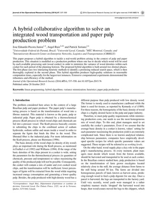
2. feed the cookers. However, the efforts made to increase the
productivity of forestry operations have led to a more efficient,
yet challenging context. The previous practice, where yard
‘desynchronized’ forests and production, has evolved towards
modern yards separated into zones, where each zone is assigned
to a different cooker. In other words, the harvested wood is
transported by a number of fulltruckload trips to the yard zone
corresponding to a specific cooker. This new practice requires
that the plant manager to determine in advance to which yard
zone, and therefore to which cooker, the wood from the
harvested forest will be assigned. It follows that both transpor-
tation and transformation activities are synchronized by the
transportation and production plan. Also, in order to simplify
wood yard operations, this new management model requires
that all the wood coming from the same harvested area be used
before using the one coming from another area. Indeed, this
strategy minimizes both traffic handling at the wood yard and
the amount of wasted wood.
Taking this into account, our industrial partner’s production is
managed in the following way. First, he considers the available
wood within a fixed planning horizon, each period being a
working week. Then, he considers five potential working levels,
each corresponding to a specific basic density. Based on these
inputs, he simultaneously sets the working levels for every cooker
during each planning period and selects the harvested wood to
transport to the factory and its assignment to cookers. This is
done in such a way that, for each cooker and for each period on
the planning horizon (1) the variance of the basic density in a
cooker is minimized and (2) the difference between the average
basic density and the ‘target’ one (ie the one for which the
cooking parameters have been set) is also minimized. Figure 1
summarizes the decisions to be made by plant managers.
This paper contributes a two-phase solution approach to this
difficult problem. In the first phase, two simple heuristics
cooperate to build a restricted search space. This search space
is then explored during the second phase. The remainder of this
paper is organized as follows. The following section positions
this work with respect to previous operations research applica-
tions made in the forestry field. It also reviews some relevant
papers allowing the interested reader to survey hybrid algo-
rithms or hybrid solution approaches. Section 3 will introduce
the two mathematical models used in this work. Section 4 will
describe the overall structure of the proposed hybrid algorithm.
Computational results will be presented and analysed in
Section 5. Finally, Section 6 concludes the paper.
2. Related works in the literature
Since this work presents the development of a new search
algorithm for a very specific industrial context, this section is
divided into two distinct parts. The first part focuses on the pulp
and paper industry. More specifically, it reports some of the
most recent and relevant works regarding operations research
application to solve production planning and transportation
problems in this industry. The second part introduces the reader
to the field of hybrid algorithms, an emergent and promising
approach in the operations research field to solve combinatorial
problems. In both cases, reporting an exhaustive literature
review would be far beyond the scope and the needs of this
work. Nonetheless, the objective of this section is to allow the
reader to position this contribution within the two mentioned
research streams.
In the last years, the number of operations research contribu-
tions made to the forestry supply chain, particularly to the pulp
and paper industry, has rapidly increased. These contributions
deal with a wide range of problems, from long-term strategic
problems related to forest management or company develop-
ment to very short-term operational problems, such as planning
for real-time log/chip transportation or cutting. D’Amours et al
(2008) provide a very interesting review of applications of
operations research techniques, including strategic and tactical
planning as well as operational issues. Strategic planning
focuses mostly on decisions regarding wood availability and
facility design. Growing a forest to maturity is a very slow
process. Although eucalyptus is one of the fastest growing trees
and the sole species exploited by our industrial partner, it still
requires between 5 and 7 years of growth before it can be
harvested. Tactical planning policies and their impact on the
forestry supply chain performance have been studied by Santa-
Eulalia et al (2011). On the other side of the spectrum,
operational planning is concerned with the optimization of
harvested resources and machinery, pulp production planning,
and wood transportation.
Wood transportation activities have received a considerable
amount of the researchers’ attention. Moura and Scaraficci
(2008), using a hybrid GRASP–Linear Programming Meta-
heuristic, scheduled the wood transportation from harvested
areas to mills on a day-to-day basis on a 1-year horizon.
De Lima et al (2011) proposed a log stacking allocation
problem. The authors defined operational issues as the difficulty
to move forestry equipment, the difficulty in log stacking, and
Wood
Forest
Which parcel
should be
harvested? Which harvested
wood should be
assigned to which
cooker?
To elaborate a production plan minimizing the variance of wood
density at each cooker and period.
Which wood
should be used at
each period?
Which parameters
should be elected
for each period?
When should it be
transported to the
mill?
Woodyard Cookers
DecisionsGoal
Figure 1 Decisions related to the integrated wood production and
paper pulp production problem.
538 Journal of the Operational Research Society Vol. 67, No. 4

3. the distance between stacks and existing roadways. They
proposed a solution approach that uses a geographic informa-
tion system to classify potential locations and evaluate opera-
tional issues. They modelled the problem as a linear
programming formulation. The transportation of logs from
forest areas to wood mills has also been addressed as a vehicle
routing problem in El Hachemi et al (2011). The authors used a
hybrid solution approach encompassing constraints program-
ming and linear programming optimization, these methods
being linked by the communication of global constraints. Their
objective is to minimize the cost of the unproductive activities.
Bredström and Rönnqvist (2008) also model a wood transporta-
tion situation as a vehicle routing problem, but in their case,
time windows and synchronization constraints are considered.
Synchronization constraints express the simultaneous availabil-
ity of resources, for example, the availability of a ‘loader’
(a crane that loads the logs on the trucks) at the truck arrival.
The problem described in this work starts at the end of the
forest harvesting planning, as described in Rönnqvist (2003),
but does not account for transportation issues such as those
presented in the above-mentioned works or in Karlsson et al
(2003). In fact, this problem uses the output of the short-term
harvest planning as its input (the available harvested areas
waiting for transportation) and provides the data for transporta-
tion models detailing which week each harvested area should be
transported and to which facility it should be fed. More
precisely, the problem studied here is based on the one
presented in Pécora et al (2007) to which we refer the reader
for a detailed version. In this study, the authors provided a
mathematical model and proposed a constructive heuristic to
solve it. As described in Pécora et al (2007), the efficiency of
exact methods applied to this problem is very limited, mostly
due to the slow convergence of the linear relaxation. To
overcome this obstacle, this paper proposes a new hybrid
heuristic that exploits the decisional structure of the problem.
Hybrid heuristics will be now discussed briefly.
Within the operations research literature, the term ‘hybrid
solution approach’ is generally applied to the combination of
two (or more) different solution methods to promote the
exploration of new search regions, of escaping the local
attraction of optimal points or of generating cuts, among others.
The approach proposed here clearly falls within this rapidly
growing field. However, it can be argued that its fundamental
principle differs from the ones that have until now underlined
the majority of hybrid approaches. As any two solution
methods can be combined to create a hybrid method, the
number of possible hybrid approaches is quite important.
Therefore, the literature on hybrid algorithms is rather large
and fast growing. Nevertheless, some works have attempted to
review and classify this research stream. More notably, several
authors have proposed a taxonomy on hybrids based on the
nature of the methods being hybridized. Talbi (2002) was
among the firsts to provide an extensive classification of hybrid
methods using heuristics while Puchinger and Raidl (2005)
focused on heuristic-exact hybrid methods. Jourdan et al (2009)
proposed a taxonomy on hybrids heuristic-exact methods based
on the work of Talbi (2002). Jourdan et al (2009) classified the
design of each hybrid into high level or low level; the latter
corresponds to the case where a given function of a metaheur-
istic is replaced by another method and the former corresponds
to different algorithms being self-contained. They also classi-
fied hybrid methods in terms of their cooperation mechanisms
into ‘relay’ and ‘teamwork’. ‘Relay’ corresponds to a set of
methods being applied one after the other and each using the
output of the previous as its inputs acting in a pipeline fashion
while ‘teamwork’ represents cooperative optimization models.
More recently, Antonio Parejo et al (2012) proposed a survey
on optimization metaheuristics frameworks and Blum et al
(2011) contributed a survey on hybridization of different
methods of any nature: metaheuristics with metaheuristics,
metaheuristics with constraints programming, metaheuristics
with tree search techniques, metaheuristics with problem
relaxation, and metaheuristics with dynamic programming.
Their paper surveyed 169 works on hybrids and concluded
with a brief guideline to develop hybrid algorithms. It can be
observed that although hybrid approaches have traditionally
merged exact and/or heuristic algorithms (Gallardo et al, 2007),
more and more research is devoted to hybrid methods including
other approaches such as simulation (Peng et al, 2006),
constraint programming (Correa et al, 2004; Hooker, 2006),
neural networks (Pendharkar, 2005; Sahoo and Maity, 2007)
and multi-agent approaches (Yan and Zhou, 2006).
In the particular context of pulp and paper production,
Bredström et al (2004) proposed a hybridization of two mixed
integer models that determined the daily supply chain decisions
of a pulp mill plant over a planning horizon of 3 months. The
first model planned the production for each mill over a 3-month
horizon and solved it using a column generation approach. The
second model used binary variables to represent the explicit
decisions regarding which product to produce on each day.
According to the authors, the solutions generated by their
models are both useful and more effective than the ones
generated manually.
Before moving to the mathematical formulation of the
problem, a word must be said in regard to the maximization of
homogeneity or, in other words, the minimization of a disper-
sion measure, a central issue of the problem at hand. Fisher
(1958) studied maximum homogeneity problems in the context
of partitioning data samples into groups. He divided them into
two classes. The first class dealt with what he calls unrestricted
problems, that is problems where no a priori conditions are
imposed on the observations to be grouped. These problems can
easily be solved by approaches based on sorting and contiguous
partitioning of the sorted observations. The second class deals
with restricted problems, that is problems where conditions are
imposed on the observations to be grouped. In this case, no
simple general solution method is available. The problem
described here falls within the second class. Maximizing the
homogeneity of a partition is, of course, equivalent to minimiz-
ing the sum of the variance of its elements.
Jose Eduardo Pecora et al—A hybrid collaborative algorithm 539

4. 3. Mathematical formulations
This section first presents a mathematical formulation,
which will be referred to as L-problem (for Level Problem),
aimed at answering the questions with which the plant
engineers described in the Introduction are faced. More
precisely, it decides how to: (1) select the wood and
determine its assignment to cookers and (2) select the choice
of working levels for each cooker and period. This is done in
such a way that the difference between the selected target
density and the average basic density of the wood fed at each
cooker and for each period is minimized.
Pécora et al (2007) already faced the problem of minimizing
the deviation of the wood densities within each cooker. In their
paper, they proposed a linearization strategy based on the
definition of a set of discrete density ranges what we, in other
words, call working levels. However, the model proposed in
Pécora et al (2007) had to be adapted to cope with the new
wood yard practices. In particular, since forest parcels produce
similar volumes of wood that need to be completely consumed
by a given cooker before starting with another parcel, our new
model does not take into account forest volumes, nor inventory
constraints. Despite these simplifications, the formulation pro-
posed for the L-problem remains very difficult to solve in real
sized instances as the ones found in the industry.
We also define a second problem namely the V-problem (for
Variance-problem), which aims at scheduling and assigning the
available wood among cookers in such a way that the variance
of the basic density for each cooker and period is minimized.
One could think that the V-problem is better suited to the real
plant managers’ problem than L-problem since it directly
minimizes the density variance within each cooker. However,
solutions to the V-problem, although very appealing with
respect to their density variance, may lead to average density
values for which the company does not have an optimized
receipt. Nevertheless, the V-problem is far from useless as it
may, in fact, contribute crucial information on how to form
good (ie low variance) wood arrangements. This information
will be used in the algorithmic scheme presented in Section 4,
which will help us solve the L-problem. However, before
getting into the hybrid solution approach, let us first introduce
some basic notation and present both models.
Let T be the planning horizon, where each period t is 1 week
long, and W be the set of harvested areas waiting for transporta-
tion. Note that harvest areas are not all available for transporta-
tion at the same time: some forests are very young, some are
very old, and others are not dry enough for pulp production
purposes. Thus, each harvest area w ∈ W is associated with a
transportation window identified by τwt, which takes value 1
when the harvest area w is available for transportation at period
t and zero otherwise. Finally, each harvest area w is also
characterized by the average basic density δw of the wood from
that area.
On the manufacturing side, we consider a single plant having
several pulp processing units identified by index f ∈ F. Let L be
the set of predefined working levels used in the plant. The
parameters for each level l have been adjusted for a specific
wood density, that we will call the target density and denote by
δl. The pulp demand for every cooker and period, denoted by
dft, is deterministic. It is assumed to be less than the correspond-
ing cooker production capacity and is given as a number of
harvest areas. The volume of available wood in each harvest
area is not explicitly considered in the demand satisfaction
constraints because, in the particular context modelled here, all
harvest areas are planted specifically for pulp manufacturing
purposes and their volumes are basically the same. Thus, one
can easily simplify these constraints by considering the
demands as a fixed number of harvest areas without much loss
of precision.
Let us also introduce decision variables xwft, which take value
1 when the harvest area w is processed by cooker f at period t,
and zero otherwise, and decision variables yftl, which take value
1 if the cooker f is set at production level l during period t and
zero otherwise. Two sets of real and positive auxiliary variables
are also required: σftl, which is used to compute the deviation
between the basic densities of the wood assigned to a given
cooker and the target basic density that has been selected for the
cooker, and sftl, which act as explicit slack variables. L-problem
is therefore formulated as follows:
L-problem
Minimize ZL
=
X
t
X
f
X
l
σftl (1)
Subject to :
X
l
yftl = 1 8f ; t ; (2)
sftl ⩽ M 1 - yftl
À Á
8f ; l; t ; (3)
X
w
δw - δlð Þ2
xwft = σftl + sftl 8f ; l; t ; (4)
X
f
xwft ⩽ τwt 8 w; t ; (5)
X
f
X
t
xwft ⩽ 1 8w ; (6)
X
f
Xt0
t = 1
xwft = 1 8 w 2 Wt0 ; 8t0
2 T ; (7)
X
w
xwft = dft 8 f ; t ; (8)
xwft; yftl 2 B 8 w; f ; t; l ; (9)
σftl; sftl 2 R+
8f ; t; l ; (10)
L-problem aims at minimizing the sum over all the cookers and
periods of the difference between the target density and the
average density of the wood assigned to each cooker, which is
540 Journal of the Operational Research Society Vol. 67, No. 4

5. computed by variables σftl. To this end, constraints (2), (3) and
(4) are required. Constraints (2) state that one and only one
density level per digester and period will be chosen (ie the target
level). Then, note that constraints (3) allow variables sftl to take
any positive value bounded by M when digester f is not planned
to operate at level l in period t. However, sftl are forced to zero
for the selected target densities. Constraints (4) compute the
wood densities’ deviation within each digester with respect to
the target level, putting the result either in σftl—for the selected
digester target level—or in sftl—for the other working levels.
Constraints (5) state that each harvest area can only be used
within its time window while constraints (6) ensure that the
same harvest area cannot be used more than once. In the real-
life application modelled here, certain harvest areas are required
to be used before the end of the current planning horizon,
generally because they have been harvested for some time
already and must be transported and processed before they
become unfit for processing. Set Wt′⊂W identifies such forest
units and constraints (7) force the model to use all such harvest
areas (ie those that must be used before the end of the period t′).
Demand satisfaction is ensured through constraints (8). Finally,
constraints (9) and (10) define the variable ranges.
The L-problem is related to the generalized assignment
problem, which has been to be NP-hard (Martello and Toth
(1990)). Solving it is, therefore, a very difficult task mainly
because its relaxation results in very poor lower-bounds. In fact,
constraints (3) are useful only when the variables are integer. In
consequence the linear relaxation adjusts itself to get a null
objective function, so the algorithm executes too many itera-
tions to increase the lower bound. Therefore, real-world
instances cannot be solved in reasonable time and a heuristic
approach seems adequate to tackle the L-problem efficiently.
To this end, we realized that despite the target levels, plant
engineers try to group available wood so that they may reach
the highest homogeneity in each cooker and each period.
Following this idea, we formulated the V-problem (for Var-
iance-problem). V-problem aims at assigning the available
wood among cookers in such a way that the variance of
the basic density for each cooker and period is minimized.
The V-problem is subjected to the same practical constraints as
the L-problem (demand satisfaction, use of the woods within
the given time windows) but it does not take into account the
choice of settings for the cookers (ie the target densities). Using
the notation introduced previously, the V-problem can be
formulated as the following integer non-linear model.
V-problem
Minimize ZV
=
X
w
X
t
X
f
δw -^δft
À Á2
xwft (11)
Subject to :
P
w
δwxwft
P
w
xwft
=^δft 8 f ; t ; (12)
X
f
xwft ⩽ τwt 8 w; t ; (13)
X
f
X
t
xwft ⩽ 1 8w ; (14)
X
f
Xt0
t = 1
xwft = 1 8 w 2 Wt0 ; 8t0
2 T ; (15)
X
w
xwft = dft 8 f ; t ; (16)
xwft 2 B ; ^δft 2 R+
(17)
The objective function (11) is the sum of the squared difference
between the basic density of the allocated wood and the average
working density for each cooker and period. In other words,
(11) minimizes the dispersion of the wood density. Precisely,
the average basic density for each cooker at each period ^δft is
computed by constraints (12). Constraints (13) – (16) are, of
course, the same as defined in L-problem. Finally, we find
constraints (17) on the nature of the variables used in the model.
The previous paragraphs presented two similar, yet different
problems, and their respective formulations. These problems
present complementary perspectives to the situation faced by
the plant engineers. Indeed, solving the V-problem is quite
appealing because it will minimize the overall density variance
of the wood processed by each cooker. However, it does not
account for the density’s proximity, or distance, to one of the
discrete levels corresponding to the prefixed factory settings.
On the other hand, the L-problem minimizes the variance of the
wood assigned to each cooker and period with respect to the
elected target density, but solving it is far beyond the ability of
commercial branch-and-bound solvers.
In order to solve the problem faced by plant engineers, the
next section proposes a two-stage hybrid approach that com-
bines the information obtained by the two proposed models.
To this end, we will denote δV
ft =^δft as the average density of the
wood assigned to each cooker and period, and δft
L
as the target
basic density elected for each cooker and period. The compar-
ison between δft
V
and δft
L
will be used to identify promising
search directions during the execution of the heuristic algo-
rithm, as will be explained in the next section.
4. The search algorithm
The main idea of the proposed search algorithm is to reduce the
size of the potential solution space in order to concentrate the
search to a specific sub-region, which could be explored to
optimality in an efficient manner.
The search algorithm is comprised of two phases: the space
restriction phase and the search phase. The space restriction
phase aims to identify sub-regions of the solution space, which
offer a high potential for near optimal, if not optimal, solutions.
Once this process has been completed, the resulting Restricted
Jose Eduardo Pecora et al—A hybrid collaborative algorithm 541

6. Space (RS) is thoroughly explored by either an exact method or
a dedicated local search algorithm. When applied to the
problem considered here, and during the space restriction phase,
subsets of potential working levels for each cooker and period
are elected to form a sub-region of the solution space. These
subsets will then be used as constraints during the search phase
of the L-problem formulation, which will hopefully be solved to
optimality. The next section focuses on the hybrid approach that
we propose for building the RS.
4.1. The restriction phase
The objective of the restriction phase is not to find an
optimal solution but to identify a promising sub-region of
the solution space. This will be achieved by means of an
iterative approach in which, at each iteration, a region of the
solution space is probed. Probing a region consists in
generating a solution that may give us an idea of the region’s
potential for containing high quality solutions. After few
iterations, the algorithm examines the structure of the
solutions produced and builds a restriction, the RS, on which
a thorough search will be executed during the search phase.
The question now is how to probe the solution space. If you
recall, Section 3 proposed formulations for the L-problem
and the V-problem. Both formulations are difficult to solve
(note that V-problem has a non-linear objective function), so
we propose two simple but efficient heuristics (namely
L-heuristic and V-heuristic) to produce solutions to these
problems.
L-heuristic decomposes the whole problem into |T| individual
periods that can be solved sequentially, from period t = 1 to
period t = T, using the formulation provided in Section 3.
V-heuristic is a construction algorithm that allocates one by
one the available forests to cookers in order to minimize the
variance of the wood allocated to each digester and period.
After allocating all the wood, a 2-OPT neighbourhood local
search tries to exchange the allocation of pairs of forests in an
attempt to reduce the total density variance. Both L-heuristic
and V-heuristic are presented in the Appendix section. Also, an
information exchange mechanism has been designed in order to
guide the search performed by these heuristics. This whole
process is illustrated in Figure 2.
The restriction space building process consists of the follow-
ing four steps.
1. The process starts by calling the L-heuristic on the whole
solution space. L-heuristic (see Appendix section ‘The
constructive L-heuristic’) produces a feasible solution to
the L-problem, which specifies a unique working level for
each cooker and period by means of variables yftl, which are
related to unique density values δft
L
.
2. The set of target densities produced by the L-heuristic are
then passed to the V-heuristic (see Appendix section
‘A location heuristic to solve the V-problem’), which uses
these values as the ‘reference’ density or, in other words, the
average density with respect to the variance to be minimized
for each cooker and period. Executing the V-heuristic,
therefore, produces a feasible solution that assigns available
wood to cookers in order to minimize the variance with
respect to the target density. The wood assignments pro-
duced by the V-heuristic allow to compute δft
V
, the average
wood density for each cooker and period.
3. At this point, it is possible to compute Δft = δft
V
− δft
L
, which
evaluates the gap between the ‘elected’ density for each
cooker and period, δft
L
and the average density reached by the
wood assignment proposed by the V-heuristic, δft
V
. We will
refer to Δft as direction vectors. Direction vectors are
computed for every cooker and period in order to drive the
search towards more promising solutions. These new search
directions, which take the form of restrictions on the yftl
variables, are added to the L-problem. The constraints added
in previous iterations are then deleted, and the algorithm
moves to step 1 to perform a new iteration. At each iteration,
new restrictions are applied, limiting the feasible solution
space. The algorithm stops the restriction phase after a
prefixed number of iterations or as soon as the size of the
incumbent solution space is large enough.
4. After a given number of iterations and once the solution space
has been probed adequately, an RS is built by looking at the
solutions produced by the L-heuristic and V-heuristic during
the restriction phase. The RS is then explored thoroughly by
means of an exact, or a dedicated search method.
The following paragraphs describe the way in which informa-
tion is extracted from the analysis of the direction vectors and
how this information is introduced into the following iterations.
We also explain how the RS is built to complete the
restriction phase.
Direction vectors. Direction vectors allow us to evaluate if
homogeneous groups of wood can be formed for specific fac-
tory working levels. A zero, or a rather small, direction vector
is consistent with a good wood assignment, that is a wood
assignment with a small variance with respect to the elected
working level for the cooker f at period t. On the other hand, if
the results obtained from the methods differ greatly, it implies
that forming homogeneous density assignments around the
level chosen will be difficult and, therefore, that the level
should be reconsidered.
Whenever the two methods do not agree on the value that the
working density should take, Δft can be viewed as a suggested
search direction. To better illustrate this notion, let us introduce
Figure 3 that shows direction vectors Δ1 – Δ5 obtained for each
of the planning periods t = 1, …, 5 for a given cooker.
Figure 3 presents the prefixed density working levels (L1 – L5)
corresponding to unique yftl. It also shows three types of direction
vectors. The first type corresponds to the case illustrated
by vectors Δ1 and Δ2. The second type corresponds to direction
vectors Δ3 and Δ4. The last type is illustrated by direction
vector Δ5. Each case is explained in the following paragraphs.
542 Journal of the Operational Research Society Vol. 67, No. 4

7. Direction vectors Δ1 and Δ2 point to, respectively, higher and
lower density than the ones elected for the cooker. In particular,
since Δ1 indicates that the average density of the wood assign-
ment is much higher than the density level elected for the
cooker, we conclude that the current density level and those
below (ie L1) do not seem adequate and, in consequence, will
not be considered in the forthcoming iterations. To this end, a
constraint like:
X
ðftlÞ2G0
1
yftl = 0 (18)
will be added to L-problem at the following iteration. In this
equation, G′1 is the set of levels l, which should be
forbidden for a given cooker and period. In a similar
manner, Δ2 allows us to postulate that the current level plus
those higher than L4 seem rather inappropriate and they can
be forbidden in further iterations.
Direction vectors Δ3 and Δ4 point to densities out of the valid
density range. We conclude that the current levels are the most
promising and that these levels will, therefore, be fixed
for the next iteration. This can be done by adding a constraint
similar to Equation (18) to the L-problem and extending it to a
different set G′1 of variables. For example, if we consider
Δ3 in Figure 3, the following equation should be added:
y(1, 3, 1) + y(1, 3, 2) + y(1, 3, 3) + y(1 ,3, 4) = 0.
The last type of direction vector is illustrated by Δ5 and it
corresponds to the situation where both the L-heuristic and
the V-heuristic agree on the target and elected densities.
In this case, we can conclude that choosing the elected
level was a good decision and that this level will, therefore,
be fixed for the next iteration. In the particular case
shown in Figure 3, the following constraint will be used:
y(1, 5, 1) + y(1, 5, 2) + y(1, 5, 3) + y(1, 5, 5) = 0.
It can also be observed that, while the last two types of
direction vectors tend to concentrate the search in the same
region of the solution space by fixing variables at their current
values, the first type of direction vector forces the search to
other non-explored regions, forming a kind of intensification/
diversification mechanism.
Figure 2 The hybrid algorithm.
Figure 3 Example of direction vectors.
Jose Eduardo Pecora et al—A hybrid collaborative algorithm 543

8. Building the RS. In order to define the RS, we keep track of
the different solutions produced by the L-heuristic and the
V-heuristic during the restriction phase and use them to build
an ‘envelope’ on the density variables. Let S be the set for the
density variables δft
i
, associated with the solutions found in the
restriction phase. These solutions are indeed local optima for
their respective models. If the number of cycles in the restric-
tion phase is N, then |S| = 2N represents half of the solutions
coming from each heuristic method. Among the different
ways of defining a restriction to the original search space
based on the information gathered by the L-heuristic and
V-heuristic, we propose to constrain the range of values for
density variables by δft⩽δft⩽δft, where δft and δft are, respec-
tively, the lowest and the highest values found for variable δft
during the restriction phase. Bounding the average basic den-
sity in the L-Model is the equivalent of forcing the levels out-
side these bounds to be zero. This can be done by adding
constraints similar to (18). The chosen region will encapsulate
the density variables inside a convex envelope, making the
search space smaller than the original one. Since all the visited
local optimal solutions are inside the envelope, this region is
guaranteed to contain feasible solutions.
4.2. Search phase
The search phase performs a thorough search on the RS. In
our case, we solved the L-Model presented in Section 3 to
optimality within the bounds given by the RS. To this end, a
commercial branch-and-bound solver (Cplex 12.5.1.0)
was used.
Obviously, the restriction phase plays a key role in the
algorithm, and a careful choice of the RS’s size is needed in
order to reach a satisfactory efficiency. If the restriction phase
produces a very narrow RS, then the RS may be thoroughly
explored with a reasonable computational effort, which is an
excellent thing. However, a very narrow RS also increases the
chances of missing high-quality solutions. While a wide RS
improves the likelihood for high quality solutions it becomes
difficult to explore efficiently and, even if it contains very good
solutions, one risks missing some of them. Discussion on this
important issue is provided in the next section and presents the
numerical experiments.
5. Computational experiments
This section is divided into two main parts; the first is aimed at
explaining the different trade-offs underlying the parameters’
setting process. The second part seeks to assess the potential of
the proposed approach by comparing the quality of the
solutions obtained to the one produced by its component
methods and a commercial branch-and-bound software.
Our test bed contains 100 instances inspired by real data
provided by a Brazilian company. The industrial setting
considered has three identical cookers. Plant managers elected
five working levels (l1 – l5). Instances are divided into three
groups according to the number of periods covered by the
planning horizon T = {16, 32, 52}. Test instances also differ in
the number of available forests to allocate W = {400, 600, 800,-
1000}. Finally, to increase the robustness of our tests, we
generated a forest basic density by drawing from a normal
distribution where the average is 530 and standard deviation
D = {50, 100}. Groups T = 52 (which represents the planning
for 1 year) and T = 32 have 40 instances each, while the group
T = 16 contains 20 instances, as described in Table 1. All tests
were performed on Intel(R) Xeon(R) X5675 @ 3.07GHz
computer with a Linux operating system.
5.1. Parameters setting
One of the greatest challenges of the approach presented in this
paper lies in determining the RS’s size. To formalize things, let
us define the RS’s size as the quantity of free yftl variables
in the RS or, in other words, variables that have not been forced
to a value. Undeniably, the larger the RS, the greater the
chances of it yielding good solutions or even the optimal
solution. On the other hand, the larger the RS, the harder it is
to explore thoroughly. Several preliminary experiments were
conducted in order to empirically estimate an efficient trade-off
between the size of the RS and the computational time required
to explore it. More precisely, we intended to estimate the
empirical relationship between the RS’s size and the time
required by the branch-and-bound software to explore it to
optimality. Our experiments showed that most of the RSs with
30 or less free variables were solved to optimality in less than
1 h. Since, for us, 1 h qualified as a reasonable amount of
computational effort to solve a problem like the one presented
here, we arbitrarily decided to aim for RS with approximately
20–30 free variables. Consequently, the number of free vari-
ables is counted after each iteration of the restriction phase and,
if it is greater than 20, then the algorithm generates the RS and
proceeds to the Search phase. If there are less than 20 free
variables, then a new iteration of the restriction phase is
executed.
Finally, three different types of direction vectors were
presented in Section 4, but nothing was said about how many
of them, if not all, should be used at each iteration. Using too
many direction vectors should constrain the RS very quickly
and, therefore, limit the information exchange between the
L-heuristic and the V-heuristic. However, if the information
contained in the direction vectors is not used, then the search
is not guided, and the expected synergy between the heuris-
tics simply disappears. After preliminary experiments, we
Table 1 Description of the testbed
T 16 16 32 32 32 32 52 52 52 52
W 400 400 400 400 600 600 800 800 1000 1000
D 50 100 50 100 50 100 50 100 50 100
# instances 10 10 10 10 10 10 10 10 10 10
544 Journal of the Operational Research Society Vol. 67, No. 4

9. established two rules in order to ensure that the restriction phase
executed at least two iterations before producing an RS of the
desired size. First, we decided to implement all the direction
vectors of types two and three. If a direction vector was under
10% of the density difference between two levels, it was
classified as a type 3. The second rule concerns the selection
and the number of direction vectors of type 1 to use. In this
case, we elected to use 10% of the direction vectors of type 1
having the largest module. Our preliminary experiments
revealed that, although these rules did not produce the best
results for all the cases, they were proven to be the most robust.
5.2. Performance tests
This section aims at assessing the performance of the proposed
solution approach in terms of both the quality of the solutions
produced and the computational time required to achieve them.
To this end, each instance in the test bed was solved by the
collaborative RS heuristic where the computational time
allotted to the search phase was limited to 1 h. Since the
RS production required less than 100 s in every case, it
seemed fair to us to say that the RS heuristic was allotted 1 h
of computational time. We also solved the L-Model for-
mulation for each of the instances proposed using the
commercial solver Cplex 12.5.1.0. We recorded the best
integer solution produced by Cplex after 1 h and 10 h of
execution, respectively. It is important to mention that,
even after 10 h of computing, Cplex was not able to close
the optimality gap. More specifically, in the best cases and
after 10 h of computing time, Cplex was able to close to 87%
the optimality gap produced for instance 32-400-100-10.
Optimality gaps for all the others instances were well
above 90%. Consequently, in the sequel we will discuss
the performance of the proposed solution methods with
respect to the results produced by the RS heuristic rather
than to lower bounds. We will also report the best
solutions produced by both the L-heuristic and the V-
heuristic during the restriction phase. In the case of the
solutions produced by the V-heuristic, the chosen levels
correspond to the ones closest to the average density for
each cooker and period. This comparison will allow us to
analyse the added value of the information exchanged
between the two methods.
The computational results are presented in Tables 2–4.
In these tables, the first four columns give the characteristics of
the instances. The four following columns report the gap
between the solution produced by each of the considered
methods and the RS-heuristic solution. The gap is computed
using the equation:
Gap =
ZMethod - ZRS
ZRS
100 % (19)
where ZRS is the objective function returned by the RS-heuristic
and ZMethod is the value given by each of the other considered
solving methods, respectively, L-heuristic, V-heuristic, Cplex
1 h and Cplex 10 h.
Table 2 Computational results for T = 16 periods
T W D I L-heuristic (%) V-heuristic (%) Cplex 1 h (%) Cplex 10 h (%)
16 400 100 1 12.37 36.95 2.42 − 0.78
16 400 100 2 23.83 57.03 3.11 − 0.74
16 400 100 3 28.73 47.55 3.67 − 0.18
16 400 100 4 19.06 35.14 0.14 − 0.90
16 400 100 5 30.53 27.25 3.62 − 1.95
16 400 100 6 20.34 58.15 − 1.77 − 5.90
16 400 100 7 37.01 49.31 3.13 − 2.63
16 400 100 8 41.92 43.84 3.71 0.45
16 400 100 9 37.55 45.96 5.71 − 1.16
16 400 100 10 15.20 39.98 5.42 0.24
Average 26.66 44.12 2.92 − 1.35
16 400 050 1 7.15 32.59 0.95 − 0.15
16 400 050 2 7.31 25.76 0.47 − 0.87
16 400 050 3 6.87 37.38 − 0.14 − 0.15
16 400 050 4 10.77 56.02 − 1.66 − 1.77
16 400 050 5 7.47 39.13 2.17 0
16 400 050 6 13.28 40.18 0.24 − 0.44
16 400 050 7 3.80 22.88 1.17 0
16 400 050 8 8.71 32.75 1.85 − 0.07
16 400 050 9 19.46 30.05 0.86 0
16 400 050 10 3.79 30.81 − 0.56 − 3.02
Average 8.86 34.75 0.53 − 0.65
Average over 20 instances 17.76 39.43 1.72 − 1.00
Number times RS is better 20 20 16 6
Jose Eduardo Pecora et al—A hybrid collaborative algorithm 545

10. Table 2 reports the results produced for instances contain-
ing T = 16 periods. As one could expect, both the L-heuristic
and V-heuristic produced very poor results, with average
gaps of 17.76 and 39.43%, respectively. When comparing
the results produced by Cplex, it can be observed that the RS-
heuristic improves the Cplex 1 h results in 16 out of 20 cases
and those produced by Cplex after 10 h of computing in 6 out
of 20 instances. More precisely, the RS-heuristic results are
on average 1.72% better than those produced by Cplex after
1 h, but 1% worse than the ones produced by Cplex after
10 h. In general, and for these very small-sized instances,
Cplex is very efficient but the RS-heuristic performs also
very well. It is worth mentioning that it appeared more
difficult to solve instances where the forest’s basic density
was generated with a larger variance (D = 100). In fact, the
average gaps obtained for these instances were larger than
Table 3 Computational results for T = 32 periods
T W D I L-heuristic (%) V-heuristic (%) Cplex 1 h (%) Cplex 10 h (%)
32 600 100 1 20.86 32.18 16.00 1.44
32 600 100 2 17.48 60.46 6.12 0.33
32 600 100 3 25.60 21.08 4.61 − 1.41
32 600 100 4 22.74 27.30 2.65 − 0.45
32 600 100 5 15.61 36.75 7.38 0.61
32 600 100 6 28.08 30.19 18.46 − 0.49
32 600 100 7 20.38 23.71 7.12 0.48
32 600 100 8 11.53 46.53 12.28 − 0.25
32 600 100 9 17.21 33.57 8.33 4.02
32 600 100 10 53.54 32.06 7.78 0.09
Average 23.3 34.38 9.07 0.44
32 600 050 1 8.99 4.13 1.14 − 1.37
32 600 050 2 10.15 16.89 2.36 0.19
32 600 050 3 8.22 15.81 13.00 3.36
32 600 050 4 4.96 19.78 4.95 − 0.20
32 600 050 5 8.97 28.13 5.22 0.19
32 600 050 6 11.97 25.08 0.49 0.27
32 600 050 7 11.18 11.50 − 0.07 − 5.04
32 600 050 8 13.15 22.27 − 0.67 − 1.28
32 600 050 9 5.27 32.78 4.27 − 0.35
32 600 050 10 8.22 15.81 13.00 0.09
Average 9.11 19.22 4.37 − 0.41
32 400 100 1 15.9 36.90 10.95 − 0.28
32 400 100 2 24.60 39.61 19.28 − 1.34
32 400 100 3 24.07 27.37 0.53 − 1.25
32 400 100 4 17.32 71.34 12.11 − 2.81
32 400 100 5 34.63 31.97 2.89 − 1.81
32 400 100 6 19.90 44.42 6.61 0.09
32 400 100 7 17.70 34.81 13.22 0.91
32 400 100 8 45.44 48.56 1.54 − 0.94
32 400 100 9 23.81 60.15 0.27 − 3.48
32 400 100 10 16.46 24.61 1.23 − 2.37
Average 23.98 41.97 6.86 − 1.33
32 400 050 1 5.35 20.26 1.48 0.19
32 400 050 2 21.89 22.57 11.15 0
32 400 050 3 10.34 24.83 9.07 0
32 400 050 4 11.62 17.00 0.83 − 0.85
32 400 050 5 9.65 24.54 6.68 0.12
32 400 050 6 5.71 22.53 3.30 − 0.65
32 400 050 7 17.25 12.13 2.82 − 0.61
32 400 050 8 10.92 21.22 3.48 0
32 400 050 9 14.17 27.31 3.18 − 0.34
32 400 050 10 9.10 16.34 5.12 0.18
Average 11.6 20.87 4.71 − 0.20
Average over 40 instances 17.00 29.11 6.25 − 0.38
Number times RS is better 40 40 38 14
546 Journal of the Operational Research Society Vol. 67, No. 4

11. those obtained when (D = 50), whichever the method
considered.
Table 3 reports the results produced for instances containing
T = 32 periods. For these mid-sized instances, the RS-heuristic
performs much better than Cplex 1 h but slightly worse than
Cplex 10 h. In fact, within the same computing time, the RS-
heuristic improved the results produced by Cplex 1 h in 38 out
of 40 instances and produced better results than Cplex 10 h in
14 of of the 40 instances. For the ‘easy’ instances set (D = 50),
the average gaps produced by Cplex in 1 h range from 4.37 to
4.71% and those produced within a 10-h timespan range from
− 0.41 to − 0.20%. The performance of the RS-heuristic is
therefore very close to the one offered by Cplex 10 h, but
requires only a fraction of the computing time. When consider-
ing the ‘hard’ instances (D = 100), the RS-heuristic beats all the
Cplex 1 h results by 9.07 and 6.86% on average.
Table 4 Computational results for T = 52 periods
T W D I L-heuristic (%) V-heuristic (%) Cplex 1 h (%) Cplex 10 h (%)
52 1000 100 1 49.2% 30.28 9.81 − 2.31
52 1000 100 2 42.37 21.94 8.67 0.81
52 1000 100 3 60.72 31.51 44.64 0.07
52 1000 100 4 41.60 15.23 33.16 − 0.32
52 1000 100 5 45.73 33.43 15.59 − 0.78
52 1000 100 6 46.17 19.10 16.07 − 1.38
52 1000 100 7 51.01 26.31 2.92 − 2.47
52 1000 100 8 43.81 26.08 9.17 − 0.06
52 1000 100 9 60.03 23.44 19.92 5.99
52 1000 100 10 55.26 22.05 34.04 0.05
Average 49.59 24.94 19.4 − 0.04
52 100 050 1 15.99 16.18 4.63 0.8
52 100 050 2 18.20 24.42 36.62 0.21
52 100 050 3 25.39 17.68 8.45 0.71
52 100 050 4 28.18 17.51 4.83 1.09
52 100 050 5 20.51 16.84 9.91 1.35
52 100 050 6 24.36 13.29 0.76 − 0.43
52 100 050 7 25.50 19.29 7.86 0.95
52 100 050 8 21.41 17.44 5.61 − 0.20
52 100 050 9 31.24 24.75 3.04 − 1.24
52 100 050 10 18.56 25.86 17.66 4.09
Average 22.93 19.33 9.94 0.73
52 800 100 1 25.45 27.14 14.22 2.49
52 800 100 2 20.31 28.35 6.34 2.15
52 800 100 3 32.15 38.69 8.26 2.17
52 800 100 4 16.94 27.66 9.30 0.73
52 800 100 5 24.29 56.43 4.23 − 0.05
52 800 100 6 12.25 26.57 6.43 0.17
52 800 100 7 17.77 38.39 14.43 0.75
52 800 100 8 19.89 21.70 7.37 − 0.40
52 800 100 9 21.65 27.76 7.54 1.10
52 800 100 10 25.85 20.26 6.78 − 0.78
Average 21.65 31.29 8.49 0.83
52 800 050 1 14.59 11.27 5.00 0.98
52 800 050 2 11.22 26.83 2.12 − 1.16
52 800 050 3 9.88 19.32 7.93 1.04
52 800 050 4 7.37 24.88 1.66 0.35
52 800 050 5 8.48 18.39 12.83 − 0.17
52 800 050 6 6.41 12.60 0.41 0.11
52 800 050 7 8.48 20.39 3.77 0.06
52 800 050 8 11.8 19.88 2.20 − 0.06
52 800 050 9 7.99 14.28 6.71 3.66
52 800 050 10 12.4 21.72 6.84 − 2.59
Average 9.86 18.96 4.95 0.22
Average over 40 instances 26.01 23.63 10.69 0.44
Number times RS is better 40 40 40 23
Jose Eduardo Pecora et al—A hybrid collaborative algorithm 547

12. Table 4 reports the results produced by the largest-sized
instances containing T = 52 periods. For these instances, the
results produced by Cplex 1 h are clearly outperformed
by the RS-heuristic. In fact, the RS-heuristic produced
better results for all of the 40 instances, improving the
Cplex 1 h results by up to 44.64%, and by more than 10%
on average. When compared to Cplex 10 h, RS-heuristic
produced very similar results. The RS-heuristic improved
Cplex 10 h results in 23 of the 40 instances, with an average
gap of 0.44%.
To summarize, the computational results show that the
two methods used during the space restriction phase, namely
the L-heuristic and the V-heuristic, performed very poorly
when used alone. However, used within the information
exchange scheme proposed here, they contributed to the
definition of a very interesting sub-region in the solution
space. Consequently, search within this restricted region
was more efficient as reported by our extensive numerical
results. In fact, the results produced by the RS-heuristic are
comparable to those produced by Cplex, but they required,
roughly, 1/10 of the computing time.
6. Conclusion
In this work, we proposed a hybrid heuristic method to tackle a
real-world problem arising in the context of pulp and paper
production. This situation is modelled as a production problem
where one has to decide which wood goes to each available
processing unit (wood cooker) in order to minimize the variance
of wood densities within each cooker for each period of
the planning horizon. The proposed solution method is divided
into two phases. In the first phase, two heuristic methods
interact to exchange information on the searched space and
visited solutions in order to find a suitable RS. The second
phase then explores the RS by means of an exact algorithm.
Extensive computational tests proved the efficiency of the RS
heuristic when compared to a standard branch-and-bound soft-
ware and to the results produced by each of the heuristic
methods used in the first phase of the RS heuristic.
Despite the good results produced by the proposed algorithm,
we realized that, in order to increase the method robustness and,
therefore, reduce the possibility of missing high-quality solu-
tions, the size of the RS needs to be kept relatively large. A
natural extension of this study would be to generate several
smaller RS instead of a single one. Doing so, each RS could be
explored more efficiently, and the risk of missing good
solutions would be minimized. We also intend to apply the RS
principles to our future researches and other difficult operations
research problems.
Acknowledgements—This research was partially supported by grants [OPG
0293307 and OPG 0177174] from the Canadian Natural Sciences and
Engineering Research Council (NSERC) and grant [2671/04-2] from
Coordenação de Aperfeiçoamento de Pessoal de Nível Superior (CAPES)
—Brazil. Their support is gratefully acknowledged.
References
Antonio Parejo J, Ruiz-Cortes A, Lozano S and Fernandez P (2012).
Metaheuristic optimization frameworks: A survey and benchmarking.
Soft Computing 16(3, SI): 527–561.
Biermann CJ (1996). Handbook of Pulping and Papermaking. 2nd edn
Academic Press: San Diego, CA.
Blum C, Puchinger J, Raidl GR and Roli A (2011). Hybrid metaheuristics
in combinatorial optimization: A survey. Applied Soft Computing
11(6): 4135–4151.
Bredström D, Lundgren JT, Rönnqvist M, Carlsson D and Mason A
(2004). Supply chain optimization in the pulp mill industry—IP
models, column generation and novel constraint branches. European
Journal of Operational Research 156(1): 2–22.
Bredström D and Rönnqvist M (2008). Combined vehicle routing and
scheduling with temporal precedence and synchronization constraints.
European Journal of Operational Research 191(1): 19–31.
Correa AI, Langevin A and Rousseau LM (2004). Dispatching and
conflict-free routing of automated guided vehicles: A hybrid approach
combining constraint programming and mixed integer programming.
In: van Hentenryck P and Milano M (eds). Integration of AI and OR
Techniques in Constraint Programming for Combinatorial Optimiza-
tion Problems. Lecture Notes in Computer Science, Vol. 3011.
Springer-Verlag Berlin: Berlin, pp 370–379.
D’Amours S, Rönnqvist M and Weintraub A (2008). Using operational
research for supply chain planning in the forest products industry.
INFOR 46(4, Part 2, SI): 265–281.
De Lima MP et al (2011). Methodology for planning log stacking using
geotechnology and operations research. CERNE 17(3): 309–319.
El Hachemi N, Gendreau M and Rousseau L-M (2011). A hybrid
constraint programming approach to the log-truck scheduling pro-
blem. Annals of Operations Research, 184(1):163–178. 5th Interna-
tional Conference on Integration of AI and OR Techniques in
Constraint Programming for Combinatorial Optimization Problems,
Paris, France, 20–23 May 2008.
Fisher WD (1958). On grouping for maximum homogeneity. Journal of
American Statistical Association 53(284): 789–798.
Foelkel CEB, Mora E and Menochelli S (1992). Densidade básica: sua
verdadeira utilidade como índice de qualidade da madeira de eucalipto
para produção de celulose. O Papel 53(5): 35–40.
Gallardo J, Cotta C and Fernandez A (2007). On the hybridization of memetic
algorithms with branch-and-bound techniques. IEEE Transactions On
Systems Man and Cybernetics Part B—Cybernetics 37(1): 77–83.
Hooker JN (2006). An integrated method for planning and scheduling to
minimize tardiness. Constraints 11(2–3): 139–157.
Jourdan L, Basseur M and Talbi EG (2009). Hybridizing exact methods
and metaheuristics: A taxonomy. European Journal of Operational
Research 199(3): 620–629.
Karlsson J, Ronnqvist M and Bergstrom J (2003). Short-term harvest
planning including scheduling of harvest crews. International Trans-
actions in Operational Research 10(5): 413–431.
Kennedy JF, Philips G and Williams P (eds) (1989). Wood Processing
and Utilization. Ellis Horwood Limited: Chichester, West Sussex, UK.
Martello S and Toth P (1990). Knapsack Problems: Algorithms and
Computer Implementations. John Wiley & Sons: New York.
Moura AV and Scaraficci RA (2008). Hybrid heuristic strategies for
planning and scheduling forest harvest and transportation activities. In
Proceedings of 11th IEEE International Conference on Computa-
tional Science and Engineering, São Paulo, Brazil, 16–18 July 2008,
pp 447–454.
Pécora JE, Ruiz A and Soriano P (2007). Minimization of the wood
density variation in pulp and paper production. INFOR 45(4): 187–196.
Pendharkar PC (2005). Hybrid approaches for classification under
information acquisition cost constraint. Decision Support Systems
41(1): 228–241.
548 Journal of the Operational Research Society Vol. 67, No. 4

13. Peng J, Shang G and Liu H (2006). A hybrid intelligent algorithm for
vehicle routing models with fuzzy travel times. In: Computational
Intelligence: International Conference on Intelligent Computing,
ICIC 2006, Kunming, China, August 16–19, 2006, Lecture Notes in
Computer Science, Springer, Berlin Heidelberg.
Puchinger J and Raidl GR (2005). Combining metaheuristics and exact
algorithms in combinatorial optimization: A survey and classification.
In Artificial Intelligence and Knowledge Engineering Applications: A
Bioinspired Approach, Pt 2, Proceedings, volume 3562 of Lecture
Notes in Computer Science, Springer-Verlag, Berlin, pp 41–53.
Rönnqvist M (2003). Optimization in forestry. Mathematical Program-
ming 97(1–2): 267–284.
Sahoo B and Maity D (2007). Damage assessment of structures
using hybrid neuro-genetic algorithm. Applied Soft Computing
7(1): 89–104.
Santa-Eulalia LA, Ait-Kadi D, D’Amours S, Frayret JM and
Lemieux S (2011). Agent-based experimental investigations of
the robustness of tactical planning and control policies in a
softwood lumber supply chain. Production Planning & Control
22(8, SI): 782–799.
Talbi EG (2002). A taxonomy of hybrid metaheuristics. Journal of
Heuristics 8(5): 541–564.
Williams MF (1994). Matching wood fiber characteristics to
pulp and paper processes and products. Tappi Journal 77(3):
227–233.
Yan S and Zhou K (2006). Three-tier multi-agent approach for
solving traveling salesman problem. PRICAI 2006: Trends in Artifi-
cial Intelligence, Proceedings, Lecture Notes in Computer Science,
Vol. 4099, Springer, Berlin Heidelberg, pp 813–817.
Appendix
A.1. Heuristics used within the space restriction phase
The L-heuristic and V-heuristics used within the space
restriction phase are presented in the following paragraphs.
Since the strength of the hybrid method depends more on the
relevance of the information exchanged between the two
models than on the quality of the solutions produced for
each independent model, the heuristics proposed here are
simple but efficient. The L-heuristic is presented first,
followed by the V-heuristic.
A.2. The constructive L-heuristic
The solution approach proposed is inspired by the natural
decomposition of the whole problem into |T| individual
periods that can be solved sequentially, from period t = 1 to
period t = T, using the formulation provided in Section 3.
However, in order to comply with the hybrid scheme
proposed in this paper, this idea needs to be slightly adapted.
If you recall, the L-heuristic receives a search direction as
input and provides a solution in this direction as output. This
search direction is given by a constraint similar to Equation
(18), which covers all of the planning periods. Therefore,
since the search direction is not be taken into account, it is
impossible to solve each period in an independent manner.
In order to work around this drawback, the proposed
heuristic executes |T| iterations, each one producing a
solution for a single period. However, the problem will be
tackled at each of the |T| iterations, but only the decision
variables of the incumbent period will be required to be
integer as the decision variables of the other periods will be
defined as float or set to the values already solved. To
illustrate this idea, let us consider a three-period problem.
Let us also assume that a search direction G is given. Then,
the L-heuristic will run three iterations:
1. In the first iteration, the L-problem including constraints G is
solved, but constraint (9) applies only to t = 1 (ie yf1l and
xwf1 2 B) and therefore we have:
xwft; yftl 2 R+
8w; f ; l; t = 2; 3f g (A.1)
2. In the second iteration, variables yf1l and xwf1 are set to the
values produced at the first iteration. Also, variables yf2l and
xwf2 are required to be integer, while integrality of variables
yf3l and xwf3 is relaxed.
3. Finally, in the third iteration, variables yf1l, yf2l, xwf1 and xwf2
are set to the values produced by the two previous iterations
and variables yf3l and xwf3 must be integer.
Our numerical experiments have shown that this method is
quite efficient. In fact, even for the largest instances considered,
each sub-problem has been solved to optimality in less than one
second.
A.3. A location heuristic to solve the V-problem
This second heuristic deals with the V-problem, which
shows a nonlinear objective function. In the context of the
algorithm proposed, the V-problem aimed at allocating
available wood in such a way that the total density variance,
with respect to the target densities (^δft), is minimized. We
propose a constructive allocation heuristic to solve this
problem. The heuristic will allocate the available forests to
cookers in a greedy manner, trying to minimize the variance
of the wood allocated to each digester and period with
respect to the target density values given by the L-problem.
After allocating the amount of wood required to satisfy the
demand, the average density at each cooker and period is
computed. These average densities become the new target
densities and the allocation process is executed again. The
heuristic stops when no reduction on the total density
variance is reached. The V-heuristic works as follows.
1. Target densities ^δft corresponding to the working levels
chosen by the L-heuristic are received as input.
2. Wood is allocated to cookers and periods in such a way that
the density variance is minimized. To this end, the wood is
divided into two sets. The first set W1 contains the wood that
must be consumed during the planning horizon because its
time window closes before period T. This set is sorted
increasingly in relation to the closing date of the wood’s
time window. The second set W2 contains the remaining
wood. The greedy algorithm first allocates the wood from set
Jose Eduardo Pecora et al—A hybrid collaborative algorithm 549

14. W1 before moving on to the wood in set W2. Once the
allocation process has reached its end, a feasible solution is
produced.
3. A local search procedure (a 2-Opt neighborhood
search) is run in order to verify if the solution can be
improved.
4. Based on the current solution, average densities in each cooker
and period are computed. These densities become the new
target densities and the heuristic goes back to the allocation
procedure in step 2. The heuristic stops when it is unable to
reach a minimal prefixed improvement between two iterations
and returns the current values of average densities δft.
Received 12 February 2015;
accepted 19 August 2015 after one revision
550 Journal of the Operational Research Society Vol. 67, No. 4