SlideShare a Scribd company logo
1 of 13
Download to read offline
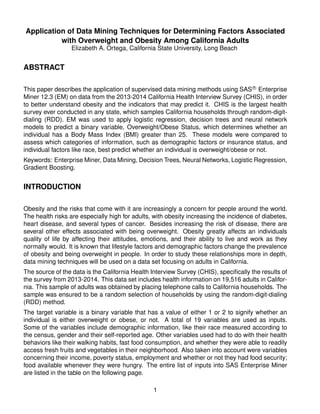
Application of Data Mining Techniques for Determining Factors Associated
with Overweight and Obesity Among California Adults
Elizabeth A. Ortega, California State University, Long Beach
ABSTRACT
This paper describes the application of supervised data mining methods using SAS R
Enterprise
Miner 12.3 (EM) on data from the 2013-2014 California Health Interview Survey (CHIS), in order
to better understand obesity and the indicators that may predict it. CHIS is the largest health
survey ever conducted in any state, which samples California households through random-digit-
dialing (RDD). EM was used to apply logistic regression, decision trees and neural network
models to predict a binary variable, Overweight/Obese Status, which determines whether an
individual has a Body Mass Index (BMI) greater than 25. These models were compared to
assess which categories of information, such as demographic factors or insurance status, and
individual factors like race, best predict whether an individual is overweight/obese or not.
Keywords: Enterprise Miner, Data Mining, Decision Trees, Neural Networks, Logistic Regression,
Gradient Boosting.
INTRODUCTION
Obesity and the risks that come with it are increasingly a concern for people around the world.
The health risks are especially high for adults, with obesity increasing the incidence of diabetes,
heart disease, and several types of cancer. Besides increasing the risk of disease, there are
several other effects associated with being overweight. Obesity greatly affects an individuals
quality of life by affecting their attitudes, emotions, and their ability to live and work as they
normally would. It is known that lifestyle factors and demographic factors change the prevalence
of obesity and being overweight in people. In order to study these relationships more in depth,
data mining techniques will be used on a data set focusing on adults in California.
The source of the data is the California Health Interview Survey (CHIS), specifically the results of
the survey from 2013-2014. This data set includes health information on 19,516 adults in Califor-
nia. This sample of adults was obtained by placing telephone calls to California households. The
sample was ensured to be a random selection of households by using the random-digit-dialing
(RDD) method.
The target variable is a binary variable that has a value of either 1 or 2 to signify whether an
individual is either overweight or obese, or not. A total of 19 variables are used as inputs.
Some of the variables include demographic information, like their race measured according to
the census, gender and their self-reported age. Other variables used had to do with their health
behaviors like their walking habits, fast food consumption, and whether they were able to readily
access fresh fruits and vegetables in their neighborhood. Also taken into account were variables
concerning their income, poverty status, employment and whether or not they had food security;
food available whenever they were hungry. The entire list of inputs into SAS Enterprise Miner
are listed in the table on the following page.
1
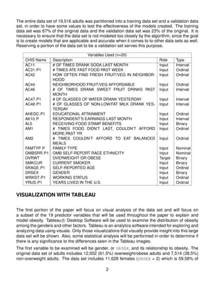
The entire data set of 19,516 adults was partitioned into a training data set and a validation data
set, in order to have some values to test the effectiveness of the models created. The training
data set was 67% of the original data and the validation data set was 23% of the original. It is
necessary to ensure that the data set is not modeled too closely by the algorithm, since the goal
is to create models that are applicable and accurate when it comes to to other data sets as well.
Reserving a portion of the data set to be a validation set serves this purpose.
Variables Used (n=20)
CHIS Name Description Role Type
AC11 # OF TIMES DRANK SODA LAST MONTH Input Interval
AC31 P1 # TIMES ATE FAST FOOD PAST WEEK Input Ordinal
AC42 HOW OFTEN FIND FRESH FRUIT/VEG IN NEIGHBOR-
HOOD
Input Ordinal
AC44 NEIGHBORHOOD FRUIT/VEG AFFORDABLE Input Ordinal
AC46 # OF TIMES DRANK SWEET FRUIT DRINKS PAST
MONTH
Input Interval
AC47 P1 # OF GLASSES OF WATER DRANK YESTERDAY Input Interval
AC48 P1 # OF GLASSES OF NON-LOW/FAT MILK DRANK YES-
TERDAY
Input Interval
AHEDC P1 EDUCATIONAL ATTAINMENT Input Ordinal
AK10 P RESPONDENT’S EARNINGS LAST MONTH Input Interval
AL5 RECEIVING FOOD STAMP BENEFITS Input Binary
AM1 # TIMES FOOD DIDN’T LAST, COULDN’T AFFORD
MORE,PAST YR
Input Ordinal
AM2 # TIMES COULDN’T AFFORD TO EAT BALANCED
MEALS
Input Ordinal
FAMTYP P FAMILY TYPE Input Nominal
OMBSRR P1 OMB SELF-REPORT RACE ETHNICITY Input Nominal
OVRWT OVERWEIGHT OR OBESE Target Binary
SMKCUR CURRENT SMOKER Input Binary
SRAGE P1 SELF-REPORTED AGE Input Ordinal
SRSEX GENDER Input Binary
WRKST P1 WORKING STATUS Input Ordinal
YRUS P1 YEARS LIVED IN THE U.S. Input Ordinal
VISUALIZATION WITH TABLEAU
The first portion of the paper will focus on visual analysis of the data set and will focus on
a subset of the 19 predictor variables that will be used throughout the paper to explain and
model obesity. Tableau R Desktop Software will be used to examine the distribution of obesity
among the genders and other factors. Tableau is an analytics software intended for exploring and
analyzing data using visuals. Only those visualizations that visually provide insight into this large
data set will be shown. Also, some statistical analysis will be performed in order to determine if
there is any significance to the differences seen in the Tableau images.
The first variable to be examined will be gender, or SRSEX, and its relationship to obesity. The
original data set of adults includes 12,002 (61.5%) overweight/obese adults and 7,514 (38.5%)
non-overweight adults. The data set includes 11,628 females (SRSEX = 2) which is 59.58% of
2
the data set and 7,888 males (SRSEX = 1) which is 40.42% of the data set. The figures below
show visually the original break down of gender in the data set and the original breakdown of
adults who have obese/overweight BMI values those who do not. It is important to keep in mind
when looking at future visualizations of this data that females outnumber males and there are
more overweight/obese people than adults who are not overweight.
The graphic below shows that there are more overweight/obese women in this data set than
overweight/obese men in this data set. However, it is important to keep the breakdown above in
mind.
However, the percentage of men that are obese is actually larger than the percentage of women
that are obese, as is shown in the tables below. If one had only seen the visualization above
they would have thought that women are obese/overweight more often than men, when it is
actually the other way around. A t test was used to see if the difference between the genders
was statistically significant. The test yielded a t value of -17.22 and a p value of <.0001, which
signifies that there is a significant difference in obesity between the genders.
3
Another factor that may play a part in obesity is age. In order to model this visually, the graph
below uses the binned self-report age variable SRAGE as well as the gender variable explored
earlier in order to examine the difference in obesity among different ages and genders.
The value shown on left signifies the lower boundary for the age variable bin. The blue bars,
which are represented by negative numbers on the axis, show the number of overweight/obese
men in the data set for that particular age bin. The pink bars show the same for women, which
are shown in positive numbers. It can be seen that the distribution of obesity by age is similar for
both genders, but obesity varies greatly with age.
Analysis of Variance (ANOVA) was used on the age groups to see if the groups did in fact differ in
terms of obesity. The F value found from this test was 31.34 and the corresponding p value was
<.0001. This result suggests that there is a statistical difference in obesity between the different
age groups.
Race is another demographic variable that may explain obesity in this population of adults. The
variable OMBSRR P1 self-report race and ethnicity according to the Office of Management and
Budget (OMB) standards. A value of 1 signifies that the indvidual’s race/ethnicity is Hispanic,
a value of 2 signifies that the individual is White, Non-Hispanic, a value of 3 signifies African-
American, a value of 4 signifies American Indian or Alaskan Native, a value of 5 signifies Asian,
6 represents Other and 7 signifies that the respondent identified with two or more races or
ethnicities.
The figure below shows a the distribution of overweight/obese, the 1 value on the left, and 0 not
obese, among the different races which are shown on the horizontal axis.
Those races which have a more equal distribution of obese/non-obese individuals have squares
which are similar in pigmentation. One race that shows this is 2, White Non-Hispanic, which
has almost as many non-obese individuals as obese ones. The races that have an unequal
distribution show one square as gray and one square as very red, like group 2, Hispanics. This
race has substantially more individuals who are overweight/obese than those who are not, with
73% of Hispanics in this group being overweight/obese.
4
An ANOVA analysis was also conducted on these groups and the resulting F statistic was 136.09
with a p value of <.0001, signifying that there is a substantial difference in the distribution of
obesity between the races.
From the graph below one can also see that group 5, Asians, has significantly more individuals
who are not overweight, than those who are. Overweight individuals make up only 37% of
the Asian adults sampled, almost the reverse of the distribution of obesity in the entire sample
including all races.
Also explored visually was the relationship between educational attainment and obesity. The
graphic below shows the distribution of obesity among the different levels of educational attain-
ment which range from 1,which signifies that the adult has had no formal education, to 10 which
signifies that the respondent holds a doctorate degree. The horizontal axis represents the num-
ber of overweight/obese adults in each of these educational categories. ANOVA was also used
to compare these groups and the results showed that there is a statistically significant different
in obesity among the different education levels. When comparing these groups to one another
using Bonferroni tests, there is a statistically significant difference between those who have grad-
uate degrees (master’s or doctorate degrees) and those who do not. Those who do not tend to
be obese/overweight more often than those who have graduate degrees.
DECISION TREES
The EM diagram shown below shows the different decision trees fit to the training data set and
tested for effectiveness with the validation data set.
5
In total, 5 types of decision tree algorithms were used on the data, as well as an interactive
decision tree and a gradient boosting decision tree. The first type of decision tree used was a
simple classification and regression tree (CART) algorithm, which is a binary decision tree that
constructs nodes and splits them based on Gini impurity. Gini impurity determines how often a
randomly chosen element would be labeled incorrectly if it were labeled randomly based on the
distribution of labels in the smaller subset. The formula for calculating the Gini index of a node
is below for a data set T with examples from n classes.
This CART tree yielded 10 significant variables, with race being the most important. The next
most important variable was the number of times an individual ate fast food in the last week. The
variables and their importance for this first tree are listed below. The decision tree diagram in its
entirety is also shown. The diagrams for the following trees are much more complicated, since
they are not binary and contain several more nodes than this tree so they will not be shown.
6
Since the original distribution of obesity/overweight in the original data set was 62% overweight/obese
and 38% not overweight or obese, below are some nodes that showed a significantly different
distribution of obesity than the original data. For example, Asian women have a significantly
lower risk of obesity with only 29.6% of them being overweight/obese and 70.4% being not over-
weight or obese.
A group that has an even higher rate of obesity than the original data set is the group that is
composed of Hispanics, African-Americans or American Indians that are older than 26 and eat
fast food more than once a week. This group has an 80.1% prevalence of obesity.
Tree 2 was the best tree in terms of the misclassification rate. It used the C4.5 algorithm with
a maximum of 4 branches. Instead of Gini impurity, the C4.5 algorithm uses entropy to decide
whether or not a node should be made. The formula for entropy is below:
7
This algorithm yielded 13 variables of importance, with race also being the most important vari-
able. The list of variables in order of importance is below. The misclassification rate was, for this
tree, .321 for the training data set and .332 for the validation data set.
The remaining trees did not follow a specific algorithm, besides the third tree that used the C4.5
algorithm but with a maximum of 6 branches, and they did not yield any significant increases in
ability to classify as Tree 4 so this is the last one I will list results for individually. This tree used
variance, entropy for nominal variables and Gini impurity for ordinal variables in order to classify
each of the nodes. The variables in order of importance are below. The variables used were 19,
so this tree used all of the available input variables in order to classify the data into groups. The
misclassification rate for this tree was .305 for training, .322 for validation.
8
GRADIENT BOOSTING
Gradient boosting is a method specifically for reducing error in decision trees. In this case we
are looking at the misclassification rate as our error rate, which is the number of predictions that
incorrectly predict the value of our target variable.
Error is not considered to be more important in either case, whether we misclassify an over-
weight/obese individual as not overweight or whether we classify a person who is not overweight
as overweight/obese. When comparing the best models from each method, we will consider
these more in detail, since it may be more important to correctly classify overweight/obese indi-
viduals.
DECISION TREES, CONTINUED
The remaining trees including the gradient boosting tree and excluding the interactive decision
tree because that one was made using user inputs in order to decide when to create a node and
in what order the variables were used, had several similarities. They are compared using the
model comparison tool in Enterprise Miner below. The ROC curves are shown for these models
for both the training and validation data sets.
Race was the most important variable in all of these decision trees, no matter the criterion used
to create the nodes. Age, gender, and fast food frequency were in the top 5 most important
variables in each of the trees, usually followed by earnings and educational attainment.
Following this were the variables on the subjects drinking habits: how often they had soda in the
last month, low fat or skim milk, sweet fruit drinks or how often they drank water. These variables
were usually clumped together but varied slightly in their order of importance from tree to tree.
The food security variables like whether or not a subject was using food stamp benefits, and
whether or not they always had food available to them when they were hungry were significant
in all trees, but always consistently at the bottom of the list in terms of significance.
This was surprising, since I expected these variables to contribute more heavily to whether or
not a subject was overweight or not. The misclassification rate for all of these trees was around
.32-.33 and did not change substantially from the training data set to the validation data set. As
can be seen in the ROC curves below for all the trees, Tree 4 seems to be the best and all of the
trees provide a substantial increase in classifying power from random chance.
9
CLUSTER ANALYSIS AS INPUT TO DECISION TREES
A decision tree was also used to model the different segments created using cluster analysis by
using a cluster node before a decision tree node and changing the target variable to SEGMENT
instead of OVRWT.
This method had a much lower misclassification rate than the decision trees without this feature,
however, these two types of decision trees are not comparable to one another. Using a decision
tree here just helps understand the different clusters created more clearly. For this data set, the
best amount of clusters was two.
On the training data this method had a .46 misclassification rate and a .56 rate on the validation
data set. When analyzing the cluster means and variables used (which were 17 of the original
19), a picture began to emerge of the types of adults in each of the clusters. Cluster 1 adults on
average only had soda and sweet drinks twice a month. These adults earned almost twice as
much monthly, on average, than the adults in Cluster 2. This cluster consisted mainly of females
and had more White and Asian adults than Cluster 2.
Cluster 2 on the other hand contained individuals who on average had soda 22 times a month
and 15 sweet drinks a month. Besides only making $1,200 a month, these individuals were
mainly males and were more likely to be Hispanic and current smokers than those in Cluster
1. Cluster 1 consisted of 84.38% of the data and Cluster 2 was 15.62%. The variables used
in the clustering and subsequent tree are shown below in order of importance as well as their
importance to the model.
10
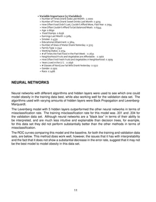
NEURAL NETWORKS
Neural networks with different algorithms and hidden layers were used to see which one could
model obesity in the training data best, while also working well for the validation data set. The
algorithms used with varying amounts of hidden layers were Back Propogation and Levenberg-
Marquardt.
The Levenberg model with 5 hidden layers outperformed the other neural networks in terms of
missclassification rate. The training misclassification rate for this model was .331 and .334 for
the validation data set. Although neural networks are a ”black box” in terms of their ability to
be interpreted, and are much less intuitive and explainable than decision trees, for example,
for this data set they did not perform substantially better than the other methods in terms of
missclassification.
The ROC curves comparing this model and the baseline, for both the training and validation data
sets, are below. This method does work well, however, the issues that it has with interpretability
and the fact that it does not show a substantial decrease in the error rate, suggest that it may not
be the best model to model obesity in this data set.
11
LOGISTIC REGRESSION
In order to determine whether these data mining techniques, which at times require large amounts
of computing power, offer substantial insight into our data set over traditional methods, logistic
regression models were fit to the data. The stepwise, forward and backward selection methods
were used find the best models for the training data, the models were also judged based on
misclassification rate. All of these selection methods yielded a model which was significant at
the α =.05 level.
The method selected using these procedures yielded a misclassification rate of .332 for the train-
ing data and .335 for the validation data. The Akaike’s Information Criterion (AIC) value for this
model is 16071.46. It includes the twelve following variables, all of which are significant at the α
=.05 level individually as predictors: Fast Food, Non-Low/Fat Milk, Educational Attainment, Food
Stamp Benefits, Couldn’t Afford Balanced Meals, Family Type, Race, Smoker, Age, Gender,
Working Status, Years Living in the U.S.
Overall, this classical method did not perform substantially differently than the data mining tech-
niques used on this data set. It seems that logistic regression is a good option for modeling
obesity in adults, especially because it is already familiar to most individuals in the health field,
where these data mining techniques may not be.
ERROR RATE COMPARISON
Comparing the classification charts for the best decision tree, logistic regression model and neu-
ral network, shows the differences in classification for each of the methods. All of the methods
had a higher rate of classifying individuals as overweight/obese versus not overweight. Also, all
three of the models had more observations that they incorrectly classified as overweight than
observations that were incorrectly classified as not overweight.
This is positive, since it is more beneficial that our model correctly identifies those who are
overweight/obese, since that is our focus. The models were similar in terms of the rates in which
12
they incorrectly and correctly classified the data. Below are the classification charts for the best
decision tree, neural network and logistic regression model, in that order, for the training data
set.
CONCLUSIONS
The best model overall, in terms of missclassification rate, was the decision tree model using a
variation of the C4.5 algorithm. It had the lowest misclassification rate for the training data set
and validation data set, which were .305 and .322 respectively. The best neural network model
was not far behind with misclassification rates of .331 and .334 for training and validation. The
best logistic regression model had rates of .332 and .335.
The data mining techniques had slightly lower error rates than the classical technique of logistic
regression, for predicting our target variable of whether an individual is obese/overweight or not.
However, the classical method still resulted in a model that was comparable to those using more
advanced techniques. It seems that for predicting obesity in this sample, logistic regression is a
viable option. This may be due to the relatively large sample which this study was based on and
the fact that the sample contained very little missing data for the predictors used.
Overall the same types of variables were significant in most of the techniques used. Overall, de-
mographic factors like gender, educational attainment and race were more significant predictors
of obesity, whereas factors which had to do with an individual’s health behaviors like their soda
drinking habits, were less significant. Although this study is limited, since only 19 variables about
the adults were used as inputs into the models, this may have implications for how physicians
and public health officials tackle the increasing issue that is obesity in the United States.
SAS and all other SAS Institute Inc. product or service names are registered trademarks or
trademarks of SAS Institute Inc. in the USA and other countries. R indicates USA registration.
Other brand and product names are trademarks of their respective companies.
13

More Related Content

Viewers also liked

Commercialisation of innov
Commercialisation of innovCommercialisation of innov
Commercialisation of innovEmil Slm
 
okoroafor catem fidelis cv5
okoroafor catem fidelis cv5okoroafor catem fidelis cv5
okoroafor catem fidelis cv5catem okoroafor
 
Tics resumen
Tics resumenTics resumen
Tics resumenPaulyamor
 
Quer Agrade, quer desagrade - Pe. Fernando A. Rifan
Quer Agrade, quer desagrade - Pe. Fernando A. RifanQuer Agrade, quer desagrade - Pe. Fernando A. Rifan
Quer Agrade, quer desagrade - Pe. Fernando A. RifanComplexo_Galaad
 
Presentación Profesional - Ximo Garcia
Presentación Profesional - Ximo GarciaPresentación Profesional - Ximo Garcia
Presentación Profesional - Ximo GarciaXimo García Parra
 
Samvel araqelyan rodari
Samvel araqelyan rodariSamvel araqelyan rodari
Samvel araqelyan rodariNaira Daluzyan
 

Viewers also liked (12)

Commercialisation of innov
Commercialisation of innovCommercialisation of innov
Commercialisation of innov
 
Elen
ElenElen
Elen
 
okoroafor catem fidelis cv5
okoroafor catem fidelis cv5okoroafor catem fidelis cv5
okoroafor catem fidelis cv5
 
Basic computer-skills1
Basic computer-skills1Basic computer-skills1
Basic computer-skills1
 
Layfield-Christopher-BHR-Baltimore-2014
Layfield-Christopher-BHR-Baltimore-2014Layfield-Christopher-BHR-Baltimore-2014
Layfield-Christopher-BHR-Baltimore-2014
 
Tics resumen
Tics resumenTics resumen
Tics resumen
 
Louvre
LouvreLouvre
Louvre
 
Quer Agrade, quer desagrade - Pe. Fernando A. Rifan
Quer Agrade, quer desagrade - Pe. Fernando A. RifanQuer Agrade, quer desagrade - Pe. Fernando A. Rifan
Quer Agrade, quer desagrade - Pe. Fernando A. Rifan
 
Presentación Profesional - Ximo Garcia
Presentación Profesional - Ximo GarciaPresentación Profesional - Ximo Garcia
Presentación Profesional - Ximo Garcia
 
Ravinder-1
Ravinder-1Ravinder-1
Ravinder-1
 
Samvel araqelyan rodari
Samvel araqelyan rodariSamvel araqelyan rodari
Samvel araqelyan rodari
 
Interferenciasoclusales 091113132025-phpapp01
Interferenciasoclusales 091113132025-phpapp01Interferenciasoclusales 091113132025-phpapp01
Interferenciasoclusales 091113132025-phpapp01
 

Similar to Final Data Mining_Elizabeth Ortega

Healthy Food Accessibility and Obesity: Case Study of Pennsylvania, USA
Healthy Food Accessibility and Obesity: Case Study of Pennsylvania, USAHealthy Food Accessibility and Obesity: Case Study of Pennsylvania, USA
Healthy Food Accessibility and Obesity: Case Study of Pennsylvania, USArsmahabir
 
Nutritional Status of Government school children
Nutritional Status of Government school childrenNutritional Status of Government school children
Nutritional Status of Government school childrenJohn Medley-Hallam
 
HtWt_Full-Report2006_Approved-Final
HtWt_Full-Report2006_Approved-FinalHtWt_Full-Report2006_Approved-Final
HtWt_Full-Report2006_Approved-FinalDr. Zeenat Mahal
 
PATH Report Northeast_NHS_UK
PATH Report Northeast_NHS_UKPATH Report Northeast_NHS_UK
PATH Report Northeast_NHS_UKFrederick Navarro
 
Uop mha 610 week 6 discussion health and nutritional status new
Uop mha 610 week 6 discussion health and nutritional status newUop mha 610 week 6 discussion health and nutritional status new
Uop mha 610 week 6 discussion health and nutritional status neweyavagal
 
Uop mha 610 week 6 discussion health and nutritional status new
Uop mha 610 week 6 discussion health and nutritional status newUop mha 610 week 6 discussion health and nutritional status new
Uop mha 610 week 6 discussion health and nutritional status neweyavagal
 
Uop mha 610 week 6 discussion health and nutritional status new
Uop mha 610 week 6 discussion health and nutritional status newUop mha 610 week 6 discussion health and nutritional status new
Uop mha 610 week 6 discussion health and nutritional status newshyaminfopvtltd
 
Uop mha 610 week 6 discussion health and nutritional status new
Uop mha 610 week 6 discussion health and nutritional status newUop mha 610 week 6 discussion health and nutritional status new
Uop mha 610 week 6 discussion health and nutritional status newNoahliamwilliam
 
Marissa Menendez Major Project Paper 1-30-15
Marissa Menendez Major Project Paper 1-30-15Marissa Menendez Major Project Paper 1-30-15
Marissa Menendez Major Project Paper 1-30-15Marissa Menendez
 
Hutchinson and holtman, 2005
Hutchinson and holtman, 2005Hutchinson and holtman, 2005
Hutchinson and holtman, 2005Quyen Nguyen
 
Open data analysis using business intelligence tools
Open data analysis using business intelligence toolsOpen data analysis using business intelligence tools
Open data analysis using business intelligence toolsService_supportAssignment
 
The American Journal of Clinical Nutrition - ¿Sabemos todo sobre las bebidas ...
The American Journal of Clinical Nutrition - ¿Sabemos todo sobre las bebidas ...The American Journal of Clinical Nutrition - ¿Sabemos todo sobre las bebidas ...
The American Journal of Clinical Nutrition - ¿Sabemos todo sobre las bebidas ...claudiadelbosque
 
8141410.pptbbbbbbbnnnnnnnnnnnnnnnnnnnnnnnnnnnnnnnnnnnnnnnnnnnnnnnnnnnnnnnnnnn
8141410.pptbbbbbbbnnnnnnnnnnnnnnnnnnnnnnnnnnnnnnnnnnnnnnnnnnnnnnnnnnnnnnnnnnn8141410.pptbbbbbbbnnnnnnnnnnnnnnnnnnnnnnnnnnnnnnnnnnnnnnnnnnnnnnnnnnnnnnnnnnn
8141410.pptbbbbbbbnnnnnnnnnnnnnnnnnnnnnnnnnnnnnnnnnnnnnnnnnnnnnnnnnnnnnnnnnnnmhosn627
 
Obesity and Physical Activity & SRH Poster
Obesity and Physical Activity & SRH PosterObesity and Physical Activity & SRH Poster
Obesity and Physical Activity & SRH PosterErin Flores, MPH
 
Assessment and Treatment of Childhood Obesity
Assessment and Treatment of Childhood ObesityAssessment and Treatment of Childhood Obesity
Assessment and Treatment of Childhood ObesityHEALTHCoalition
 
Body Weight, Diabetes, and Access to Nutritious Food
Body Weight, Diabetes, and Access to Nutritious Food Body Weight, Diabetes, and Access to Nutritious Food
Body Weight, Diabetes, and Access to Nutritious Food Phylicia Morgan
 

Similar to Final Data Mining_Elizabeth Ortega (20)

Healthy Food Accessibility and Obesity: Case Study of Pennsylvania, USA
Healthy Food Accessibility and Obesity: Case Study of Pennsylvania, USAHealthy Food Accessibility and Obesity: Case Study of Pennsylvania, USA
Healthy Food Accessibility and Obesity: Case Study of Pennsylvania, USA
 
Nutritional Status of Government school children
Nutritional Status of Government school childrenNutritional Status of Government school children
Nutritional Status of Government school children
 
HtWt_Full-Report2006_Approved-Final
HtWt_Full-Report2006_Approved-FinalHtWt_Full-Report2006_Approved-Final
HtWt_Full-Report2006_Approved-Final
 
PATH Report Northeast_NHS_UK
PATH Report Northeast_NHS_UKPATH Report Northeast_NHS_UK
PATH Report Northeast_NHS_UK
 
Uop mha 610 week 6 discussion health and nutritional status new
Uop mha 610 week 6 discussion health and nutritional status newUop mha 610 week 6 discussion health and nutritional status new
Uop mha 610 week 6 discussion health and nutritional status new
 
Uop mha 610 week 6 discussion health and nutritional status new
Uop mha 610 week 6 discussion health and nutritional status newUop mha 610 week 6 discussion health and nutritional status new
Uop mha 610 week 6 discussion health and nutritional status new
 
Uop mha 610 week 6 discussion health and nutritional status new
Uop mha 610 week 6 discussion health and nutritional status newUop mha 610 week 6 discussion health and nutritional status new
Uop mha 610 week 6 discussion health and nutritional status new
 
Uop mha 610 week 6 discussion health and nutritional status new
Uop mha 610 week 6 discussion health and nutritional status newUop mha 610 week 6 discussion health and nutritional status new
Uop mha 610 week 6 discussion health and nutritional status new
 
Marissa Menendez Major Project Paper 1-30-15
Marissa Menendez Major Project Paper 1-30-15Marissa Menendez Major Project Paper 1-30-15
Marissa Menendez Major Project Paper 1-30-15
 
Anthropometric worldbank
Anthropometric worldbankAnthropometric worldbank
Anthropometric worldbank
 
Hutchinson and holtman, 2005
Hutchinson and holtman, 2005Hutchinson and holtman, 2005
Hutchinson and holtman, 2005
 
Open data analysis using business intelligence tools
Open data analysis using business intelligence toolsOpen data analysis using business intelligence tools
Open data analysis using business intelligence tools
 
jgi_01104.pdf
jgi_01104.pdfjgi_01104.pdf
jgi_01104.pdf
 
The American Journal of Clinical Nutrition - ¿Sabemos todo sobre las bebidas ...
The American Journal of Clinical Nutrition - ¿Sabemos todo sobre las bebidas ...The American Journal of Clinical Nutrition - ¿Sabemos todo sobre las bebidas ...
The American Journal of Clinical Nutrition - ¿Sabemos todo sobre las bebidas ...
 
8141410.pptbbbbbbbnnnnnnnnnnnnnnnnnnnnnnnnnnnnnnnnnnnnnnnnnnnnnnnnnnnnnnnnnnn
8141410.pptbbbbbbbnnnnnnnnnnnnnnnnnnnnnnnnnnnnnnnnnnnnnnnnnnnnnnnnnnnnnnnnnnn8141410.pptbbbbbbbnnnnnnnnnnnnnnnnnnnnnnnnnnnnnnnnnnnnnnnnnnnnnnnnnnnnnnnnnnn
8141410.pptbbbbbbbnnnnnnnnnnnnnnnnnnnnnnnnnnnnnnnnnnnnnnnnnnnnnnnnnnnnnnnnnnn
 
CUN-BAE PDF
CUN-BAE PDFCUN-BAE PDF
CUN-BAE PDF
 
Obesity and Physical Activity & SRH Poster
Obesity and Physical Activity & SRH PosterObesity and Physical Activity & SRH Poster
Obesity and Physical Activity & SRH Poster
 
Assessment and Treatment of Childhood Obesity
Assessment and Treatment of Childhood ObesityAssessment and Treatment of Childhood Obesity
Assessment and Treatment of Childhood Obesity
 
BEHEP Health Disparity Conference
BEHEP Health Disparity ConferenceBEHEP Health Disparity Conference
BEHEP Health Disparity Conference
 
Body Weight, Diabetes, and Access to Nutritious Food
Body Weight, Diabetes, and Access to Nutritious Food Body Weight, Diabetes, and Access to Nutritious Food
Body Weight, Diabetes, and Access to Nutritious Food
 

Final Data Mining_Elizabeth Ortega

  • 1. Application of Data Mining Techniques for Determining Factors Associated with Overweight and Obesity Among California Adults Elizabeth A. Ortega, California State University, Long Beach ABSTRACT This paper describes the application of supervised data mining methods using SAS R Enterprise Miner 12.3 (EM) on data from the 2013-2014 California Health Interview Survey (CHIS), in order to better understand obesity and the indicators that may predict it. CHIS is the largest health survey ever conducted in any state, which samples California households through random-digit- dialing (RDD). EM was used to apply logistic regression, decision trees and neural network models to predict a binary variable, Overweight/Obese Status, which determines whether an individual has a Body Mass Index (BMI) greater than 25. These models were compared to assess which categories of information, such as demographic factors or insurance status, and individual factors like race, best predict whether an individual is overweight/obese or not. Keywords: Enterprise Miner, Data Mining, Decision Trees, Neural Networks, Logistic Regression, Gradient Boosting. INTRODUCTION Obesity and the risks that come with it are increasingly a concern for people around the world. The health risks are especially high for adults, with obesity increasing the incidence of diabetes, heart disease, and several types of cancer. Besides increasing the risk of disease, there are several other effects associated with being overweight. Obesity greatly affects an individuals quality of life by affecting their attitudes, emotions, and their ability to live and work as they normally would. It is known that lifestyle factors and demographic factors change the prevalence of obesity and being overweight in people. In order to study these relationships more in depth, data mining techniques will be used on a data set focusing on adults in California. The source of the data is the California Health Interview Survey (CHIS), specifically the results of the survey from 2013-2014. This data set includes health information on 19,516 adults in Califor- nia. This sample of adults was obtained by placing telephone calls to California households. The sample was ensured to be a random selection of households by using the random-digit-dialing (RDD) method. The target variable is a binary variable that has a value of either 1 or 2 to signify whether an individual is either overweight or obese, or not. A total of 19 variables are used as inputs. Some of the variables include demographic information, like their race measured according to the census, gender and their self-reported age. Other variables used had to do with their health behaviors like their walking habits, fast food consumption, and whether they were able to readily access fresh fruits and vegetables in their neighborhood. Also taken into account were variables concerning their income, poverty status, employment and whether or not they had food security; food available whenever they were hungry. The entire list of inputs into SAS Enterprise Miner are listed in the table on the following page. 1
  • 2. The entire data set of 19,516 adults was partitioned into a training data set and a validation data set, in order to have some values to test the effectiveness of the models created. The training data set was 67% of the original data and the validation data set was 23% of the original. It is necessary to ensure that the data set is not modeled too closely by the algorithm, since the goal is to create models that are applicable and accurate when it comes to to other data sets as well. Reserving a portion of the data set to be a validation set serves this purpose. Variables Used (n=20) CHIS Name Description Role Type AC11 # OF TIMES DRANK SODA LAST MONTH Input Interval AC31 P1 # TIMES ATE FAST FOOD PAST WEEK Input Ordinal AC42 HOW OFTEN FIND FRESH FRUIT/VEG IN NEIGHBOR- HOOD Input Ordinal AC44 NEIGHBORHOOD FRUIT/VEG AFFORDABLE Input Ordinal AC46 # OF TIMES DRANK SWEET FRUIT DRINKS PAST MONTH Input Interval AC47 P1 # OF GLASSES OF WATER DRANK YESTERDAY Input Interval AC48 P1 # OF GLASSES OF NON-LOW/FAT MILK DRANK YES- TERDAY Input Interval AHEDC P1 EDUCATIONAL ATTAINMENT Input Ordinal AK10 P RESPONDENT’S EARNINGS LAST MONTH Input Interval AL5 RECEIVING FOOD STAMP BENEFITS Input Binary AM1 # TIMES FOOD DIDN’T LAST, COULDN’T AFFORD MORE,PAST YR Input Ordinal AM2 # TIMES COULDN’T AFFORD TO EAT BALANCED MEALS Input Ordinal FAMTYP P FAMILY TYPE Input Nominal OMBSRR P1 OMB SELF-REPORT RACE ETHNICITY Input Nominal OVRWT OVERWEIGHT OR OBESE Target Binary SMKCUR CURRENT SMOKER Input Binary SRAGE P1 SELF-REPORTED AGE Input Ordinal SRSEX GENDER Input Binary WRKST P1 WORKING STATUS Input Ordinal YRUS P1 YEARS LIVED IN THE U.S. Input Ordinal VISUALIZATION WITH TABLEAU The first portion of the paper will focus on visual analysis of the data set and will focus on a subset of the 19 predictor variables that will be used throughout the paper to explain and model obesity. Tableau R Desktop Software will be used to examine the distribution of obesity among the genders and other factors. Tableau is an analytics software intended for exploring and analyzing data using visuals. Only those visualizations that visually provide insight into this large data set will be shown. Also, some statistical analysis will be performed in order to determine if there is any significance to the differences seen in the Tableau images. The first variable to be examined will be gender, or SRSEX, and its relationship to obesity. The original data set of adults includes 12,002 (61.5%) overweight/obese adults and 7,514 (38.5%) non-overweight adults. The data set includes 11,628 females (SRSEX = 2) which is 59.58% of 2
  • 3. the data set and 7,888 males (SRSEX = 1) which is 40.42% of the data set. The figures below show visually the original break down of gender in the data set and the original breakdown of adults who have obese/overweight BMI values those who do not. It is important to keep in mind when looking at future visualizations of this data that females outnumber males and there are more overweight/obese people than adults who are not overweight. The graphic below shows that there are more overweight/obese women in this data set than overweight/obese men in this data set. However, it is important to keep the breakdown above in mind. However, the percentage of men that are obese is actually larger than the percentage of women that are obese, as is shown in the tables below. If one had only seen the visualization above they would have thought that women are obese/overweight more often than men, when it is actually the other way around. A t test was used to see if the difference between the genders was statistically significant. The test yielded a t value of -17.22 and a p value of <.0001, which signifies that there is a significant difference in obesity between the genders. 3
  • 4. Another factor that may play a part in obesity is age. In order to model this visually, the graph below uses the binned self-report age variable SRAGE as well as the gender variable explored earlier in order to examine the difference in obesity among different ages and genders. The value shown on left signifies the lower boundary for the age variable bin. The blue bars, which are represented by negative numbers on the axis, show the number of overweight/obese men in the data set for that particular age bin. The pink bars show the same for women, which are shown in positive numbers. It can be seen that the distribution of obesity by age is similar for both genders, but obesity varies greatly with age. Analysis of Variance (ANOVA) was used on the age groups to see if the groups did in fact differ in terms of obesity. The F value found from this test was 31.34 and the corresponding p value was <.0001. This result suggests that there is a statistical difference in obesity between the different age groups. Race is another demographic variable that may explain obesity in this population of adults. The variable OMBSRR P1 self-report race and ethnicity according to the Office of Management and Budget (OMB) standards. A value of 1 signifies that the indvidual’s race/ethnicity is Hispanic, a value of 2 signifies that the individual is White, Non-Hispanic, a value of 3 signifies African- American, a value of 4 signifies American Indian or Alaskan Native, a value of 5 signifies Asian, 6 represents Other and 7 signifies that the respondent identified with two or more races or ethnicities. The figure below shows a the distribution of overweight/obese, the 1 value on the left, and 0 not obese, among the different races which are shown on the horizontal axis. Those races which have a more equal distribution of obese/non-obese individuals have squares which are similar in pigmentation. One race that shows this is 2, White Non-Hispanic, which has almost as many non-obese individuals as obese ones. The races that have an unequal distribution show one square as gray and one square as very red, like group 2, Hispanics. This race has substantially more individuals who are overweight/obese than those who are not, with 73% of Hispanics in this group being overweight/obese. 4
  • 5. An ANOVA analysis was also conducted on these groups and the resulting F statistic was 136.09 with a p value of <.0001, signifying that there is a substantial difference in the distribution of obesity between the races. From the graph below one can also see that group 5, Asians, has significantly more individuals who are not overweight, than those who are. Overweight individuals make up only 37% of the Asian adults sampled, almost the reverse of the distribution of obesity in the entire sample including all races. Also explored visually was the relationship between educational attainment and obesity. The graphic below shows the distribution of obesity among the different levels of educational attain- ment which range from 1,which signifies that the adult has had no formal education, to 10 which signifies that the respondent holds a doctorate degree. The horizontal axis represents the num- ber of overweight/obese adults in each of these educational categories. ANOVA was also used to compare these groups and the results showed that there is a statistically significant different in obesity among the different education levels. When comparing these groups to one another using Bonferroni tests, there is a statistically significant difference between those who have grad- uate degrees (master’s or doctorate degrees) and those who do not. Those who do not tend to be obese/overweight more often than those who have graduate degrees. DECISION TREES The EM diagram shown below shows the different decision trees fit to the training data set and tested for effectiveness with the validation data set. 5
  • 6. In total, 5 types of decision tree algorithms were used on the data, as well as an interactive decision tree and a gradient boosting decision tree. The first type of decision tree used was a simple classification and regression tree (CART) algorithm, which is a binary decision tree that constructs nodes and splits them based on Gini impurity. Gini impurity determines how often a randomly chosen element would be labeled incorrectly if it were labeled randomly based on the distribution of labels in the smaller subset. The formula for calculating the Gini index of a node is below for a data set T with examples from n classes. This CART tree yielded 10 significant variables, with race being the most important. The next most important variable was the number of times an individual ate fast food in the last week. The variables and their importance for this first tree are listed below. The decision tree diagram in its entirety is also shown. The diagrams for the following trees are much more complicated, since they are not binary and contain several more nodes than this tree so they will not be shown. 6
  • 7. Since the original distribution of obesity/overweight in the original data set was 62% overweight/obese and 38% not overweight or obese, below are some nodes that showed a significantly different distribution of obesity than the original data. For example, Asian women have a significantly lower risk of obesity with only 29.6% of them being overweight/obese and 70.4% being not over- weight or obese. A group that has an even higher rate of obesity than the original data set is the group that is composed of Hispanics, African-Americans or American Indians that are older than 26 and eat fast food more than once a week. This group has an 80.1% prevalence of obesity. Tree 2 was the best tree in terms of the misclassification rate. It used the C4.5 algorithm with a maximum of 4 branches. Instead of Gini impurity, the C4.5 algorithm uses entropy to decide whether or not a node should be made. The formula for entropy is below: 7
  • 8. This algorithm yielded 13 variables of importance, with race also being the most important vari- able. The list of variables in order of importance is below. The misclassification rate was, for this tree, .321 for the training data set and .332 for the validation data set. The remaining trees did not follow a specific algorithm, besides the third tree that used the C4.5 algorithm but with a maximum of 6 branches, and they did not yield any significant increases in ability to classify as Tree 4 so this is the last one I will list results for individually. This tree used variance, entropy for nominal variables and Gini impurity for ordinal variables in order to classify each of the nodes. The variables in order of importance are below. The variables used were 19, so this tree used all of the available input variables in order to classify the data into groups. The misclassification rate for this tree was .305 for training, .322 for validation. 8
  • 9. GRADIENT BOOSTING Gradient boosting is a method specifically for reducing error in decision trees. In this case we are looking at the misclassification rate as our error rate, which is the number of predictions that incorrectly predict the value of our target variable. Error is not considered to be more important in either case, whether we misclassify an over- weight/obese individual as not overweight or whether we classify a person who is not overweight as overweight/obese. When comparing the best models from each method, we will consider these more in detail, since it may be more important to correctly classify overweight/obese indi- viduals. DECISION TREES, CONTINUED The remaining trees including the gradient boosting tree and excluding the interactive decision tree because that one was made using user inputs in order to decide when to create a node and in what order the variables were used, had several similarities. They are compared using the model comparison tool in Enterprise Miner below. The ROC curves are shown for these models for both the training and validation data sets. Race was the most important variable in all of these decision trees, no matter the criterion used to create the nodes. Age, gender, and fast food frequency were in the top 5 most important variables in each of the trees, usually followed by earnings and educational attainment. Following this were the variables on the subjects drinking habits: how often they had soda in the last month, low fat or skim milk, sweet fruit drinks or how often they drank water. These variables were usually clumped together but varied slightly in their order of importance from tree to tree. The food security variables like whether or not a subject was using food stamp benefits, and whether or not they always had food available to them when they were hungry were significant in all trees, but always consistently at the bottom of the list in terms of significance. This was surprising, since I expected these variables to contribute more heavily to whether or not a subject was overweight or not. The misclassification rate for all of these trees was around .32-.33 and did not change substantially from the training data set to the validation data set. As can be seen in the ROC curves below for all the trees, Tree 4 seems to be the best and all of the trees provide a substantial increase in classifying power from random chance. 9
  • 10. CLUSTER ANALYSIS AS INPUT TO DECISION TREES A decision tree was also used to model the different segments created using cluster analysis by using a cluster node before a decision tree node and changing the target variable to SEGMENT instead of OVRWT. This method had a much lower misclassification rate than the decision trees without this feature, however, these two types of decision trees are not comparable to one another. Using a decision tree here just helps understand the different clusters created more clearly. For this data set, the best amount of clusters was two. On the training data this method had a .46 misclassification rate and a .56 rate on the validation data set. When analyzing the cluster means and variables used (which were 17 of the original 19), a picture began to emerge of the types of adults in each of the clusters. Cluster 1 adults on average only had soda and sweet drinks twice a month. These adults earned almost twice as much monthly, on average, than the adults in Cluster 2. This cluster consisted mainly of females and had more White and Asian adults than Cluster 2. Cluster 2 on the other hand contained individuals who on average had soda 22 times a month and 15 sweet drinks a month. Besides only making $1,200 a month, these individuals were mainly males and were more likely to be Hispanic and current smokers than those in Cluster 1. Cluster 1 consisted of 84.38% of the data and Cluster 2 was 15.62%. The variables used in the clustering and subsequent tree are shown below in order of importance as well as their importance to the model. 10
  • 11. NEURAL NETWORKS Neural networks with different algorithms and hidden layers were used to see which one could model obesity in the training data best, while also working well for the validation data set. The algorithms used with varying amounts of hidden layers were Back Propogation and Levenberg- Marquardt. The Levenberg model with 5 hidden layers outperformed the other neural networks in terms of missclassification rate. The training misclassification rate for this model was .331 and .334 for the validation data set. Although neural networks are a ”black box” in terms of their ability to be interpreted, and are much less intuitive and explainable than decision trees, for example, for this data set they did not perform substantially better than the other methods in terms of missclassification. The ROC curves comparing this model and the baseline, for both the training and validation data sets, are below. This method does work well, however, the issues that it has with interpretability and the fact that it does not show a substantial decrease in the error rate, suggest that it may not be the best model to model obesity in this data set. 11
  • 12. LOGISTIC REGRESSION In order to determine whether these data mining techniques, which at times require large amounts of computing power, offer substantial insight into our data set over traditional methods, logistic regression models were fit to the data. The stepwise, forward and backward selection methods were used find the best models for the training data, the models were also judged based on misclassification rate. All of these selection methods yielded a model which was significant at the α =.05 level. The method selected using these procedures yielded a misclassification rate of .332 for the train- ing data and .335 for the validation data. The Akaike’s Information Criterion (AIC) value for this model is 16071.46. It includes the twelve following variables, all of which are significant at the α =.05 level individually as predictors: Fast Food, Non-Low/Fat Milk, Educational Attainment, Food Stamp Benefits, Couldn’t Afford Balanced Meals, Family Type, Race, Smoker, Age, Gender, Working Status, Years Living in the U.S. Overall, this classical method did not perform substantially differently than the data mining tech- niques used on this data set. It seems that logistic regression is a good option for modeling obesity in adults, especially because it is already familiar to most individuals in the health field, where these data mining techniques may not be. ERROR RATE COMPARISON Comparing the classification charts for the best decision tree, logistic regression model and neu- ral network, shows the differences in classification for each of the methods. All of the methods had a higher rate of classifying individuals as overweight/obese versus not overweight. Also, all three of the models had more observations that they incorrectly classified as overweight than observations that were incorrectly classified as not overweight. This is positive, since it is more beneficial that our model correctly identifies those who are overweight/obese, since that is our focus. The models were similar in terms of the rates in which 12
  • 13. they incorrectly and correctly classified the data. Below are the classification charts for the best decision tree, neural network and logistic regression model, in that order, for the training data set. CONCLUSIONS The best model overall, in terms of missclassification rate, was the decision tree model using a variation of the C4.5 algorithm. It had the lowest misclassification rate for the training data set and validation data set, which were .305 and .322 respectively. The best neural network model was not far behind with misclassification rates of .331 and .334 for training and validation. The best logistic regression model had rates of .332 and .335. The data mining techniques had slightly lower error rates than the classical technique of logistic regression, for predicting our target variable of whether an individual is obese/overweight or not. However, the classical method still resulted in a model that was comparable to those using more advanced techniques. It seems that for predicting obesity in this sample, logistic regression is a viable option. This may be due to the relatively large sample which this study was based on and the fact that the sample contained very little missing data for the predictors used. Overall the same types of variables were significant in most of the techniques used. Overall, de- mographic factors like gender, educational attainment and race were more significant predictors of obesity, whereas factors which had to do with an individual’s health behaviors like their soda drinking habits, were less significant. Although this study is limited, since only 19 variables about the adults were used as inputs into the models, this may have implications for how physicians and public health officials tackle the increasing issue that is obesity in the United States. SAS and all other SAS Institute Inc. product or service names are registered trademarks or trademarks of SAS Institute Inc. in the USA and other countries. R indicates USA registration. Other brand and product names are trademarks of their respective companies. 13