1. Aging influences the physiology of all tissues in an organism. Many of the intrinsic and
extrinsic factors that affect function in aging are common to all cells and tissues. The male
reproductive system of the fruit fly, Drosophila melanogaster, offers an attractive model to study
influences of aging because it is not essential to viability and is highly active. It is established that
environmental factors, such as food quality, temperature, and humidity, influence Drosophila fertility.
However, little is known about the extrinsic factors that control reproductive maintenance during
aging. The goal of this project is to determine other environmental sources that cause variation in
reproductive lifespan. To identify these causes of variation, length of fertility was analyzed using
established strains of flies from the Drosophila Genetic Reference Panel (DGRP). The DGRP is a
collection of lines derived from wild caught females that have been inbred until all flies within a line
are genetically identical. This allows little to no genetic variation. This allows for the manipulation of
Wolbachia on the sex chromosomes. Because individuals within a line are genetically identical, it is
expected that any differences between animals in the same line should be due to environmental
effects. Wolbachia is an infection that can be inherited through the sex gene. More specifically, it is a
bacterial infection that can be treated with a simple antibiotic, Tetracycline. Part of the goal of this
experiment will be to se how Wolbachia and treatments for Wolbachia affect the variation of the data.
Of the environmental parameters, culturing conditions were also kept constant, including size and
type of container, food source, and temperature. However, because different individuals performed
experimental manipulations of animals with different equipment at different times of day, variability
could result from those parameters. Preliminary analysis indicates that there is substantial variation
in reproductive lifespan among individual males from the same line. Comparisons of the influences of
specific experimenters, equipment, and time of day will be presented. Environmental factors
identified as regulating reproductive lifespan may also have influences on other aging tissues.
In conclusion, no one environmental factor was found that can explain the variation in reproductive lifespan
of the fruit flies. Further research into other environmental factors (The amount of food in the vial and carbon
dioxide exposure amount) along with an expanded study to include more data points would be the next steps for this
research. Pinpointing the sources of variation in the reproductive lifespan of these genetically similar fly lines could
increase research quality for all research that uses the lines. It can allow for less question about the results that were
found and reduce error. It could also provide insight into how much of a role the environment plays in the life of a
fruit fly. That could then be extrapolated out to hypothesize the effect of the environment on other species, including
humans.
Contribution of experimental assay conditions to the measurement of
reproductive lifespan in Drosophila melanogaster
Mary Lee, Jalen Hickman, Mariah Koehler, Eileen Ramirez, Kiyana Hinton, Nicholas McVay, Autumn Conger, Macy Minix, Ebrima
Jarju, Nicaia Nash, Michelle Giedt, Peter Mirabito, Douglas Harrison
Department of Biology, University of Kentucky, Lexington, KY
Introduction
Conclusion
Results and Discussion
Figure 2: Variation in Fertility Length Between Sections- Variation can be seen between
sections even though the lines are genetically similar, demonstrating that there are environmental factors
affecting the reproductive cycle length. A)The mean for each line was calculated for each section of
students. The means are shown plotted beside each other with each section having its own color bar. B)
The standard deviation for each line was also calculated for each section. Standard deviations were then
graphed beside each other with each section having its own color bar.
Figure 3: Variation by Line of the Reproductive Lifespan Assay
Graphs A and B a strip plot of all of the data that was collected in the experiment. This figure is to show the variation that occurs between the lines of the Drosophila
melanogaster. A strip plot was chosen over a graph with the average because it shows the range and variability. A) Shows the variation in lines and the variation in
treated and untreated lines. B) Show the variation in lines and the variation in the Infected and cured. Both graphs A and B in figure 2 typically show a large amount of
variation no matter the treatment that was received. Graphs C and D show standard deviation, so the spread of the data could be observed. Graph C shows the spread
of the infected and cured flies by line. Graph D shows the spread of the treated and untreated flies by the line. There does not appear to be a significant difference
between the lines or the treatments. It is important to note that the populations vary widely throughout the data.
Each researcher had one station with a set of flies. The first trail was a set of 12 flies, and the
second trial was a set of 18 flies. Virgin females were anesthetized using carbon dioxide and then
placed in each vial with two females per vial. The students would then place one male in each vial
already containing virgin females. Then, as shown in Figure 1, the crosses were continued until each
male failed to produce offspring for two crosses or died before becoming infertile. There were
different treatments given to different lines of flies. The first two treatment types are Infected and
cured. The first fly of this category will have the Wolbachia infection, but the second line will not
because it will have been given a dose of Tetracycline to fight off the Wolbachia infection. The second
group is the treated and untreated group. This group will have lines that are treated with Tetracycline
to get rid or the Wolbachia infection. The untreated group will not have Wolbachia either, but will not
have received any Tetracycline treatments.
Reproduc ve Lifespan Assay
X
X
X
Original ♂
X
X
Reproduc ve
Lifespan
1♂
2 new♂
Original ♂ 2 new♂
Original ♂ 2 new♂
2 new♂Original ♂
Day 0
Day 2
Day 4
Day n
Day n+2
Fer le
Fer le
Fer le
X
X
2 ♂
Infer le
Fer le
Figure 1: In order to determine the reproductive
lifespan of the male flies, one male was mated
with two virgin females for every cross. The
original males flies were then transferred to a
new tube containing two new virgins, around
every two days. This process was repeated until
the original male fly was no longer fertile for two
consecutive crosses that were negative for a
week, or until death.
!5#
0#
5#
10#
15#
20#
25#
30#
307#treated#307#untreated#391#treated#391#untreated#399#treated#399#untreated#765#treated#765#untreated#
Trial#1#
Trial#2#
!5#
0#
5#
10#
15#
20#
25#
30#
360#cured# 360#
infected#
380#cured# 380#
infected#
786#cured# 786#
infected#
820##cured# 820#
infected#
Trial#1#
Trial#2#
A B
A comparison be done between lines that were infected with Wolbachia and cured of the bacteria
infection. A strip plot of each of the data points can also be seen in Figure 2. Lines 360, 820, and
380 all have relatively similar amounts of variation regardless of the line being infected or
cured. Line 786 shows a large difference in variation with the infected version of the line having
data points clustered toward the low end. The treated version of the line, however, shows a large
spread in data points. These conclusions are upheld by a comparison of standard deviations
among the lines as shown by graph D in Figure 2. The standard deviations for lines 360, 820, and
380 are all similar when comparing the standard deviation of the cured and infected versions of the
lines. The standard deviations for line 786 were very different with the standard deviation of the
infected line being much lower than the standard deviation of the cured line. Because a large
difference in variation was only seen in one line, it cannot be concluded that the curing of Wolbachia
changes the variability of the reproductive lifespan of fruit flies.
A strip plot of the data reveals that between the untreated and treated version of lines 307, 391, and
399 there were differing levels of variation. For lines 307 and 391, the untreated version had more
variation in reproductive lifespan than the treated version as evidenced by more spread out data
points. In line 399, the treated version of the line had more variability than the untreated
version. Line 765 appears to have no noticeable difference in variation of reproductive lifespan
when examining the strip plot. So, although there seem to be obvious differences in the strip plot
there are not concrete patterns that can be observed. A comparison of the standard deviation of the
four lines further reveals this relationship for lines 307 and 399 by showing a difference in standard
deviation. The relationship is also confirmed as line 765 has similar standard deviations for both
versions of the line. Line 391, however, has very similar standard deviations, even though the strip
plot shows a large variation in data points. This similarity could be due to the clustering of the 391
untreated data points at the high and low ends of the reproductive lifespan length. This clustering
may have led to the standard deviation being more similar to the standard deviation of the more
compacted data of the treated version of the line. Because a decrease in variation with the use of
antibiotics was only seen in two of the four line comparisons, it is not certain that usage of antibiotics
to treat fruit flies decreases variation in reproductive lifespan among a line
.
Variation can also be examined by comparing the differing sections of classes that performed fly
crosses. As a result of each section meeting at a different time during the day, it is possible that this
factor affected variation in the reproductive lifespan of the fruit flies, so another comparison of the
mean reproductive lifespans of the same line of flies but with differing sections reveals that for line 307
untreated, 360 infected, 391 treated, 786 infected, and 820 infected there was a large difference in
means between sections. These differences can be seen in Figure 3, graph A. Further comparison of
the standard deviations of each line for each section reveals some differences between sections, but
no differences as large as the means. Because it is only the means that differ and not the standard
deviations, it is unlikely that there is much variation in reproductive lifespan among sections.
Another way to examine the variation among the lines is to look at the variation seen when comparing
the treated to untreated lines. As can be seen in Figure 2, there was definitely noticeable variation in
the length of the reproductive lifespan throughout the line. A strip plot of the data reveals that between
the untreated and treated version of lines 307, 391, and 399 there were differing levels of
variation. For lines 307 and 391, the untreated version had more variation in reproductive lifespan
than the treated version as evidenced by more spread out data points. In line 399, the treated version
of the line had more variability than the untreated version. Line 765 appears to have no noticeable
difference in variation of reproductive lifespan when examining the strip plot. A comparison of the
standard deviation of the four lines further reveals this relationship for lines 307 and 399 by showing a
difference in standard deviation. The relationship is also confirmed as line 765 has similar standard
deviations for both versions of the line. Line 391, however, has very similar standard deviations, even
though the strip plot shows a large variation in data points. This similarity could be due to the
clustering of the 391 untreated data points at the high and low ends of the reproductive lifespan
length. This clustering may have led to the standard deviation being more similar to the standard
deviation of the more compacted data of the treated version of the line. Because a decrease in
variation with the use of antibiotics was only seen in two of the four line comparisons, it is not certain
that usage of antibiotics to treat fruit flies decreases variation in reproductive lifespan among a line.
Although the lines of fruit flies were identical genetically, individuals in the lines showed sizeable differences in
reproductive lifespan. Since the genetic factor of variation was eliminated, only environmental factors were
causing the variation. By comparing the lines by treated and untreated, infected and cured, and by section we
hoped to find some evidence for possible causes of variation. Had the cured and treated lines been less variable
than the other lines, it would have been differing bacteria causing the variation. Had the variation been seen
when comparing lines across sections, it could have been caused by differences in time of day. However, neither
of these possible sources of variation were consistently seen in the data. Instead, only partial amounts of
variability can be contributed to these sources.
Figure 4: This figure shows the variation by trial. The bar graph represents the average life expectancy by trial per line.
The bars are to show the standard deviation in the data. This graph is to see if there was a learning curve in the fly
crossing to observe if human error could account for variation in the first trials. Graph A shows the variation between the
first two trials in the treated and untreated lines. Graph B shows the variation between the first two trials between the
cured and infected lines.
Another comparison was done in figure 4. This figure was to see if there was a learning curve at
the start of the experiment. If so, this could be a cause of variation. The graph does not appear to
favor either trial. In graph A the 307 treated line in trial one has a higher average lifespan than in
trial two, but Line 765 Treated has a much lower lifespan average in trial one than trial two. . The
same basic principle applies to graph B. In both graphs there is a wide variety of standard
deviation values, but there is no pattern. Line 399 treated had a large difference in the standard
deviation between the two trials. Trial 1 has a very low standard deviation, whereas the Trial 2 has
a high standard deviation. This would imply that the average may not be as accurate of a
representation for the second trial, as it was for the first. However, the bars of standard deviation
are higher on Graph B than on Graph A. Although, the bars do not vary more between trials , but
this could mean that the averages of graph B may not be as reliable as in Graph A because the
data is has more spread. There is not more standard deviation for one trials than another. One
way to interpret this data is to say that some people may have had more of a learning curve than
others, but because there was a different researcher for each of the trials the variation could be
accounted for because of the researcher, the station, or another variable.
A B