transferencia de calor con efectos multidimensionales

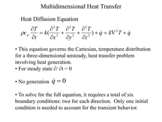
1. Multidimensional Heat Transfer
Heat Diffusion Equation
c
T
t
k
T
x
T
y
T
z
q k T q
p











   
( )  
2
2
2
2
2
2
2
• This equation governs the Cartesian, temperature distribution
for a three-dimensional unsteady, heat transfer problem
involving heat generation.
• For steady state / t = 0
• No generation
• To solve for the full equation, it requires a total of six
boundary conditions: two for each direction. Only one initial
condition is needed to account for the transient behavior.

q  0

2. Two-D, Steady State Case
For a 2 - D, steady state situation, the heat equation is simplified to
it needs two boundary conditions in each direction.
2 2






T
x
T
y
2 2
0,
There are three approaches to solve this equation:
• Numerical Method: Finite difference or finite element schemes,
usually will be solved using computers.
• Graphical Method: Limited use. However, the conduction
shape factor concept derived under this concept can be useful for
specific configurations.
• Analytical Method: The mathematical equation can be solved
using techniques like the method of separation of variables.
(review Engr. Math II)

3. Conduction Shape Factor
This approach applied to 2-D conduction involving two
isothermal surfaces, with all other surfaces being adiabatic. The
heat transfer from one surface (at a temperature T1) to the other
surface (at T2) can be expressed as: q=Sk(T1-T2) where k is the
thermal conductivity of the solid and S is the conduction shape
factor.
• The shape factor can be related to the thermal resistance:
q=Sk(T1-T2)=(T1-T2)/(1/kS)= (T1-T2)/Rt
where Rt = 1/(kS)
• 1-D heat transfer can use shape factor also. Ex: heat transfer
inside a plane wall of thickness L is q=kA(DT/L), S=A/L
• Common shape factors for selected configurations can be
found in Table 17-5

4. Example
An Alaska oil pipe line is buried in the earth at a depth of 1 m.
The horizontal pipe is a thin-walled of outside diameter of 50
cm. The pipe is very long and the averaged temperature of the
oil is 100C and the ground soil temperature is at -20 C
(ksoil=0.5W/m.K), estimate the heat loss per unit length of pipe.
z=1 m
T2
T1
From Table 17-5, case 1.
L>>D, z>3D/2
S
L
z D
q kS T T
W
  
   

2
4
2 1
4 0 5
3 02
0 5 3 02 100 20
1812
1 2
 
ln( / )
( )
ln( / . )
.
( ) ( . )( . )( )
. ( ) heat loss for every meter of pipe

5. Example (cont.)
T
C
m p

T
C
m p

If the mass flow rate of the oil is 2 kg/s and the specific heat of the oil
is 2 kJ/kg.K, determine the temperature change in 1 m of pipe length.
q mC T T
q
mC
C
P
P
    
 ,

.
*
. ( )
D D
1812
2000 2
0 045
Therefore, the total temperature variation can be significant if the pipe
is very long. For example, 45C for every 1 km of pipe length.
• Heating might be needed to prevent the oil from freezing up.
• The heat transfer can not be considered constant for a long pipe
Ground at -20C
Heat transfer to the ground (q)
Length dx
)
( dT
T
C
m p 


6. Example (cont.)
Heat Transfer at section with a temperature T(x)
q =
2 k(dx)
ln(4z / D)
Energy balance: mC
integrate
at inlet x = 0, T(0) = 100 C, C = 120
T(x) = -20 +120
P

( ) . ( )( )
  ( )
 . ( ) , . ,
( ) ,
.
.
T T dx
T q mC T dT
mC
dT
dx
T
dT
T
dx
T x Ce
e
P
P
x
x
  
  
  

 
   


20 151 20
151 20 0
20
0 000378
20 0 000378
0 000378
0 1000 2000 3000 4000 5000
50
0
50
100
T( )
x
x
• Temperature drops exponentially
from the initial temp. of 100C
• It reaches 0C at x=4740 m,
therefore, reheating is required
every 4.7 km.