1. Taxicab Modeling
Carl Bucella, Kelsey Harrington, Corey Marsh
Novemeber 17th, 2013
Abstract
To address the need for improved taxi services in the Town of Mythical, we have
developed a model that uses a minimum-weight pairing algorithm and discrete event
simulation. The minimum-weight pairing algorithm matches available cabs with in-
coming customer orders so as to minimize customer wait times. The discrete event
simulation generates Poisson distributed orders and probabilistically defined starting
and ending locations dependent on the time of day. After running multiple simulation,
we were able to determine an estimated upper and lower bound for the number of cabs
needed to ensure that the average customer wait time was under 15 minutes and that
less than 10% of customers had to wait more than 25 minutes. Our upper bound esti-
mate is based on the assumption that the distance between two points was calculated
using right-angle distance, i.e. d = |x2 − x1| + |y2 − y1|. Our lower bound estimate
uses the Euclidean distance between two points, i.e. it assumes there is a straight line
path between point a and point b. A visual validation of the results is performed by
graphing the average customer wait time and the percentage of customers who wait
longer than 25 minutes as a function of the number of cabs in operation. We develop
our model further by implementing both fixed and variable pricing functions. In order
to maintain the current levels of revenues for local taxi companies as determined by
the fixed pricing structure, a variable cost of $X per mile is suggested. Finally, we
consider the effect of an increase or decrease in the market share of unlicensed cab
companies. Our results determine that stricter regulations against unlicensed compa-
nies would decrease the average wait time for taxi customers in Mythical, so we are in
favor of greatly strengthening the regulations against unlicensed cab companies.
1

2. Contents
1 Problem Statement 3
2 Problem Analysis and Possible Models 3
2.1 Definition of Parameters . . . . . . . . . . . . . . . . . . . . . . . . . . . 3
2.2 Modeling Orders Arrivals . . . . . . . . . . . . . . . . . . . . . . . . . . 5
2.2.1 Uniform Distribution . . . . . . . . . . . . . . . . . . . . . . . . . 5
2.2.2 Poisson Distribution . . . . . . . . . . . . . . . . . . . . . . . . . . 5
2.3 Modeling Call Pick-Up and Drop-Off Locations . . . . . . . . . . . . 6
2.4 Modeling Travel Time . . . . . . . . . . . . . . . . . . . . . . . . . . . . 7
2.5 Modeling Cab Responses to Calls . . . . . . . . . . . . . . . . . . . . . 8
2.5.1 Minimal Weight Matching . . . . . . . . . . . . . . . . . . . . . . 8
2.5.2 Minimal Weight Spanning Tree with Priority . . . . . . . . . 8
2.6 Modeling Pricing . . . . . . . . . . . . . . . . . . . . . . . . . . . . . . . . 9
2.6.1 Prelimary Zone Pricing Analysis . . . . . . . . . . . . . . . . . . 10
2.6.2 Zone Pricing Simulation . . . . . . . . . . . . . . . . . . . . . . . 10
2.7 Modeling Market Share Differences . . . . . . . . . . . . . . . . . . . . 10
3 Results 11
3.1 Required Number of Taxicabs . . . . . . . . . . . . . . . . . . . . . . . 11
3.2 Pricing Analysis . . . . . . . . . . . . . . . . . . . . . . . . . . . . . . . . 13
3.2.1 Simulated Pricing Analysis . . . . . . . . . . . . . . . . . . . . . . . . 13
3.3 Market Share Results . . . . . . . . . . . . . . . . . . . . . . . . . . . . . 15
4 Strengths and Weaknesses of the Proposed Model 16
5 Robustness - Sensitivity of λ∗
16
6 Further Extensions and Considerations 18
7 Appendix 19
7.1 MATLAB code for Parts 1 and 2 . . . . . . . . . . . . . . . . . . . . . . 19
7.2 MATLAB code for Part 4 . . . . . . . . . . . . . . . . . . . . . . . . . . 36
2

3. 1 Problem Statement
Mythical city and county officials are interested in improving the quality and price of services
offered by local taxi companies. In order to do so, they have asked us to determine:
1. The total number of cabs needed to serve the ”Greater Mythical” area such that the
average customer is waiting for no more than 15 minutes and less than 10% of customers
are waiting for more than 25 minutes.
2. The value X that would cause taxicab revenues to be roughly the same as they are
now if the city switches to meter-based pricing where you pay a $2.50 flat rate and X
cents per mile. Currently the city has determined taxi ride prices based on originating
and terminating zones.
3. The impact on the average wait times and prices of non-regulated rides if the con-
glomerate, Mythical Dispatch, Inc. were to be splitup into 3 companies that operated
independently from each other. Mythical Dispatch, Inc. currently owns 2/3 of all cabs
officially licensed in the city.
4. The consequences of strengthening regulations against unlicensed companies, who cur-
rently contol about 1/7 of all cabs in the city.
Disclaimer: Upon reading the problem statement, we immediately noticed a similarity be-
tween the Town of Mythical and the Town of Ithaca. We base our assumptions and calcu-
lations heavily on the Town of Ithaca. However, we must stress that these similarities are
only a coincidence, and that our model was specifically designed for the fictional Town of
Mythical. Therefore, whenever we refer to information about the Town of Ithaca, we are
only doing so because it provides accurate background information for our model.
2 Problem Analysis and Possible Models
Our models focus on providing answers to the first, second, and fourth parts of the problem.
2.1 Definition of Parameters
In order to solve this problem, we made some simplifying assumptions:
1. The Town of Mythical has specific regions and points of interest. Based
on the problem statement, we know that the town of Mythical has a large college
(Mornell University), a small liberal arts college (Mythical College), an airport, a
mall, a downtown area, etc. In order to make our problem simpler, we based these
regions and points of interest off of the corresponding regions for the Town of Ithaca.
3

4. 2. The taxis travel at a constant velocity of 25 miles per hour. We estimated the
average miles per hour for roads in the Town of Ithaca to be around 40. Within the
City, the speed limit is 35 miles per hour, but in the surrounding areas the speed limit
can become as high as 65 miles per hour. The roads with higher speed limits are less
common, so we estimated the average speed limit to be closer to 40 miles per hour. In
order to account for traffic, traffic lights, stop signs, etc. we decided to set the average
speed to 25 miles per hour.
3. The Greater Mythical Area is approximately a 6.6832 by 5.1602 mile rect-
angle. We assumed that the Town of Ithaca is similar in size to the Town of Mythical.
Using a map image for the Town of Ithaca, [1], as well as the scale image for the map,
we processed the two images in MATLAB to determine the size of Ithaca and in turn,
Mythical.
4. The expected number of orders is a function of time. The idea that customer
orders are time dependent is based on empirical evidence gathered as a result of research
into the taxicab system in Boston, [2]. Although we were unable to find specific data
on the expected number of orders at each point in time, we were able to estimate these
values using our own personal experience. For example, it is likely that a taxi company
receives far less customer orders between 2 AM and 6 AM than it does between 8 PM
and 11 PM. Later, we discuss using a Poisson distribution to determine the number of
orders per minute. We designed our values of λ(t) to reflect our prior knowledge and
experience.
5. There are specific probabilities for the starting and ending region of a trip
based on the time of day. We know that based on the time of day, people are
more likely to travel from certain places to others. We also know that the probability
of ending in one region is likely conditional on the region the trip started in. The
numbers we came up for these probabilities are based on various factors:
• There are no flights in and out of the airport between 2AM and 5 AM, so the
probability of getting a order from or to the airport during these hours is 0, [3].
• The mall is closed from 10 PM to 8 AM, so the probability of getting an order to
or from the mall during these hours is 0, [4].
• People travel to and from downtown more frequently between the hours of 11 PM
to 2 AM, so the probability of receiving calls from and to these areas is greater
during that time period.
• If you are starting your order from a random location in the Town of Mythical,
then you are likely traveling to one of the main regions (Airport, Mall, Mornell,
etc.), so the probability of going to these areas is higher.
4

5. • If you are starting your order from one of these main regions (Airport, Mall,
Mornell, etc.), it is likely that you do not have a car and are therefore a student,
so you have a higher probability of traveling to Mornell or Mythical College.
A lot of thought went into determining these probabilities. We combined the in-
formation about taxi cab transportation in Boston, [2], with our own knowlege and
experience, to determine the values of these probabilites.
2.2 Modeling Orders Arrivals
2.2.1 Uniform Distribution
In our original model, we modeled order arrival times as uniform distribution over a 24-hour
day. For each iteration of our algorithm, which corresponds to a one-minute interval in real
time, we generated a random number uniformly distributed between 0 and 1. We checked if
that random number was less than a certain value c, where c ∈ [0, 1], to determine whether a
customer placed an order in that time interval. The value of c corresponded to the expected
number of orders, which we set to 0.3 and 1.0 in trial runs but later determined would likely
be somewhere between these values, approximately 0.8.
Although the choice of uniformly distributed order arrivals helped to simplify the imple-
mentation of our model, the assumption fails to account for changes in customer demand
dependent on the time of day. Furthermore, the uniform assumption restricted the number
of possible orders that could be placed in a minute to zero and one. In a town with a strong
college presence such as Mythical, it is very likely that multiple orders will be placed in a
given minute during peak hours, especially when there is an event, such as a concert. It is
assumed that many college students do not have cars and it is estimated that they make up
a large portion of taxicab customers in Mythical.
2.2.2 Poisson Distribution
Based on our research, we settled on a Poisson distribution for modeling the order arrivals.
Arrival times are often modeled using the Poisson distribution in other applications, and
because our algorithm is a discrete-event simulation with a variable λ parameter, this distri-
bution works well. The distribution function for a Poisson random variable is given below:
f(k; λ) = P(X = k) =
λ(t)k
e−λ(t)
k!
(1)
This choice also allows us to vary λ, corresponding to the expected number of orders, as
a function of time. As we discussed above, the expected number of orders per minute is
dependent upon the time of day. Our model implements a piece-wise function for λ, given
below. The function shows that the taxicab companys peak hours are between 8 PM and
5

6. midnight, and that the lowest frequency of orders can be expected to occur between 2 AM
and 6 AM. Our choices for these values are our best estimates based on observations of
taxicab use in a town very similar to Mythical. Our λ values are based on the value of λ∗
,
which is the expected number of calls per minute between 6 AM - 4 PM (midday). We used
λ∗
to calculate the other values of λ, as can be seen below, and varied λ∗
to see how this
would change our output.
E(X) = λ(t) =



1.2λ∗
if t is between 12AM-2AM
0.2λ∗
if t is between 2AM-6AM
1.0λ∗
if t is between 6AM-4PM
1.2λ∗
if t is between 4PM-8PM
1.6λ∗
if t is between 8PM-12AM
2.3 Modeling Call Pick-Up and Drop-Off Locations
We originially selected random x and y values that were in the ”Greater Mythical Region”.
Later we decided to select the trip starting and ending locations based on time of day and
points of interest, as is alluded to in our definition of parameters. Most of the orders will
originate or end in the ”City of Mythical” and/or a point of interest (Airport, Mall, Mornell,
etc.). Outside of the city is assumed to be predominantly agricultural with fewer roads and
the people living there are assumed to own cars therefore, fewer orders would originate from
or go to these regions. We assigned different probabilities, that varied with time of day, that
an order is placed from a region and that an order will end in another region (conditional
on the region the order was placed in). The main regions that we consider are:
1. The Mythical-Dompkins Airport - considered as Zone 7
2. Mythical Mall - considered as Zone 8
3. Mornell University - Zones 5 and 6
4. Mythical College - considered as Zone 9
5. Downtown Mythical - Zones 3 and 4
6. The parts of the City of Mythical that have not previously been considered - Zones 1
and 2
7. The parts of the Town of Mythical that have not previously been considered - consid-
ered as Zone 10
Zones 1 through 6 correspond to the pricing zones, [5], and are used in the pricing section.
Once the starting and ending regions were determined, the starting and ending points were
randomly selected from within the rectangular approximations to each zone displayed on the
following page.
6

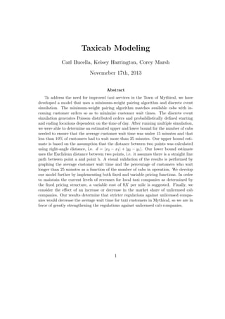
7. Figure 1: Map of ”Greater Mythical Area” with Zones
2.4 Modeling Travel Time
In our model, we have two different options for calculating the travel time between two points.
Our initial simplification was to simply use the Euclidean distance formula to calculate the
distance between two points. In order to find the time it takes to travel this distance, we
divide this distance by our assumed velocity.
d = (x1 − x2)2 + (y1 − y2)2 (2)
While this distance greatly simplifies our model, we realize that it is very unrealistic to
assume that you can get between any two points in a straight line considering that roads
rarely allow this. Using this formula for distance therefore, gives us a lower bound for our
simulation results.
In order to combat this issue, we use the following distance formula to find the upper
7

8. bound. Which is the sum of the total x distance and y distance traveled between two points.
d = |x2 − x1| + |y2 − y1| (3)
This formula represents the distance the trip would be if you could only travel at right angles
between the two points. We later refer to this as the right angle distance between the two
points.
While we did not have time to make a more detailed distance function based off of roads
and speed limits, the use of these two functions to find an upper and lower bound for the
travel time makes our model more robust than simply choosing one.
2.5 Modeling Cab Responses to Calls
2.5.1 Minimal Weight Matching
In order to fill these orders, we need to find a matching between the list of available cabs
and the list of orders at each time step. If there are no available cabs or no new orders at
time t, we do not perform a matching and increment t. We repeat this process until we
have at least one available cab and new order. At this point, we call fillOrders to find the
matching between the orders and cabs. fillOrders uses an adaptation of Kruskals algorithm
to find the minimal distance pairing between the two sets. In order to do so, fillOrders stores
the wait time from every cab A to every order B. This list is then sorted by the distances
so that the smallest distance is at the top of the list. Then, fillOrders considers the edges
in increasing order; if the cab for the edge is available, and the order is still unfilled, we
accept this edge. We repeat this process, and ignore any edges where the cab and order have
already been used/filled. Once we have filled all the orders, or used all possible cabs, the
process is finished.
Using the list of filled orders, we update the list of cabs with their final locations, as well
as the time for which they will be unavailable. In order to calculate the unavailable time,
we add the wait time to the time of the trip. We have already modeled the start and end
positions of each order, so this information is easily calculated from our list of orders. We
create a vector that contains the wait times for each filled order during the current time step.
At the end of fillOrders, we return this vector and concatenate it with the vector containing
data for the previous wait times. At the end of the simulation, we are left with a vector of
wait times for each order placed, which we analyze to determine the result of the simulation.
2.5.2 Minimal Weight Spanning Tree with Priority
One issue with the method above is that the orders are filled only based on the distance
between them and the nearest available cabs. This could cause orders far away from all
available cabs to remain unfilled for long periods of time, and we did not feel that this
8

9. coincides with how a cab company would typically operate. In order to fix this problem, we
treat the list of orders as a queue. A queue operates by the first-in-first-out (FIFO) property,
so the oldest orders placed are considered first before any new orders. If there are two orders
that were placed at the same time, we always consider them together, to prevent favoring
the order that was stored in the list first. The orders are then processed in the same way as
before, but only the oldest orders are considered by the matching algorithm.
2.6 Modeling Pricing
We based our model pricing off of the following map of each zone and the corresponding
zone-to-zone prices listed in the matrix below, [5].
Figure 2: Map of Zones
Figure 3: Zone Pricing
9

10. 1 2 3 4 5 6
1 - 1.83 1.89 1.73 3.1 2.6
2 1.83 - 1.88 1.19 2.75 2.24
3 1.89 1.88 - 0.87 1.62 1.67
4 1.73 1.19 0.87 - 1.71 1.21
5 3.1 2.75 1.62 1.71 - 1.2
6 2.6 2.24 1.67 1.21 1.2 -
Table 1: Distance between Zone Centers (mi)
2.6.1 Prelimary Zone Pricing Analysis
To start our zone pricing analysis we calculated the distance from the center of each zone
to the center of each other zone, using MapQuest, [6]. Our results are listed in the table
above. We then subtracted $2.50, the base price for a cab ride, from the zone prices depicted
in Figure 3 and divided the remaining price by the distance between the zone centers. We
then averaged these prices to get the average price per mile that would need to be charged
for the metered pricing to be roughly equilivalent to the fixed zone pricing.
2.6.2 Zone Pricing Simulation
The problem asked us to leave the revenues of cab companies, rather than prices per trip,
relatively the same as they are now. Therefore, in order to more accurately compare the
difference in revenue between a fixed price plan and a variable price plan (for orders placed
within the city), we calculate and store the two prices for each trip. From the order infor-
mation, we know the two zones that the order is traveling between, as well as the x and y
coordinates of the start and end points. Using the zones along with the zone pricing map,
[5], we calculate the fixed price of the order. Similarly, we use the x and y coordinates to
calculate the variable price for the trip. Both of these values are returned by fillOrders for
the orders filled in the current time step. Like wait time, we concatenate this new vector
with the vector holding the previous prices of orders. At the end of the simulation, we are
left with a 2 by p matrix, where P(1,i) is the fixed price for order i, and P(2,i) is the variable
price for the same order.
2.7 Modeling Market Share Differences
In order to solve part 4 of the problem statement, we needed to set up a simulation in
which there are two distinct cab companies operating within the City of Mythical. The first
company is considered to be Mythical Dispatch, the conglomerate of 3 companies, while
10

11. Company 2 is assumed to be the group of non-regulated taxicab companies. Because of the
way our code was written, it was simple to complete this by performing the following steps:
• First, we defined the total number of cabs in mythical (n) and the market share of
company 2 (m).
• Second, we created separate data structures for Company 2 to hold the data for their
cabs, orders, available cabs, wait times, and prices.
Then, we modified orders so that if a person is traveling within the City of Mythical, they
have probability m of calling Company 2. This assumption follows directly from the definition
of market share. Using a uniform distribution, we determine which company should get a
specific order, and then return two lists of orders, one for each company. We then call
fillOrders for each company, using the appropriate data structures for each. At the end of
the simulation, we are left with a list of wait times and prices for each company, which we
then analyze to determine our results.
3 Results
3.1 Required Number of Taxicabs
After using our model to simulate a 24-hour day over 25 trials, we were able to determine
the total number of cabs needed to serve the ”Greater Mythical” area. The graphs on the
following page show the average wait time and percent of people who wait longer than 25
minutes as a function of the number of cabs operating.
The figures show that the average wait time decreases as the number of taxis increases,
which is to be expected. The rate of decrease appears to be consistent with logistic decay
since the average wait time decreases less as the number of taxis increases. Therefore,
deploying more cabs than is necessary to meet the city’s goals does not result in an equivalent
increase in productivity. We ran our simulation using both the Euclidean distance, which
serves as a lower bound for the number of cabs necessary, and using the right angle distance,
which serves as an upper bound for the number of cabs. Our lower and upper bound estimates
for the number of cabs necessary to meet the citys goals are 11 and 14 cabs respectively.
11

12. Figure 4: Average Wait Time and % of Wait Times Over 25 min for Euclidean Distance
Figure 5: Average Wait Time and % of Wait Times Over 25 min for Right Angle Distance
12

13. 1 2 3 4 5 6
1 - 1.42 1.38 1.50 1.00 1.19
2 1.42 - 1.38 2.18 1.13 1.38
3 1.38 1.38 - 2.99 1.60 1.56
4 1.50 2.18 0.87 - 1.52 2.15
5 1.00 1.13 1.62 1.52 - 2.17
6 1.19 1.38 1.67 2.15 2.17 -
Table 2: Distance between Zone Centers (mi)
3.2 Pricing Analysis
The results of our preliminary pricing analysis are shown above. We found that the average
price per mile from one zone center to another should be approximately $1.64 (average of
the values depicted). This is the price per mile needed to keep the trip from one zone center
to another roughly equal to what it is currently.
3.2.1 Simulated Pricing Analysis
The results of our simulated pricing analysis using 15 cabs and λ∗
= 0.8 are depicted on the
following page. We varied price per mile from $0.50 to $3.00 by $0.10. We ran the simulation
for only 5 days for each price per mile and calculated the daily revenue difference for each
of these days. This was believed to be sufficient since there are several orders per day and
that averaging the daily revenue difference over more days would produce a similar result.
Then we averaged these revenue differences to get the average daily price difference for each
price per mile. We found that the price of $2.00 per mile minimized the difference between
the average daily revenue when it is assumed you can only travel in right angles. We found
that the price of $2.50 per mile minimized the difference between the average daily revenue
when it is assumed you can travel straight to your final destination, calculated using the
Euclidean distance formula. This makes sense because using the right angle distance causes
trips to be longer than when you travel straight there causing the price per mile of the right
angle distance to be less if we are trying to keep the overall revenue the same. These values
are slightly larger than the ones found by our prelimary analysis but still relatively close
and we believe that these are more accurate since they take more parameters into account.
Therefore, we conclude that the average price per mile should be $2.25 if we want to switch
to metered pricing but leave the revenues of taxicab companies roughly the same as they are
currently. The advantage to switching to meters is that a cab company could make more
money if they are traveling further into a zone than before however, a disadvantage is that
13

14. they could make less money if they are just barely entering a new zone. The cab driver’s
hapiness likely depends on whether they are making more or less money and the city and
county officials likely want to keep the cab drivers happy.
Figure 6: Right Angle Distance
Figure 7: Euclidean Distance
14

15. 3.3 Market Share Results
In order to see the effect of market share on wait time, we set the value of n to 20 and λ∗
to
1.2. We increased the number of cabs and the average number of orders per minute so, it is
easier to represent a smaller percentage of the market share by Company 2. Then, we ran
MythicalCabs2 for multiple trials for each value of m (market share). This resulted in the
following graphs:
Figure 8: Average Wait Time for Variable Market Shares
Figure 9: % of Wait Times over 25 min for Variable Market Shares
15

16. As you can see, adding a second cab company with a market share of 1/7 drastically
increases the average wait time of all customers. From these results, we can easily make a
conclusion about the effect of reducing the market share of Company 2. If you reduce the
market share of Company 2, the average wait times for everyone will decrease. Therefore,
we are in favor of stricter regulations on the unlicensed cab companies operating within the
city.
4 Strengths and Weaknesses of the Proposed Model
The main strength of our model is its adaptability. This is partly due to the nature of our
model, and partly due to the way we broke down our code into functions. For example,
writing separate functions for generating orders and filling orders made it very easy to add
a second cab company and monitor the effect of its market share. Not only was our code
compartmentalized well, but the parameters that determine the model are easily adjustable,
so it was very easy for us to run the simulation over many trials while varying certain
parameters. This allowed us to easily perform sensitivity tests on our data, which will be
discussed in the Sensitivity of λ∗
section.
Our model has one main weakness, which is in how the travel time is calculated. While
we use the two different distance formulas to provide an upper and lower bound for our
results, it is obvious that our model would be more accurate if we forced cabs to stay on a
predetermined set of roads, with designated speed limits for each road. In the city, where
the roads are more densely packed, this simplification does not affect our model too much.
However, in the town of Ithaca, where roads are more spread out, this simplification will
cause more inaccuracy. The distance traveled on these roads could vary from our distance
calculations, and our average velocity is probably lower than the actual average velocity
when traveling in the town. There is a way to remove this weakness, which will be discussed
in the Further Extensions and Considerations section.
5 Robustness - Sensitivity of λ∗
While we used background data to determine our value for λ∗
, we wanted to see how changing
the value of λ∗
by a small amount affected the average wait time based on a fixed number
of cabs. In order to do so, we ran multiple trials where we varied λ∗
from 0 to 2 while
keeping the number of cabs constant. Running this experiment helped us to validate our
results in the following way: we noticed that as λ∗
increases, the average wait time grows
logistically, which we expect because after a certain point, the wait times are already so large
that increasing λ∗
does not have much of an effect.
16

17. Figure 10: Average Wait Time for Variable Values of λ∗
Figure 11: % of Wait Times over 25 min for Variable Values of λ∗
We noticed from earlier experiments that for every λ∗
, there is a value for n (number of
cabs) which is essentially a ”tipping point”. This tipping point represents the number of
cabs for which the company is able to keep up with the orders it receives. For n less than
this tipping point, the cab company will not be able to keep up with the orders. As the
number of unfilled orders increase, the wait times grow exponentially. By keeping n fixed and
running the simulation while varying λ∗
, this could tell a company with n cabs the average
orders per minute that they would be capable of serving. While we did not intend to solve
17

18. this problem, it is an interesting result nonetheless.
6 Further Extensions and Considerations
As we discussed in our Strengths and Weaknesses section, our model has one main weakness:
the estimation of travel time and distance. There is a simple way to solve this, but it requires
a lot of time to gather the appropriate data and write the algorithm. This is how we would
approach this problem if we had time:
First, we would need to collect data for the intersections and roads of Mythical. We
would create a graph, with nodes representing the various intersections throughout Mythical
and edges representing the roads between the intersections. The weight of each edge would
be the time required to travel the edge, which is the distance of the edge divided by the
speed limit of the edge. After determining the starting and ending points of a route, we
would use Dijkstras algorithm to find the shortest weighted path from point A to point B,
and return the total time and distance of the path.
To take this method even further, we could also return the number of nodes on the path
and use it to estimate the time waited at lights. For example, we could assume that there
is some probability (p) that a node N has a traffic light. So, for each node passed, we could
check if there was a traffic light at that node using a uniform distribution. If there is a traffic
light, we could model the wait time at the light on a normal distribution, where wait times
less than or equal to zero mean the light is green when you pass it. If we added the wait
time from each node to the wait time of the trip, the accuracy of our travel time between
two points would increase dramatically.
18

19. 7 Appendix
7.1 MATLAB code for Parts 1 and 2
%The following script runs the simulation for N trials on each value of n,
%and graphs the results
close all
N = 25;
upper_bound = true;
n_s = 5; %Starting number of cabs
n = 15; % iterate over n cabs per trials
x = []; % x-axis vector
avgwait = []; % average wait time
perover25 = []; % percentage wait times greater than 25min
sum_perover25 = zeros(1,n);
sum_avgwait = zeros(1,n);
X = 2; %Price per mile
for k = 1:N
perover25 = [];
x = [];
avgwait = [];
for i=n_s:n+n_s-1
x=[x i];
[wait,price] = MythicalCabs(i,X,upper_bound);
avgwait=[avgwait, mean(wait)];
over25=0;
for j=1:length(wait)
if wait(j)>25
over25=over25+1;
end
end
over25=100*over25/length(wait);
perover25=[perover25 over25];
end
sum_avgwait = sum_avgwait + avgwait;
avg_avgwait = sum_avgwait/N;
19

20. sum_perover25 = sum_perover25 + perover25;
avg_perover25 = sum_perover25/N;
end
figure
bar(x,avg_avgwait);
xlabel(’Number of Taxis’);
ylabel(’Average Wait Time’);
figure
bar(x,avg_perover25);
hold on
line(’XData’, [0 n+5], ’YData’, [10 10], ’LineStyle’, ’-’, ...
’LineWidth’, 2, ’Color’,’r’)
xlabel(’Number of Taxis’);
ylabel(’% of Wait Times Greater Than 25min’);
function [M,I] = PricingGraph()
% Displays a graph of the average daily revenue difference based on price
% per mile
close all
r_diff=[];
xax=[];
for X=0.5:0.1:4 % set price values = 0.5,0.6,...,4.0
xax=[xax,X];
r_diffd=[];
for d=1:5
[W,P]=MythicalCabs(15,X,true);
% daily revenue difference
r_diffd=[r_diffd, sum(P(1,:))-sum(P(2,:))];
end
% calculate average revenue difference over 5 days
r_diff=[r_diff, mean(r_diffd)];
end
[M,I]=min(r_diff);
20

21. bar(xax,r_diff);
title(’Average Price Difference’);
xlabel(’Price ($/mi)’);
ylabel(’Average Price Difference’);
end
function [W,P] = MythicalCabs(n,X,bound_flag)
%The following script simulates the movement of cabs around the city of
%Mythical in order to determine the wait times of customers.
%If bound_flag is false, use the straight line distance between points
%to find the lower bound for the number of cabs.
%If bound_flag is true, use the right angle distance between two points
%to find the upper bound for the number of cabs.
t_stop = 24*60; %The length of the simulation in minutes
%The following array holds the information about the position of the cabs,
%as well as the remaining time that they are unavailable
C = zeros(n,3);
W = []; %This vector contains the wait times for all filled orders
O = []; %The initially empty vector of orders
P = [;];
%Fill in the array C with random starting positions, and a current time
%unavailable of 1
for i = 1:n
C(i,1) = rand(1)*5.6832;
C(i,2) = rand(1)*5.1602;
C(i,3) = 1;
end
%Main simulation loop
for t = 1:t_stop
C(:,3) = C(:,3)-1; %Each cab has one less minute until available
%Generate the list of new orders (O) for this time step, return as a
%vector of with width 5 (x1,y1,x2,y2,t)
%Concatenate this vector with the vector of remaining orders
21

22. new_O = orders(t);
O = [O ; new_O];
%The following vector is the list of indeces for available cabs for
%the current time step. If i is in A, then C(i) is available
A = [];
j = 1;
for i = 1:n
if C(i,3) <= 0 %If the cab is available
A(j) = i; %Store the index in a temp array T
j = j + 1; %Increment j
end
end
%Get the updated C and O vectors after filling orders during this time
%step. Also get the wait times for filling the orders.
if ~isempty(A) && ~isempty(O)
[C,O,temp_W,temp_P] = fillOrders(t,A,C,O,X,bound_flag);
P = [P temp_P];
W = [W temp_W]; %Add the new wait times to the current list
end
end
end
function O = orders(t)
current_hr = t/60; % converts t into hours
factor = [1.2, .2, 1.6]; % determines percent increase or decrease of opm
lambda = .8;
% this block of code varies the orders per minute based on
% the time of day i.e. hour 0 is midnight, 1 is 1 AM, 2 is 2 AM
% etc... so hour 24 corresponds to midnight of next day
if current_hr <= 2
% set prob of starting location being cornell or IC to be
% a higher probability.
% set prob of ending location being somewhere on either of those
22

23. % campuses to be high prob...ie most trips should be a short
% distance (downtown,cornell; downtown, ic; cornell, cornell; etc)
randOrder = poissrnd(factor(1)*lambda);
if randOrder <= 0 % if 0 orders this minute, set O to empty
O = [];
return; % if randOrder = 0, that means 0 orders in this minute so
% return to MythicalCabs and go to next time step
end
O = zeros(randOrder,7);
for i = 1:randOrder
position = location(t);
O(i,1) = position(1); % starting x-coord of order
O(i,2) = position(2); % starting y-coord
O(i,3) = position(3); % ending x-coord
O(i,4) = position(4); % ending y-coord;
O(i,5) = t; % time order placed (in mins)
O(i,6) = position(5); % beginning region of order
O(i,7) = position(6); % ending region of order
end
elseif current_hr <= 6
% Decrease orders per minute, i.e. there will be significantly
% less orders between 2 AM and 6 AM
randOrder = poissrnd(factor(2)*lambda);
if randOrder <= 0 % if 0 orders this minute, set O to empty
O = [];
return; % if randOrder = 0, that means 0 orders in this minute so
% return to MythicalCabs and go to next time step
end
O = zeros(randOrder,7);
for i = 1:randOrder
position = location(t);
23

24. O(i,1) = position(1);
O(i,2) = position(2);
O(i,3) = position(3);
O(i,4) = position(4);
O(i,5) = t;
O(i,6) = position(5);
O(i,7) = position(6);
end
elseif current_hr <= 16
% Orders per minute should be higher than 2 AM - 6 AM but lower
% than 4 PM to midnight
% prob of starting and ending location being the mall or airport
% should be much higher for this time interval
randOrder = poissrnd(lambda);
if randOrder <= 0 % if 0 orders this minute, set O to empty
O = [];
return; % if randOrder = 0, that means 0 orders in this minute so
% return to MythicalCabs and go to next time step
end
O = zeros(randOrder,7);
for i = 1:randOrder
position = location(t);
O(i,1) = position(1);
O(i,2) = position(2);
O(i,3) = position(3);
O(i,4) = position(4);
O(i,5) = t;
O(i,6) = position(5);
O(i,7) = position(6);
end
elseif current_hr <= 20
% Orders per minute should be higher than 6 AM - 4 PM but slightly
% lower than 8 PM - Midnight
% prob of starting and ending location being mall or airport
24

25. % should be lower than for the 6 AM - 4 PM time interval
randOrder = poissrnd(factor(1)*lambda);
if randOrder <= 0 % if 0 orders this minute, set O to empty
O = [];
return; % if randOrder = 0, that means 0 orders in this minute so
% return to MythicalCabs and go to next time step
end
O = zeros(randOrder,7);
for i = 1:randOrder
position = location(t);
O(i,1) = position(1);
O(i,2) = position(2);
O(i,3) = position(3);
O(i,4) = position(4);
O(i,5) = t;
O(i,6) = position(5);
O(i,7) = position(6);
end
elseif current_hr <=24
% Orders per minute should be highest for this time interval
% starting and ending locations probabilities should be higher
% for collegetown, IC, downtown, i.e. trips should be shorter
% (not as many cabs going to/coming from the mall)
randOrder = poissrnd(factor(3)*lambda);
if randOrder <= 0 % if 0 orders this minute, set O to empty
O = [];
return; % if randOrder = 0, that means 0 orders in this minute so
% return to MythicalCabs and go to next time step
end
O = zeros(randOrder,7);
for i = 1:randOrder
25

26. position = location(t);
O(i,1) = position(1);
O(i,2) = position(2);
O(i,3) = position(3);
O(i,4) = position(4);
O(i,5) = t;
O(i,6) = position(5);
O(i,7) = position(6);
end
end
end
function [rC,rO,W,P] = fillOrders(t,A,C,O,X,b_f)
%This function takes three lists: A - the vector of available cabs,
%C - the list of all cabs, and O - the list of orders. Using these
%lists, it finds the matching that minimizes the total distance
%travelled when fufiling as many orders in O as possible. It returns
%three lists: rC - the cab list, updated with new positions and times
%of unavailability, rO - the list of remaining orders, and W - the list
%of the wait times for each order.
rC = C;
rO = [];
T_O = O;
O = [];
T = [];
W = [];
P = [;];
k = 1;
%If there are less cabs than orders
if length(A) < length(T_O(:,1));
r = find(T_O(:,5) == k,1,’last’);
while isempty(r) || r < length(A)
k = k + 1;
r = find(T_O(:,5) == k,1,’last’);
end
latest_considered_order_time = k;
26

27. else
latest_considered_order_time = max(T_O(:,5));
end
k = 1;
for i = 1:length(T_O(:,1))
if T_O(i,5) <= latest_considered_order_time
O(k,:) = T_O(i,:);
k = k + 1;
else
break
end
end
k = 1;
for i = 1:length(A)
A_i = A(i);
for j = 1:length(O(:,1))
T(k,1) = A_i; %Index of the cab
T(k,2) = j; %Index of the order
T(k,3) = t - O(j,5); %Time waited since call
T(k,4) = travelTime(C(A_i,1),C(A_i,2),O(j,1),O(j,2),b_f);
k = k + 1;
end
end
%Sorts the travel time collumn of T and stores the ordering
[values,order] = sort(T(:,4));
%Re orders T based on the order of travel time
T = T(order,:);
%The number of orders that will be filled. If there are less cabs than
%available orders, this will equal the number of available cabs. If
%there are less orders than available cabs, it will equal the number of
%orders.
orders_to_fill = min(length(A),length(O(:,1)));
filled_orders = 0; %The number of filled orders
used_C = []; %The list of cabs that have been used so far
filled_O = []; %The list of orders that have been filled
27

28. %The matrix used to store the filled orders for processing later
F = zeros(orders_to_fill,4);
j = 1;
k = 1;
while filled_orders < orders_to_fill
%If the cab and order for the current edge are not already
%used/filled
a = find(used_C == T(j,1),1);
b = find(filled_O == T(j,2),1);
ins_flag = isempty(a) && isempty(b);
if ins_flag
F(k,:) = T(j,:); %Store the current edge data in F
k = k + 1; %Increment k
filled_orders = filled_orders + 1; %Increment filled_orders
used_C = [used_C T(j,1)]; %Add the current cab to the used list
filled_O = [filled_O T(j,2)]; %Add the current order to the filled l
end
j = j + 1;
end
for i = 1:length(F(:,1))
F_cab = F(i,1); %The cab used for order i
F_order = F(i,2); %The index of the order filled
W_time = F(i,3) + F(i,4);
[U_time,U_dist] = travelTime(O(F_order,1),O(F_order,2),O(F_order,3),...
O(F_order,4),b_f);
U_time = U_time + W_time;
if O(F_order,6) <= 6 && O(F_order,7) <= 6
[prices(1,1) , prices(2,1)] = pricing(U_dist,X,O(F_order,6),O(F_order,7));
P = [P prices];
end
rC(F_cab,1) = O(F_order,3); %Update the x coordinate
rC(F_cab,2) = O(F_order,4); %Update the y coordinate
rC(F_cab,3) = ceil(U_time); %Update the unavailable time
28

29. W = [W W_time];
end
k = 1;
for i = 1:length(T_O(:,1))
if isempty(find(filled_O == i,1))
rO(k,:) = T_O(i,:);
k = k + 1;
end
end
end
function [out] = location( t )
% Used to generate which location an order will be made at and will be
% headed to based on a given time and will return the starting and ending x
% and y values and zones
% region 1: airport
% region 2: mall
% region 3: Mornell University
% region 4: Mythical College
% region 5: downtown Mythical
% region 6: City of Mythical
% region 7: Town of Mythical
p=zeros(1,7); %probabilities of being in each region
pg=zeros(7,7); %probabilities given in each region
if t<2 % btwn 12am and 2am, mainly college students out
p(3)=.5;
p(4)=.2;
p(5)=.2;
p(6)=.05;
p(7)=.05;
pg(3,:)=p;
pg(4,:)=p;
pg(5,:)=p;
pg(6,:)=p;
pg(7,:)=p;
29

30. elseif t < 6 % btwn 2am and 6pm only random ppl out
p(3)=.2;
p(4)=.2;
p(5)=.2;
p(6)=.2;
p(7)=.2;
pg(3,:)=p;
pg(4,:)=p;
pg(5,:)=p;
pg(6,:)=p;
pg(7,:)=p;
elseif t < 10 % btwn 6-10am, airport opens
p(1)=.3;
p(5)=.25;
p(6)=.25;
p(7)=.2;
pg(1,:)=[0,0,0,0,.35,.35,.3];
pg(5,:)=[.4,0,0,0,.25,.25,.1];
pg(6,:)=[.4,0,0,0,.25,.25,.1];
pg(7,:)=[.4,0,0,0,.25,.25,.1];
elseif t < 5 % btwn 10am-5pm, students in class
p(1)=.2;
p(2)=.2;
p(5)=.2;
p(6)=.2;
p(7)=.2;
pg(1,:)=[0,0,0,0,.4,.3,.3];
pg(2,:)=[0,0,0,0,.4,.3,.3];
pg(5,:)=[.3,.3,0,0,.2,.1,.1];
pg(6,:)=[.3,.3,0,0,.2,.1,.1];
pg(7,:)=[.3,.3,0,0,.2,.1,.1];
elseif t < 9 % btwn 5-9pm, students out of class
p(1)=.2;
p(2)=.2;
p(3)=.2;
p(4)=.1;
p(5)=.2;
p(6)=.05;
p(7)=.05;
pg(1,:)=[0,0,.3,.2,.3,.1,.1];
30

31. pg(2,:)=[0,0,.3,.2,.3,.1,.1];
pg(3,:)=[.3,.3,.1,0,.2,.05,.05];
pg(4,:)=[.3,.3,0,1,.2,.05,.05];
pg(5,:)=[.3,.3,.15,.05,.1,.05,.05];
pg(6,:)=[.3,.3,.15,.05,.1,.05,.05];
pg(7,:)=[.3,.3,.15,.05,.1,.05,.05];
elseif t<11 % btwn 9-11pm
p(1)=.2;
p(3)=.3;
p(4)=.1;
p(5)=.3;
p(6)=.05;
p(7)=.05;
pg(1,:)=[0,0,.4,.2,.2,.1,.1];
pg(3,:)=[.1,0,.4,.2,.2,.05,.05];
pg(4,:)=[.1,0,.4,.2,.2,.05,.05];
pg(5,:)=[.1,0,.4,.2,.2,.05,.05];
pg(6,:)=[.1,0,.4,.2,.2,.05,.05];
pg(7,:)=[.1,0,.4,.2,.2,.05,.05];
else % after 11pm, mainly college students out
p(3)=.5;
p(4)=.2;
p(5)=.2;
p(6)=.05;
p(7)=.05;
pg(3,:)=[0,0,.4,.2,.2,.1,.1];
pg(4,:)=[0,0,.4,.2,.2,.1,.1];
pg(5,:)=[0,0,.4,.2,.2,.1,.1];
pg(6,:)=[0,0,.4,.2,.2,.1,.1];
pg(7,:)=[0,0,.4,.2,.2,.1,.1];
end
r1=path(p);
r2=path(pg(r1,:));
[x1,y1,z1]=getXYZone(r1);
[x2,y2,z2]=getXYZone(r2);
out=[x1,y1,x2,y2,z1,z2];
end
31

32. %Helper function that determines the region based on a list of probabilities pp
function [loc]=path(pp)
rr=rand();
for i=1:length(pp)
if rr<=pp(i)
loc=i;
break
else
pp(i+1)=pp(i)+pp(i+1); % cummulates probabilities
end
end
end
function [x,y,z] = getXYZone(r)
% Calculates a random x and y value within a given region and returns that
% x and y values and the pricing zone, z, that this point lies in
scale=70.7342; % pixels per mi
if r==1 % airport - zone 7
x=364;
y=0;
z=7;
elseif r==2 % mall - zone 8
x=279;
y=0;
z=8;
elseif r==3 % Mornell
rndd=rand();
if rndd<.5 % zone 6
x=51*rand()+266;
if x<281
y=33*rand()+159;
else
y=49*rand()+159;
end
z=6;
else % zone 5
x=53*rand()+264;
32

33. y=72*rand()+87;
z=5;
end
elseif r==4 % Mythical College - zone 10
x=15*rand()+201;
y=34*rand()+252;
z=10;
elseif r==5 % downtown Mythical
rndd=rand();
if rndd<.5 % zone 4
y=49*rand()+159;
if y>192
x=75*rand()+206;
else
x=60*rand()+206;
end
z=4;
else % zone 3
y=72*rand()+87;
x=58*rand()+206;
z=3;
end
elseif r==6 % City of Mythical
rndd=rand();
if rndd<.5 % zone 1
y=119*rand()+40;
if y<87
x=68*rand()+168;
else
x=61*rand()+145;
end
z=1;
else % zone 2
x=61*rand()+145;
if x<161
y=50*rand()+159;
else
y=77*rand()+159;
end
33

34. z=2;
end
elseif r==7 % Town of Mythical - zone 9
rndd=rand();
if rndd<.4
x=145*rand();
y=365*rand();
elseif rndd<.7
k=0;
while k==0
x=157*rand()+145;
y=157*rand()+208;
if x<161 || x>206 || y>236
k=1;
end
end
elseif rndd<.9
x=85*rand()+317;
y=365*rand();
else
x=81*rand()+236;
y=87*rand();
end
z=9;
end
x=x/scale;
y=y/scale;
end
function [t,d] = travelTime(x1,y1,x2,y2,b_f)
%This function calculates the time it takes to travel between two
%points. Eventually, we can update this to be more accurate.
v = 25/60; %Velocity
X = [x1 y1 ; x2 y2];
if b_f
34

35. d = abs(x2-x1) + abs(y2-y1);
else
d = pdist(X,’euclidean’);
end
t = d/v;
end
function [p_fixed,p_variable] = pricing(d,mile_price,z1,z2)
%This function returns two prices for a cab trip. The first method uses
%the coordinates of the start and end point to find the distance
PF = [4.6 5.1 5.1 5.1 5.6 5.6 10 10 15 15.5;
5.1 4.6 5.1 5.1 5.6 5.6 12 12 15 15.5;
5.1 5.1 4.6 5.1 5.1 5.1 16 11.5 13 9.5;
5.1 5.1 5.1 4.6 5.1 5.1 16 11.5 13 9.5;
5.6 5.6 5.1 5.1 4.6 5.1 16 11.5 13 10.5;
5.6 5.6 5.1 5.1 5.1 4.6 16 11.5 13 10.5;
10 12 16 16 16 16 0 16 18 18;
10 12 11.5 11.5 11.5 11.5 0 16 18 15;
15 15 13 13 13 13 18 18 13 15;
15.5 15.5 9.5 9.5 10.5 10.5 18 15 15 5];
p_variable = 2.5 + d*mile_price;
p_fixed = PF(z1,z2);
end
35

36. 7.2 MATLAB code for Part 4
%Graphs the average wait time based on the market share of the two
%companies.
n = 20; %# of cabs
N = 50; %# of trials
lambda = 1.2;
upper_bound = false; %false denotes euclidean distance
x = []; % x-axis vector
avgwait = []; % average wait time
perover25 = []; % percentage wait times greater than 25min
sum_perover25 = zeros(1,21);
sum_avgwait = zeros(1,21);
X = 2; %Price per mile
for k = 1:N
perover25 = [];
x = [];
avgwait = [];
for i=1:21
x=[x i*.025-.025];
[W1,W2,P1,P2] = MythicalCabs2(i,X,upper_bound,i*.025,lambda);
wait = W1;
avgwait=[avgwait, mean(wait)];
over25=0;
for j=1:length(wait)
if wait(j)>25
over25=over25+1;
end
end
over25=100*over25/length(wait);
perover25=[perover25 over25];
end
sum_avgwait = sum_avgwait + avgwait;
avg_avgwait = sum_avgwait/N;
36

37. sum_perover25 = sum_perover25 + perover25;
avg_perover25 = sum_perover25/N;
end
figure
bar(x,avg_avgwait);
title(’Average Wait vs. Market Share of Company 2’);
xlabel(’Market Share’);
ylabel(’Average Wait Time’);
line(’XData’, [0 .5], ’YData’, [15 15], ’LineStyle’, ’-’, ...
’LineWidth’, 2, ’Color’,’r’)
axis tight
figure
bar(x,avg_perover25);
hold on
line(’XData’, [0 .5], ’YData’, [10 10], ’LineStyle’, ’-’, ...
’LineWidth’, 2, ’Color’,’r’)
xlabel(’Market Share’);
ylabel(’% of Wait Times Greater Than 25min’);
title(’% of Wait Times Greater Than 25min vs. Market Share of Company 2’);
axis tight
function [W1,W2,P1,P2] = MythicalCabs2(n,X,bound_flag,market_share,lambda)
%The following script simulates the movement of cabs around the city of
%Mythical in order to determine the wait times of customers.
%If bound_flag is false, use the straight line distance between points
%to find the lower bound for the number of cabs.
%If bound_flag is true, use the right angle distance between two points
%to find the upper bound for the number of cabs.
t_stop = 24*60; %The length of the simulation in minutes
%The following array holds the information about the position of the cabs,
%as well as the remaining time that they are unavailable (for companies
%one and two)
C1 = zeros(n-ceil(n*market_share),3);
C2 = zeros(ceil(n*market_share),3);
37

38. W1 = []; %This vector contains the wait times for all filled orders
W2 = [];
O1 = []; %The initially empty vector of orders
O2 = [];
P1 = [;]; %The initially empty revenue vector
P2 = [;];
%Fill in the array C1 with random starting positions, and a current time
%unavailable of 1
for i = 1:length(C1(:,1))
C1(i,1) = rand(1)*5.6832;
C1(i,2) = rand(1)*5.1602;
C1(i,3) = 1;
end
for i = 1:length(C2(:,1))
C2(i,1) = rand(1)*5.6832;
C2(i,2) = rand(1)*5.1602;
C2(i,3) = 1;
end
%Main simulation loop
for t = 1:t_stop
C1(:,3) = C1(:,3)-1; %Each cab has one less minute until available
C2(:,3) = C2(:,3)-1;
%Generate the list of new orders (O) for this time step, return as a
%vector of with width 5 (x1,y1,x2,y2,t)
%Concatenate this vector with the vector of remaining orders
[new_O1,new_O2] = orders2(t,market_share,lambda);
O1 = [O1 ; new_O1];
O2 = [O2 ; new_O2];
%The following vector is the list of indeces for available cabs for
%the current time step. If i is in A, then C(i) is available
A1 = [];
A2 = [];
38

39. j = 1;
for i = 1:length(C1(:,1))
if C1(i,3) <= 0 %If the cab is available
A1(j) = i; %Store the index in a temp array T
j = j + 1; %Increment j
end
end
j = 1;
for i = 1:length(C2(:,1))
if C2(i,3) <= 0 %If the cab is available
A2(j) = i; %Store the index in a temp array T
j = j + 1; %Increment j
end
end
%Get the updated C and O vectors after filling orders during this time
%step. Also get the wait times for filling the orders.
if ~isempty(A1) && ~isempty(O1)
[C1,O1,temp_W,temp_P] = fillOrders(t,A1,C1,O1,X,bound_flag);
P1 = [P1 temp_P];
W1 = [W1 temp_W]; %Add the new wait times to the current list
end
if ~isempty(A2) && ~isempty(O2)
[C2,O2,temp_W,temp_P] = fillOrders(t,A2,C2,O2,X,bound_flag);
P2 = [P2 temp_P];
W2 = [W2 temp_W]; %Add the new wait times to the current list
end
end
end
function [O1,O2] = orders2(t,market_share,lambda)
current_hr = t/60; % converts t into hours
factor = [1.5, .5, 2]; % determines percent increase or decrease of opm
39

40. O1 = [];
O2 = [];
% this block of code varies the orders per minute based on
% the time of day i.e. hour 0 is midnight, 1 is 1 AM, 2 is 2 AM
% etc... so hour 24 corresponds to midnight of next day
if current_hr <= 2
% set prob of starting location being cornell or IC to be
% a higher probability.
% set prob of ending location being somewhere on either of those
% campuses to be high prob...ie most trips should be a short
% distance (downtown,cornell; downtown, ic; cornell, cornell; etc)
randOrder = poissrnd(factor(1)*lambda);
if randOrder <= 0 % if 0 orders this minute, set O to empty
O = [];
return; % if randOrder = 0, that means 0 orders in this minute so
% return to MythicalCabs and go to next time step
end
O = zeros(randOrder,7);
for i = 1:randOrder
position = location(t);
O(i,1) = position(1); % starting x-coord of order
O(i,2) = position(2); % starting y-coord
O(i,3) = position(3); % ending x-coord
O(i,4) = position(4); % ending y-coord;
O(i,5) = t; % time order placed (in mins)
O(i,6) = position(5); % beginning region of order
O(i,7) = position(6); % ending region of order
end
elseif current_hr <= 6
% Decrease orders per minute, i.e. there will be significantly
% less orders between 2 AM and 6 AM
randOrder = poissrnd(factor(2)*lambda);
40

41. if randOrder <= 0 % if 0 orders this minute, set O to empty
O = [];
return; % if randOrder = 0, that means 0 orders in this minute so
% return to MythicalCabs and go to next time step
end
O = zeros(randOrder,7);
for i = 1:randOrder
position = location(t);
O(i,1) = position(1);
O(i,2) = position(2);
O(i,3) = position(3);
O(i,4) = position(4);
O(i,5) = t;
O(i,6) = position(5);
O(i,7) = position(6);
end
elseif current_hr <= 16
% Orders per minute should be higher than 2 AM - 6 AM but lower
% than 4 PM to midnight
% prob of starting and ending location being the mall or airport
% should be much higher for this time interval
randOrder = poissrnd(lambda);
if randOrder <= 0 % if 0 orders this minute, set O to empty
O = [];
return; % if randOrder = 0, that means 0 orders in this minute so
% return to MythicalCabs and go to next time step
end
O = zeros(randOrder,7);
for i = 1:randOrder
position = location(t);
O(i,1) = position(1);
O(i,2) = position(2);
41

42. O(i,3) = position(3);
O(i,4) = position(4);
O(i,5) = t;
O(i,6) = position(5);
O(i,7) = position(6);
end
elseif current_hr <= 20
% Orders per minute should be higher than 6 AM - 4 PM but slightly
% lower than 8 PM - Midnight
% prob of starting and ending location being mall or airport
% should be lower than for the 6 AM - 4 PM time interval
randOrder = poissrnd(factor(1)*lambda);
if randOrder <= 0 % if 0 orders this minute, set O to empty
O = [];
return; % if randOrder = 0, that means 0 orders in this minute so
% return to MythicalCabs and go to next time step
end
O = zeros(randOrder,7);
for i = 1:randOrder
position = location(t);
O(i,1) = position(1);
O(i,2) = position(2);
O(i,3) = position(3);
O(i,4) = position(4);
O(i,5) = t;
O(i,6) = position(5);
O(i,7) = position(6);
end
elseif current_hr <=24
% Orders per minute should be highest for this time interval
% starting and ending locations probabilities should be higher
% for collegetown, IC, downtown, i.e. trips should be shorter
% (not as many cabs going to/coming from the mall)
42

43. randOrder = poissrnd(factor(3)*lambda);
if randOrder <= 0 % if 0 orders this minute, set O to empty
O = [];
return; % if randOrder = 0, that means 0 orders in this minute so
% return to MythicalCabs and go to next time step
end
O = zeros(randOrder,7);
for i = 1:randOrder
position = location(t);
O(i,1) = position(1);
O(i,2) = position(2);
O(i,3) = position(3);
O(i,4) = position(4);
O(i,5) = t;
O(i,6) = position(5);
O(i,7) = position(6);
end
end
for i = 1:randOrder
if rand(1) <= market_share && O(i,6) <= 6 && O(i,7) <= 6
O2 = [O2 ; O(i,:)];
else
O1 = [O1 ; O(i,:)];
end
end
end
43

44. References
[1] ”Maps - Town of Ithaca.” Maps - Town of Ithaca. N.p., n.d. Web. 17 Nov. 2013.
[2] Austin, Drew, and P. Christopher Zegras. ”The Taxicab as Public Transportation in Boston.”
Transport Chicago. N.p., n.d. Web. 17 Nov. 2013.
[3] ”Ithaca Tompkins Regional Airport Flight Schedule.” OMNITRANS. N.p., n.d. Web. 17 Nov.
2013.
[4] ”Center Hours.” The Shops at Ithaca Mall. N.p., n.d. Web. 17 Nov. 2013.
[5] ”City of Ithaca Zones and Pricing.” Ithaca Dispatch, Inc. (City of Ithaca Fares). N.p., n.d.
Web. 17 Nov. 2013.
[6] ”MapQuest Maps - Driving Directions - Map.” MapQuest Maps - Driving Directions - Map.
N.p., n.d. Web. 17 Nov. 2013.
44